#hisplate | Explore Tumblr Posts and Blogs

amymarie23 · 4 years

Photo

Machine Learning Week 4: k-means Cluster Analysis

Question for this part

Is Having Relatives with Drinking Problems associated with current drinking status?

Parameters

I kept the parameters for this question the same as all the other question. I limited this study to participants who started drinking more than sips or tastes of alcohol between the ages of 5 and 83.

Explanation of Variables

Target Variable -- Response Variable: If the participant is currently drinking (Binary – Yes/No) –DRINKSTAT

· Currently Drinking – YES - 1

· Not Currently Drinking – No- 0 - I consolidated Ex-drinker and Lifetime Abstainer into a No category for the purposes of this experiment.

Explanatory Variables (Categorical):

· TOTALRELATIVES: If the participant has relatives with drinking problems or alcohol dependence (1=Yes, 0=No)

· SEX (1=male, 0=female)

· HISPLAT: Hispanic or Latino (1=Yes, 0=No)

· WHITE (1=Yes, 0=No)

· BLACK (1=Yes, 0=No)

· ASIAN (1=Yes, 0=No)

· PACISL: Pacific Islander or Native Hawaiian (1=Yes, 0=No)

· AMERIND: American Indian or Native Alaskan (1=Yes, 0=No)

Explanatory Variables (Quantitative):

· AGE

K-means Cluster

A k-means cluster analysis was conducted to identify underlying subgroups of participants who started drinking more than sips or tastes of alcohol between the ages of 5 and 85 based on their similarity of responses on 9 variables that represent characteristics that could have an impact on drinking status. Clustering variables included 8 binary variables measuring whether or not the participant had relatives with drinking problems or alcohol dependence, as well as gender, and ethnicity/nationality including White, Black, Asian, Hispanic/Latino, Pacific Islander/Native Hawaiian, orAmerican Indian/Native Alaskan. One quantitative variable, age, was also used in the k-means cluster analysis. All clustering variables were standardized to have a mean of 0 and a standard deviation of 1.

Data were randomly split into a training set that included 70% of the observations (N=1035) and a test set that included 30% of the observations (N=444). A series of k-means cluster analyses were conducted on the training data specifying k=1-9 clusters, using Euclidean distance. The variance in the clustering variables that was accounted for by the clusters (r-square) was plotted for each of the nine cluster solutions in an elbow curve to provide guidance for choosing the number of clusters to interpret.

Interpretation of the Elbow Curve

The elbow curve was inconclusive, suggesting that the 2, 4, 5, 7, & 8-cluster solutions may be interpreted. The results below are for an interpretation of the 3 cluster solution.

Scatterplot of Canonical Variables for 3 Clusters

Canonical discriminant analyses were used to reduce the 9 clustering variables down a few variables that accounted for most of the variance in the clustering variables. A scatterplot of the first two canonical variables by cluster indicated that the observations in the green and purple clusters were densely packed in areas. The green cluster also was spread out suggesting high within cluster variance. The blue cluster has a densely packed area and some observations with a greater spread. Observations in the yellow cluster were spread out more than the other clusters, showing high within cluster variance. The results of this plot suggest that the best cluster solution may have fewer than 3 clusters, so it will be especially important to also evaluate the cluster solutions with fewer than 3 clusters.

Further Analysis

The means on the clustering variables showed that, each Cluster had different likelihoods for the variables. Cluster 0 was less likely to be male, Black, Asian, Pacific Islander/Native Hawaiian, American Indian/Native Alaskan, and age was negative. One the other hand, Cluster 0 was more likely to be female, have total relatives with drinking problems or alcohol abuse, be Hispanic/Latino, or be White. Cluster 1 was less likely to have total relatives with drinking problems or alcohol abuse, White, or Asian. Cluster 1 was more likely to be male, be Hispanic/Latino, be Black, be Pacific Islander/Native Hawaiian, be American Indian/Native Alaskan, and have a positive age. Cluster 2 was less likely to have total relatives with drinking problems or alcohol abuse, White, Black, and age was negative. Cluster 2 was more likely to be male, be Hispanic/Latino, be Asian, be Pacific Islander/Native Hawaiian, or be American Indian/Native Alaskan.

ANOVA

In order to externally validate the clusters, an Analysis of Variance (ANOVA) was conducting to test for significant differences between the clusters on their current drinking status (if they are currently consuming alcohol). A tukey test was used for post hoc comparisons between the clusters. Results indicated significant differences between the clusters on Drinking Status (F(3, 1479)=86.86, p=0.0308). The tukey post hoc comparisons showed significant differences between clusters on Drinking Status, with the exception that cluster 2 was not significantly different from either Cluster 0 or 1. Participants in cluster 0 had the highest Drinking Status (mean=0.858, sd=0.35), meaning Cluster 0 had the most current drinkers. Cluster 1 had the lowest Drinking Status (mean=0.778, sd=0.417), meaning Cluster 1 had the least amount of current drinkers.

Python Code

from pandas import Series, DataFrame

import pandas

import numpy

import matplotlib.pylab as plt

from sklearn.model_selection import train_test_split

from sklearn import preprocessing

from sklearn.cluster import KMeans

data = pandas.read_csv('nesarc_pds.csv', low_memory=False)

pandas.set_option('display.max_rows', 500)

pandas.set_option('display.max_columns', 500)

pandas.set_option('display.width', 1000)

## Machine learning week 3 addition##

#upper-case all DataFrame column names

data.columns = map(str.upper, data.columns)

## Machine learning week 3 addition##

#setting variables you will be working with to numeric

data['IDNUM'] =pandas.to_numeric(data['IDNUM'], errors='coerce')

data['AGE'] =pandas.to_numeric(data['AGE'], errors='coerce')

data['SEX'] = pandas.to_numeric(data['SEX'], errors='coerce')

data['S2AQ16A'] =pandas.to_numeric(data['S2AQ16A'], errors='coerce')

data['S2BQ2D'] =pandas.to_numeric(data['S2BQ2D'], errors='coerce')

data['S2DQ1'] =pandas.to_numeric(data['S2DQ1'], errors='coerce')

data['S2DQ2'] =pandas.to_numeric(data['S2DQ2'], errors='coerce')

data['S2DQ11'] =pandas.to_numeric(data['S2DQ11'], errors='coerce')

data['S2DQ12'] =pandas.to_numeric(data['S2DQ12'], errors='coerce')

data['S2DQ13A'] =pandas.to_numeric(data['S2DQ13A'], errors='coerce')

data['S2DQ13B'] =pandas.to_numeric(data['S2DQ13B'], errors='coerce')

data['S2DQ7C1'] =pandas.to_numeric(data['S2DQ7C1'], errors='coerce')

data['S2DQ7C2'] =pandas.to_numeric(data['S2DQ7C2'], errors='coerce')

data['S2DQ8C1'] =pandas.to_numeric(data['S2DQ8C1'], errors='coerce')

data['S2DQ8C2'] =pandas.to_numeric(data['S2DQ8C2'], errors='coerce')

data['S2DQ9C1'] =pandas.to_numeric(data['S2DQ9C1'], errors='coerce')

data['S2DQ9C2'] =pandas.to_numeric(data['S2DQ9C2'], errors='coerce')

data['S2DQ10C1'] =pandas.to_numeric(data['S2DQ10C1'], errors='coerce')

data['S2DQ10C2'] =pandas.to_numeric(data['S2DQ10C2'], errors='coerce')

data['S2BQ3A'] =pandas.to_numeric(data['S2BQ3A'], errors='coerce')

###### WEEK 4 ADDITIONS #####

#hispanic or latino

data['S1Q1C'] =pandas.to_numeric(data['S1Q1C'], errors='coerce')

#american indian or alaskan native

data['S1Q1D1'] =pandas.to_numeric(data['S1Q1D1'], errors='coerce')

#black or african american

data['S1Q1D3'] =pandas.to_numeric(data['S1Q1D3'], errors='coerce')

#asian

data['S1Q1D2'] =pandas.to_numeric(data['S1Q1D2'], errors='coerce')

#native hawaiian or pacific islander

data['S1Q1D4'] =pandas.to_numeric(data['S1Q1D4'], errors='coerce')

#white

data['S1Q1D5'] =pandas.to_numeric(data['S1Q1D5'], errors='coerce')

#consumer

data['CONSUMER'] =pandas.to_numeric(data['CONSUMER'], errors='coerce')

data_clean = data.dropna()

data_clean.dtypes

data_clean.describe()

sub1=data_clean[['IDNUM', 'AGE', 'SEX', 'S2AQ16A', 'S2BQ2D', 'S2BQ3A', 'S2DQ1', 'S2DQ2', 'S2DQ11', 'S2DQ12',

'S2DQ13A', 'S2DQ13B', 'S2DQ7C1', 'S2DQ7C2', 'S2DQ8C1', 'S2DQ8C2', 'S2DQ9C1', 'S2DQ9C2', 'S2DQ10C1',

'S2DQ10C2', 'S1Q1C', 'S1Q1D1', 'S1Q1D2', 'S1Q1D3', 'S1Q1D4', 'S1Q1D5', 'CONSUMER']]

sub2=sub1.copy()

#setting variables you will be working with to numeric

cols = sub2.columns

sub2[cols] = sub2[cols].apply(pandas.to_numeric, errors='coerce')

#subset data to people age 6 to 80 who have become alcohol dependent

sub3=sub2[(sub2['S2AQ16A']>=5) & (sub2['S2AQ16A']<=83)]

#make a copy of my new subsetted data

sub4 = sub3.copy()

#Explanatory Variables for Relatives

#recode - nos set to zero

recode1 = {1: 1, 2: 0, 3: 0}

sub4['DAD']=sub4['S2DQ1'].map(recode1)

sub4['MOM']=sub4['S2DQ2'].map(recode1)

sub4['PATGRANDDAD']=sub4['S2DQ11'].map(recode1)

sub4['PATGRANDMOM']=sub4['S2DQ12'].map(recode1)

sub4['MATGRANDDAD']=sub4['S2DQ13A'].map(recode1)

sub4['MATGRANDMOM']=sub4['S2DQ13B'].map(recode1)

sub4['PATBROTHER']=sub4['S2DQ7C2'].map(recode1)

sub4['PATSISTER']=sub4['S2DQ8C2'].map(recode1)

sub4['MATBROTHER']=sub4['S2DQ9C2'].map(recode1)

sub4['MATSISTER']=sub4['S2DQ10C2'].map(recode1)

#### WEEK 4 ADDITIONS ####

sub4['HISPLAT']=sub4['S1Q1C'].map(recode1)

sub4['AMERIND']=sub4['S1Q1D1'].map(recode1)

sub4['ASIAN']=sub4['S1Q1D2'].map(recode1)

sub4['BLACK']=sub4['S1Q1D3'].map(recode1)

sub4['PACISL']=sub4['S1Q1D4'].map(recode1)

sub4['WHITE']=sub4['S1Q1D5'].map(recode1)

sub4['DRINKSTAT']=sub4['CONSUMER'].map(recode1)

sub4['GENDER']=sub4['SEX'].map(recode1)

#### END WEEK 4 ADDITIONS ####

#Replacing unknowns with NAN

sub4['DAD']=sub4['DAD'].replace(9, numpy.nan)

sub4['MOM']=sub4['MOM'].replace(9, numpy.nan)

sub4['PATGRANDDAD']=sub4['PATGRANDDAD'].replace(9, numpy.nan)

sub4['PATGRANDMOM']=sub4['PATGRANDMOM'].replace(9, numpy.nan)

sub4['MATGRANDDAD']=sub4['MATGRANDDAD'].replace(9, numpy.nan)

sub4['MATGRANDMOM']=sub4['MATGRANDMOM'].replace(9, numpy.nan)

sub4['PATBROTHER']=sub4['PATBROTHER'].replace(9, numpy.nan)

sub4['PATSISTER']=sub4['PATSISTER'].replace(9, numpy.nan)

sub4['MATBROTHER']=sub4['MATBROTHER'].replace(9, numpy.nan)

sub4['MATSISTER']=sub4['MATSISTER'].replace(9, numpy.nan)

sub4['S2DQ7C1']=sub4['S2DQ7C1'].replace(99, numpy.nan)

sub4['S2DQ8C1']=sub4['S2DQ8C1'].replace(99, numpy.nan)

sub4['S2DQ9C1']=sub4['S2DQ9C1'].replace(99, numpy.nan)

sub4['S2DQ10C1']=sub4['S2DQ10C1'].replace(99, numpy.nan)

sub4['S2AQ16A']=sub4['S2AQ16A'].replace(99, numpy.nan)

sub4['S2BQ2D']=sub4['S2BQ2D'].replace(99, numpy.nan)

sub4['S2BQ3A']=sub4['S2BQ3A'].replace(99, numpy.nan)

#add parents togetheR

sub4['IFPARENTS'] = sub4['DAD'] + sub4['MOM']

#add grandparents together

sub4['IFGRANDPARENTS'] = sub4['PATGRANDDAD'] + sub4['PATGRANDMOM'] + sub4['MATGRANDDAD'] + sub4['MATGRANDMOM']

#add IF aunts and uncles together

sub4['IFUNCLEAUNT'] = sub4['PATBROTHER'] + sub4['PATSISTER'] + sub4['MATBROTHER'] + sub4['MATSISTER']

#add SUM uncle and aunts together

sub4['SUMUNCLEAUNT'] = sub4['S2DQ7C1'] + sub4['S2DQ8C1'] + sub4['S2DQ9C1'] + sub4['S2DQ10C1']

#add relatives together

sub4['SUMRELATIVES'] = sub4['IFPARENTS'] + sub4['IFGRANDPARENTS'] + sub4['SUMUNCLEAUNT']

def TOTALRELATIVES (row):

if row['SUMRELATIVES'] == 0 :

return 0

elif row['SUMRELATIVES'] >= 1 :

return 1

sub4['TOTALRELATIVES'] = sub4.apply (lambda row: TOTALRELATIVES (row), axis=1)

sub4_clean = sub4.dropna()

sub4_clean.dtypes

sub4_clean.describe()

###Machine Learning week 4 additions##

cluster = sub4_clean[['GENDER','TOTALRELATIVES', 'HISPLAT', 'WHITE', 'BLACK', 'ASIAN', 'PACISL',

'AMERIND', 'AGE']]

cluster.describe()

# standardize clustering variables to have mean=0 and sd=1

clustervar=cluster.copy()

clustervar['GENDER']=preprocessing.scale(clustervar['GENDER'].astype('float64'))

clustervar['TOTALRELATIVES']=preprocessing.scale(clustervar['TOTALRELATIVES'].astype('float64'))

clustervar['HISPLAT']=preprocessing.scale(clustervar['HISPLAT'].astype('float64'))

clustervar['WHITE']=preprocessing.scale(clustervar['WHITE'].astype('float64'))

clustervar['BLACK']=preprocessing.scale(clustervar['BLACK'].astype('float64'))

clustervar['ASIAN']=preprocessing.scale(clustervar['ASIAN'].astype('float64'))

clustervar['PACISL']=preprocessing.scale(clustervar['PACISL'].astype('float64'))

clustervar['AMERIND']=preprocessing.scale(clustervar['AMERIND'].astype('float64'))

clustervar['AGE']=preprocessing.scale(clustervar['AGE'].astype('float64'))

# split data into train and test sets

clus_train, clus_test = train_test_split(clustervar, test_size=.3, random_state=123)

# k-means cluster analysis for 1-9 clusters

from scipy.spatial.distance import cdist

clusters=range(1,10)

meandist=[]

for k in clusters:

model=KMeans(n_clusters=k)

model.fit(clus_train)

clusassign=model.predict(clus_train)

meandist.append(sum(numpy.min(cdist(clus_train, model.cluster_centers_, 'euclidean'), axis=1))

/ clus_train.shape[0])

"""

Plot average distance from observations from the cluster centroid

to use the Elbow Method to identify number of clusters to choose

"""

plt.plot(clusters, meandist)

plt.xlabel('Number of clusters')

plt.ylabel('Average distance')

plt.title('Selecting k with the Elbow Method')

# Interpret 3 cluster solution

model3=KMeans(n_clusters=3)

model3.fit(clus_train)

clusassign=model3.predict(clus_train)

# plot clusters

from sklearn.decomposition import PCA

pca_2 = PCA(2)

plot_columns = pca_2.fit_transform(clus_train)

plt.scatter(x=plot_columns[:,0], y=plot_columns[:,1], c=model3.labels_,)

plt.xlabel('Canonical variable 1')

plt.ylabel('Canonical variable 2')

plt.title('Scatterplot of Canonical Variables for 3 Clusters')

plt.show()

"""

BEGIN multiple steps to merge cluster assignment with clustering variables to examine

cluster variable means by cluster

"""

# create a unique identifier variable from the index for the

# cluster training data to merge with the cluster assignment variable

clus_train.reset_index(level=0, inplace=True)

# create a list that has the new index variable

cluslist=list(clus_train['index'])

# create a list of cluster assignments

labels=list(model3.labels_)

# combine index variable list with cluster assignment list into a dictionary

newlist=dict(zip(cluslist, labels))

newlist

# convert newlist dictionary to a dataframe

newclus=DataFrame.from_dict(newlist, orient='index')

newclus

# rename the cluster assignment column

newclus.columns = ['cluster']

# now do the same for the cluster assignment variable

# create a unique identifier variable from the index for the

# cluster assignment dataframe

# to merge with cluster training data

newclus.reset_index(level=0, inplace=True)

# merge the cluster assignment dataframe with the cluster training variable dataframe

# by the index variable

merged_train=pandas.merge(clus_train, newclus, on='index')

merged_train.head(n=100)

# cluster frequencies

merged_train.cluster.value_counts()

"""

END multiple steps to merge cluster assignment with clustering variables to examine

cluster variable means by cluster

"""

# FINALLY calculate clustering variable means by cluster

clustergrp = merged_train.groupby('cluster').mean()

print ("Clustering variable means by cluster")

print(clustergrp)

# validate clusters in training data by examining cluster differences in GPA using ANOVA

# first have to merge GPA with clustering variables and cluster assignment data

#I used DRINKSTAT instead of GPA

gpa_data=sub4_clean['DRINKSTAT']

# split GPA data into train and test sets

gpa_train, gpa_test = train_test_split(gpa_data, test_size=.3, random_state=123)

gpa_train1=pandas.DataFrame(gpa_train)

gpa_train1.reset_index(level=0, inplace=True)

merged_train_all=pandas.merge(gpa_train1, merged_train, on='index')

sub1 = merged_train_all[['DRINKSTAT', 'cluster']].dropna()

import statsmodels.formula.api as smf

import statsmodels.stats.multicomp as multi

gpamod = smf.ols(formula='DRINKSTAT ~ C(cluster)', data=sub1).fit()

print (gpamod.summary())

print ('means for DRINKSTAT by cluster')

m1= sub1.groupby('cluster').mean()

print (m1)

print ('standard deviations for DRINKSTAT by cluster')

m2= sub1.groupby('cluster').std()

print (m2)

mc1 = multi.MultiComparison(sub1['DRINKSTAT'], sub1['cluster'])

res1 = mc1.tukeyhsd()

print(res1.summary())

1 note · View note

btownyaknow · 7 years

Photo

Winner Winner It's Not a Chicken Dinner! #salmon #ohiocitypasta #homemadepesto #ididthat #hisplate #polkadots #chefbmt #bmtincle

#ohiocitypasta #salmon #hisplate #bmtincle #polkadots #homemadepesto #chefbmt #ididthat

0 notes

jdelatour · 9 years

Photo

My double #Chocolate 🍫#Waffles with homemade Strawberry🍓 purée on top!👌🏼😋🍴 #spoilHim ❤️ #Breakfast #HisPlate #HisChef #illStartPostingMoreDinnerPicsPromise🙈😊

#spoilhim #hisplate #waffles #illstartpostingmoredinnerpicspromise🙈😊#hischef #breakfast #chocolate #waffel #dessert #foodporn #foodgasm

0 notes

the-unbothered-goddess · 10 years

Video

🔴Father's Day Dinner 🔴 #HisPlate #MyKing #Steak #LobsterTail #ShrimpAlfredo #ThatWhatHeWanted #MadeFromLove 💙💗💚

#myking #madefromlove #thatwhathewanted #hisplate #shrimpalfredo #lobstertail #steak

0 notes

amymarie23 · 4 years

Photo

Machine Learning Week 3: Lasso

Question for this part

Is Having Relatives with Drinking Problems associated with current drinking status?

Parameters

I kept the parameters for this question the same as all the other question. I limited this study to participants who started drinking more than sips or tastes of alcohol between the ages of 5 and 83.

Explanation of Variables

Target Variable -- Response Variable: If the participant is currently drinking (Binary – Yes/No) –DRINKSTAT

· Currently Drinking – YES - 1

· Not Currently Drinking – No- 0 - I consolidated Ex-drinker and Lifetime Abstainer into a No category for the purposes of this experiment.

Explanatory Variables (Categorical):

· TOTALRELATIVES: If the participant has relatives with drinking problems or alcohol dependence (1=Yes, 0=No)

· SEX (1=male, 0=female)

· HISPLAT: Hispanic or Latino (1=Yes, 0=No)

· WHITE (1=Yes, 0=No)

· BLACK (1=Yes, 0=No)

· ASIAN (1=Yes, 0=No)

· PACISL: Pacific Islander or Native Hawaiian (1=Yes, 0=No)

· AMERIND: American Indian or Native Alaskan (1=Yes, 0=No)

Explanatory Variables (Quantitative):

· AGE

Lasso

Predictor variables and the Regression Coefficients

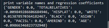
Predictor variables with regression coefficients equal to zero means that the coefficients for those variables had shrunk to zero after applying the LASSO regression penalty, and were subsequently removed from the model. So the results show that of the 9 variables, 3 were chosen in the final model. All the variables were standardized on the same scale so we can also use the size of the regression coefficients to tell us which predictors are the strongest predictors of drinking status. For example, White ethnicity had the largest regression coefficient and was most strongly associated with drinking status. Age and total number of relatives with drinking problems were negatively associated with drinking status.

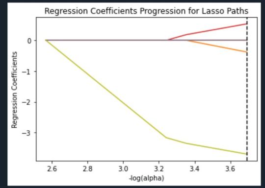
Regression Coefficients Progression Plot

This plot shows the relative importance of the predictor variable selected at any step of the selection process, how the regression coefficients changed with the addition of a new predictor at each step, and the steps at which each variable entered the new model. Age was entered first, it is the largest negative coefficient, then White ethnicity (the largest positive coefficient), and then Total Relatives (a negative coefficient).

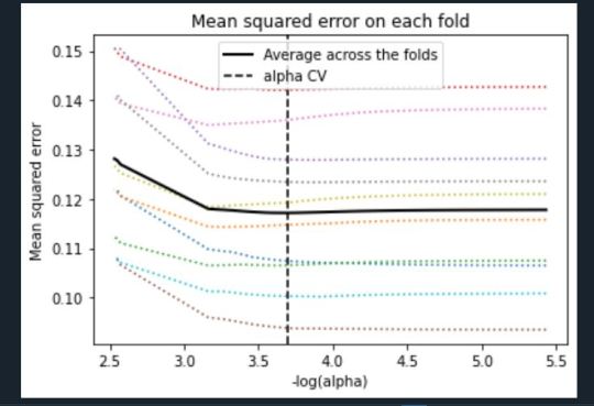
Mean Square Error Plot

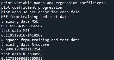
The Mean Square Error plot shows the change in mean square error for the change in the penalty parameter alpha at each step in the selection process. The plot shows that there is variability across the individual cross-validation folds in the training data set, but the change in the mean square error as variables are added to the model follows the same pattern for each fold. Initially it decreases, and then levels off to a point a which adding more predictors doesn’t lead to much reduction in the mean square error.

Mean Square Error for Training and Test Data

Training: 0.11656843533066587

Test: 0.11951981671418109

The test mean square error was very close to the training mean square error, suggesting that prediction accuracy was pretty stable across the two data sets.

R-Square from Training and Test Data

Training: 0.08961978111112545

Test: 0.12731098626365933

The R-Square values were 0.09 and 0.13, indicating that the selected model explained 9% and 13% of the variance in drinking status for the training and the test sets, respectively. This suggests that I should think about adding more explanatory variables but I must be careful and watch for an increase in variance and bias.

Python Code

os.environ['PATH'] = os.environ['PATH']+';'+os.environ['CONDA_PREFIX']+r"\Library\bin\graphviz"

data = pandas.read_csv('nesarc_pds.csv', low_memory=False)

## Machine learning week 3 addition## #upper-case all DataFrame column names data.columns = map(str.upper, data.columns) ## Machine learning week 3 addition##

#setting variables you will be working with to numeric data['IDNUM'] =pandas.to_numeric(data['IDNUM'], errors='coerce') data['AGE'] =pandas.to_numeric(data['AGE'], errors='coerce') data['SEX'] = pandas.to_numeric(data['SEX'], errors='coerce') data['S2AQ16A'] =pandas.to_numeric(data['S2AQ16A'], errors='coerce') data['S2BQ2D'] =pandas.to_numeric(data['S2BQ2D'], errors='coerce') data['S2DQ1'] =pandas.to_numeric(data['S2DQ1'], errors='coerce') data['S2DQ2'] =pandas.to_numeric(data['S2DQ2'], errors='coerce') data['S2DQ11'] =pandas.to_numeric(data['S2DQ11'], errors='coerce') data['S2DQ12'] =pandas.to_numeric(data['S2DQ12'], errors='coerce') data['S2DQ13A'] =pandas.to_numeric(data['S2DQ13A'], errors='coerce') data['S2DQ13B'] =pandas.to_numeric(data['S2DQ13B'], errors='coerce') data['S2DQ7C1'] =pandas.to_numeric(data['S2DQ7C1'], errors='coerce') data['S2DQ7C2'] =pandas.to_numeric(data['S2DQ7C2'], errors='coerce') data['S2DQ8C1'] =pandas.to_numeric(data['S2DQ8C1'], errors='coerce') data['S2DQ8C2'] =pandas.to_numeric(data['S2DQ8C2'], errors='coerce') data['S2DQ9C1'] =pandas.to_numeric(data['S2DQ9C1'], errors='coerce') data['S2DQ9C2'] =pandas.to_numeric(data['S2DQ9C2'], errors='coerce') data['S2DQ10C1'] =pandas.to_numeric(data['S2DQ10C1'], errors='coerce') data['S2DQ10C2'] =pandas.to_numeric(data['S2DQ10C2'], errors='coerce') data['S2BQ3A'] =pandas.to_numeric(data['S2BQ3A'], errors='coerce')

###### WEEK 4 ADDITIONS #####

#hispanic or latino data['S1Q1C'] =pandas.to_numeric(data['S1Q1C'], errors='coerce')

#american indian or alaskan native data['S1Q1D1'] =pandas.to_numeric(data['S1Q1D1'], errors='coerce')

#black or african american data['S1Q1D3'] =pandas.to_numeric(data['S1Q1D3'], errors='coerce')

#asian data['S1Q1D2'] =pandas.to_numeric(data['S1Q1D2'], errors='coerce')

#native hawaiian or pacific islander data['S1Q1D4'] =pandas.to_numeric(data['S1Q1D4'], errors='coerce')

#white data['S1Q1D5'] =pandas.to_numeric(data['S1Q1D5'], errors='coerce')

#consumer data['CONSUMER'] =pandas.to_numeric(data['CONSUMER'], errors='coerce')

data_clean = data.dropna()

data_clean.dtypes data_clean.describe()

sub1=data_clean[['IDNUM', 'AGE', 'SEX', 'S2AQ16A', 'S2BQ2D', 'S2BQ3A', 'S2DQ1', 'S2DQ2', 'S2DQ11', 'S2DQ12', 'S2DQ13A', 'S2DQ13B', 'S2DQ7C1', 'S2DQ7C2', 'S2DQ8C1', 'S2DQ8C2', 'S2DQ9C1', 'S2DQ9C2', 'S2DQ10C1', 'S2DQ10C2', 'S1Q1C', 'S1Q1D1', 'S1Q1D2', 'S1Q1D3', 'S1Q1D4', 'S1Q1D5', 'CONSUMER']]

sub2=sub1.copy()

#setting variables you will be working with to numeric cols = sub2.columns sub2[cols] = sub2[cols].apply(pandas.to_numeric, errors='coerce')

#subset data to people age 6 to 80 who have become alcohol dependent sub3=sub2[(sub2['S2AQ16A']>=5) & (sub2['S2AQ16A']<=83)]

#make a copy of my new subsetted data sub4 = sub3.copy()

#Explanatory Variables for Relatives #recode - nos set to zero recode1 = {1: 1, 2: 0, 3: 0}

sub4['DAD']=sub4['S2DQ1'].map(recode1) sub4['MOM']=sub4['S2DQ2'].map(recode1) sub4['PATGRANDDAD']=sub4['S2DQ11'].map(recode1) sub4['PATGRANDMOM']=sub4['S2DQ12'].map(recode1) sub4['MATGRANDDAD']=sub4['S2DQ13A'].map(recode1) sub4['MATGRANDMOM']=sub4['S2DQ13B'].map(recode1) sub4['PATBROTHER']=sub4['S2DQ7C2'].map(recode1) sub4['PATSISTER']=sub4['S2DQ8C2'].map(recode1) sub4['MATBROTHER']=sub4['S2DQ9C2'].map(recode1) sub4['MATSISTER']=sub4['S2DQ10C2'].map(recode1)

#### WEEK 4 ADDITIONS #### sub4['HISPLAT']=sub4['S1Q1C'].map(recode1) sub4['AMERIND']=sub4['S1Q1D1'].map(recode1) sub4['ASIAN']=sub4['S1Q1D2'].map(recode1) sub4['BLACK']=sub4['S1Q1D3'].map(recode1) sub4['PACISL']=sub4['S1Q1D4'].map(recode1) sub4['WHITE']=sub4['S1Q1D5'].map(recode1) sub4['DRINKSTAT']=sub4['CONSUMER'].map(recode1) sub4['GENDER']=sub4['SEX'].map(recode1) #### END WEEK 4 ADDITIONS ####

#Replacing unknowns with NAN sub4['DAD']=sub4['DAD'].replace(9, numpy.nan) sub4['MOM']=sub4['MOM'].replace(9, numpy.nan) sub4['PATGRANDDAD']=sub4['PATGRANDDAD'].replace(9, numpy.nan) sub4['PATGRANDMOM']=sub4['PATGRANDMOM'].replace(9, numpy.nan) sub4['MATGRANDDAD']=sub4['MATGRANDDAD'].replace(9, numpy.nan) sub4['MATGRANDMOM']=sub4['MATGRANDMOM'].replace(9, numpy.nan) sub4['PATBROTHER']=sub4['PATBROTHER'].replace(9, numpy.nan) sub4['PATSISTER']=sub4['PATSISTER'].replace(9, numpy.nan) sub4['MATBROTHER']=sub4['MATBROTHER'].replace(9, numpy.nan) sub4['MATSISTER']=sub4['MATSISTER'].replace(9, numpy.nan) sub4['S2DQ7C1']=sub4['S2DQ7C1'].replace(99, numpy.nan) sub4['S2DQ8C1']=sub4['S2DQ8C1'].replace(99, numpy.nan) sub4['S2DQ9C1']=sub4['S2DQ9C1'].replace(99, numpy.nan) sub4['S2DQ10C1']=sub4['S2DQ10C1'].replace(99, numpy.nan) sub4['S2AQ16A']=sub4['S2AQ16A'].replace(99, numpy.nan) sub4['S2BQ2D']=sub4['S2BQ2D'].replace(99, numpy.nan) sub4['S2BQ3A']=sub4['S2BQ3A'].replace(99, numpy.nan)

#add parents togetheR sub4['IFPARENTS'] = sub4['DAD'] + sub4['MOM']

#add grandparents together sub4['IFGRANDPARENTS'] = sub4['PATGRANDDAD'] + sub4['PATGRANDMOM'] + sub4['MATGRANDDAD'] + sub4['MATGRANDMOM']

#add IF aunts and uncles together sub4['IFUNCLEAUNT'] = sub4['PATBROTHER'] + sub4['PATSISTER'] + sub4['MATBROTHER'] + sub4['MATSISTER']

#add SUM uncle and aunts together sub4['SUMUNCLEAUNT'] = sub4['S2DQ7C1'] + sub4['S2DQ8C1'] + sub4['S2DQ9C1'] + sub4['S2DQ10C1']

#add relatives together sub4['SUMRELATIVES'] = sub4['IFPARENTS'] + sub4['IFGRANDPARENTS'] + sub4['SUMUNCLEAUNT']

def TOTALRELATIVES (row): if row['SUMRELATIVES'] == 0 : return 0 elif row['SUMRELATIVES'] >= 1 : return 1

sub4['TOTALRELATIVES'] = sub4.apply (lambda row: TOTALRELATIVES (row), axis=1)

sub4_clean = sub4.dropna()

sub4_clean.dtypes sub4_clean.describe()

###Machine Learning week 3 additions##

#select predictor variables and target variable as separate data sets

predvar = sub4_clean[['GENDER','TOTALRELATIVES', 'HISPLAT', 'WHITE', 'BLACK', 'ASIAN', 'PACISL', 'AMERIND', 'AGE']]

target = sub4_clean.DRINKSTAT

# standardize predictors to have mean=0 and sd=1 predictors=predvar.copy() from sklearn import preprocessing

predictors['GENDER']=preprocessing.scale(predictors['GENDER'].astype('float64')) predictors['TOTALRELATIVES']=preprocessing.scale(predictors['TOTALRELATIVES'].astype('float64')) predictors['HISPLAT']=preprocessing.scale(predictors['HISPLAT'].astype('float64')) predictors['WHITE']=preprocessing.scale(predictors['WHITE'].astype('float64')) predictors['BLACK']=preprocessing.scale(predictors['BLACK'].astype('float64')) predictors['ASIAN']=preprocessing.scale(predictors['ASIAN'].astype('float64')) predictors['PACISL']=preprocessing.scale(predictors['PACISL'].astype('float64')) predictors['AMERIND']=preprocessing.scale(predictors['AMERIND'].astype('float64')) predictors['AGE']=preprocessing.scale(predictors['AGE'].astype('float64'))

# split data into train and test sets pred_train, pred_test, tar_train, tar_test = train_test_split(predictors, target, test_size=.3, random_state=123)

# specify the lasso regression model model=LassoLarsCV(cv=10, precompute=False).fit(pred_train,tar_train)

# print variable names and regression coefficients print("print variable names and regression coefficients") coef_dict = dict(zip(predictors.columns, model.coef_)) print(coef_dict)

# plot coefficient progression print("plot coefficient progression") m_log_alphas = -numpy.log10(model.alphas_) ax = plt.gca() plt.plot(m_log_alphas, model.coef_path_.T) plt.axvline(-numpy.log10(model.alpha_), linestyle='--', color='k', label='alpha CV') plt.ylabel('Regression Coefficients') plt.xlabel('-log(alpha)') plt.title('Regression Coefficients Progression for Lasso Paths')

# plot mean square error for each fold print("plot mean square error for each fold") m_log_alphascv = -numpy.log10(model.cv_alphas_) plt.figure() plt.plot(m_log_alphascv, model.cv_mse_path_, ':') plt.plot(m_log_alphascv, model.cv_mse_path_.mean(axis=-1), 'k', label='Average across the folds', linewidth=2) plt.axvline(-numpy.log10(model.alpha_), linestyle='--', color='k', label='alpha CV') plt.legend() plt.xlabel('-log(alpha)') plt.ylabel('Mean squared error') plt.title('Mean squared error on each fold')

# MSE from training and test data print("MSE from training and test data") from sklearn.metrics import mean_squared_error train_error = mean_squared_error(tar_train, model.predict(pred_train)) test_error = mean_squared_error(tar_test, model.predict(pred_test)) print ('training data MSE') print(train_error) print ('test data MSE') print(test_error)

# R-square from training and test data print("R-square frpm training and test data") rsquared_train=model.score(pred_train,tar_train) rsquared_test=model.score(pred_test,tar_test) print ('training data R-square') print(rsquared_train) print ('test data R-square') print(rsquared_test)

1 note · View note

jdelatour · 9 years

Photo

I was in the mood for some Southern Style “Shrimp🍤 & Grits🍚 I added Roasted tomatoes🍅, Collard Greens🌿& White/yellow Cheddar cheese🍴😋 #HisPlate #HisChef #HomeCookedFood

#homecookedfood #hischef #hisplate #yummy food #food #breakfast #morning #brunch #summer

0 notes

amymarie23 · 4 years

Photo

Machine Learning Week 1: Classification Tree

Question for this part

Is Having Relatives with Drinking Problems associated with current drinking status?

Parameters

I kept the parameters for this question the same as all the other question. I limited this study to participants who started drinking more than sips or tastes of alcohol between the ages of 5 and 83.

Explanation of Variables

Response Variable: If the participant is currently drinking (Binary – Yes/No) –DRINKSTAT

· Currently Drinking – YES - 1

· Not Currently Drinking – No- 0 - I consolidated Ex-drinker and Lifetime Abstainer into a No category for the purposes of this experiment.

Explanatory Variables:

· TOTALRELATIVES: If the participant has relatives with drinking problems or alcohol dependence (Binary – Yes/No)

o If a participant has one or more relatives with drinking problems, they are consolidated into the Yes category.

· SEX – Male coded 1, Female coded 2

The Python Output

The python output shows the correct and incorrect classifications of our classification tree. The diagonal 0 and 734 represent the number of true negatives for drinking status, and the number of true positive for drinking status, respectively. The 0 on the bottom left represents the number of false negatives, classifying current drinkers as not regular drinkers. The 114 on the top right represents the number of false positives, classifying a non-current drinker as a current drinker. We can also look at the accuracy score, which is approximately 0.87, which suggests that the classification tree model has classified 87% of the sample correctly as either current drinkers or non-current drinkers.

Classification Tree

The Classification Tree shows DRINKSTAT, a binary drinking status response variable, as the target. If the participant has relatives with drinking problems or alcohol abuse and sex are the predictors, or explanatory variables.

The resulting tree starts with a split at X[1], the first explanatory variable, if the participant has relatives with drinking problems (here called TOTALRELATIVES). If the value for TOTALRELATIVES is less than 0.5, that is no relatives with drinking problems or alcohol abuse, since my binary variable has the value of zero equaling no relatives and one equaling one or more relatives. Then the observations move to the left side of the split and include 353 of 1,268 individuals in the training sample.

From this node, another split is made based on sex, variable X[0]. The split is made into male and female. Males were 1 and females were 2. There are 261 males with no relatives with drinking problems and 92 females with no relatives with drinking problems. Of those 261 males with no relatives with drinking problems or alcohol abuse, 34 are not current drinkers and 227 are current drinkers. Of the 92 females with no relatives with drinking problems or alcohol abuse, 8 are not current drinkers and 84 are current drinkers.

If we go back to the top of the tree and follow the right side to find X[1], there are 915 participants out of the 1,268 individuals in the training sample who have relatives with drinking problems or alcohol abuse. The next node is a split based on sex X[0]. There are 539 males with relatives with drinking problems or alcohol abuse and 376 females with relatives with drinking problems or alcohol abuse. Of those 539 males that have relatives with drinking problems or alcohol abuse, 103 are not current drinkers and 436 are current drinkers. Of the 376 females that have relatives with drinking problems or alcohol abuse, 68 are not current drinkers and 308 are current drinkers.

Summary

The results indicate that there are more current drinkers in the nodes for participants with relatives who have drinking problems or alcohol abuse.

Python Code

from pandas import Series, DataFrame import pandas import numpy import os import matplotlib.pylab as plt from sklearn.model_selection import train_test_split from sklearn.tree import DecisionTreeClassifier from sklearn.metrics import classification_report, confusion_matrix import sklearn.metrics

os.environ['PATH'] = os.environ['PATH']+';'+os.environ['CONDA_PREFIX']+r"\Library\bin\graphviz"

data = pandas.read_csv('nesarc_pds.csv', low_memory=False)

###### WEEK 4 ADDITIONS #####

#hispanic or latino data['S1Q1C'] =pandas.to_numeric(data['S1Q1C'], errors='coerce')

#american indian or alaskan native data['S1Q1D1'] =pandas.to_numeric(data['S1Q1D1'], errors='coerce')

#black or african american data['S1Q1D3'] =pandas.to_numeric(data['S1Q1D3'], errors='coerce')

#asian data['S1Q1D2'] =pandas.to_numeric(data['S1Q1D2'], errors='coerce')

#native hawaiian or pacific islander data['S1Q1D4'] =pandas.to_numeric(data['S1Q1D4'], errors='coerce')

#white data['S1Q1D5'] =pandas.to_numeric(data['S1Q1D5'], errors='coerce')

#consumer data['CONSUMER'] =pandas.to_numeric(data['CONSUMER'], errors='coerce')

data_clean = data.dropna()

data_clean.dtypes data_clean.describe()

sub1=data_clean[['IDNUM', 'AGE', 'SEX', 'S2AQ16A', 'S2BQ2D', 'S2BQ3A', 'S2DQ1', 'S2DQ2', 'S2DQ11', 'S2DQ12',

'S2DQ13A', 'S2DQ13B', 'S2DQ7C1', 'S2DQ7C2', 'S2DQ8C1', 'S2DQ8C2', 'S2DQ9C1', 'S2DQ9C2', 'S2DQ10C1', 'S2DQ10C2', 'S1Q1C', 'S1Q1D1', 'S1Q1D2', 'S1Q1D3', 'S1Q1D4', 'S1Q1D5', 'CONSUMER']]