#microsoft excel concatenate

[violetfractal]

Violet is playing Microsoft Excel...

You're listening to an ms excel fractal played one column at a time! Imagine the spreadsheet is sheet music with higher pitches toward the bottom. (The pitch for each row is in column C.)

I made this sound in miscrosoft excel! I made it in desmos. I used excel to generate excel formulas that generate desmos formulas that play music.

I was inspired by this arcade machine i saw.

wanna see some formula gore?

https://www.desmos.com/calculator/ecyjwrrg63

the desmos code is generated by excel:

A261="\operatorname{tone}("&C2&",L_{"&(ROW()-259)&"}[\operatorname{mod}(o,l_{"&(ROW()-259)&"})])"

B261="l_{"&(ROW()-259)&"}=\operatorname{length}(L_{"&(ROW()-259)&"})"

C261="L_{"&(ROW()-259)&"}=["&D261&"0]"

D261=CONCATENATE ???

you can't ask excel 2010 for concatenate(a1:a3). it will only take concatenate(a1,a2,a3). So I had to generate a list of cells to concatenate.

??? was generated recursively by:

E260=ADDRESS(ROW()+1,COLUMN(),4,1) F260=E260&","&ADDRESS(ROW()+1,COLUMN(),4,1)

[sunsetsspam]

I am so happy to be alive in a time where I can use the concatenate function on Microsoft excel

[fromdevcom]

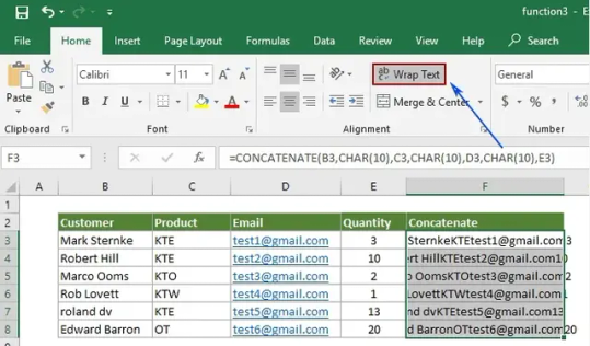
There are hundreds of built-in functions in Microsoft Excel. Furthermore, you can use these functions together in different combinations to create powerful formulas. The ability to create formulas in Excel that solve complex problems is largely what makes the application so legendary. With that in mind, we will now look at 10 Excel functions that you should add to your repertoire. IFERROR The IF function is probably one of the most widely used functions among Excel pros. It is a logical function; if something is true then do something, otherwise do something else. The ‘IF’ function allows you to build metadata - a set of data used to describe other data. Those same pros that use ‘IF’ also use the ‘IFERROR’ function to handle errors in their formulas. We can use ‘IFERROR’ to specify an alternative value where a calculation might result in an error. Let’s look at the ‘IFERROR’ function’s syntax:                       =IFERROR(value, value-if-error) There are two arguments in this formula: ‘value’ and ‘value-if-error’. The ‘value’ argument is the parameter the function tests for an error. This is most often another formula itself. Then the ‘value-if-error’ argument is the replacement value the user has selected for ‘IFERROR’ to return if the ‘value’ parameter does result in an effort. The ‘value-if-error’ can be an actual static value such as a string or a number, but it can also itself be another formula. In the example that follows, we have an average price calculation in the ‘Average Price’ column. It is a simple division calculation that is susceptible to a divide by zero error (#DIV/0!). In cell D6, this is precisely what has happened. However, by using the ‘IFERROR’ function, we can ensure that the value ‘0’ gets returned to the cell in the case of an error. Note the improvement to our result for row 6 in cell E6. COUNTIF Another popular ‘IF’ based function is ‘COUNTIF’. This function counts cells in a range where some specified condition is met. The syntax is simple. There are two arguments: ‘range’ and ‘criteria’. The ‘range’ argument is the range in which you are searching for the ‘criteria’. The ‘criteria’ argument is the specific condition that needs to be met for the count                                  =COUNTIF(range, criteria) In the following example, we use ‘COUNTIF’ to count the number of employees by their years of service. Our ‘range’ argument is the column containing the ‘Year of Service’ for each employee, or “D2: D19” (the dollar signs preceding the column and row references are simply there to ‘lock’ the range for dragging the formula to other cells). The ‘criteria’ argument is the years of service (1, 2 or 3). We could have placed the literal number values for ‘Years of Service’ as our ‘criteria’, but in this case, we opted to use the cell references for each (“F3”, “F4”, and “F5”, respectively). The ‘COUNTIF’ formula in each returns the count of employees corresponding to each value in ‘Years of Service’ in column G. Note the formulas for each row in column H. CONCATENATE The ‘CONCATENATE’ function is one of the most widely used in Excel. A point worth noting is that Microsoft introduced two new functions in Excel 2016 that will eventually replace ‘CONCATENATE’. They are ‘CONCAT’, a more flexible version of its predecessor, and ‘TEXTJOIN’. However, since not all Excel users have upgraded to Excel 2016, we will look at ‘CONCATENATE’. The ‘CONCATENATE’ function combines strings of text and/or numerical values. Syntactically, this simply means placing the values you want to concatenate in sequential order, separated by commas. You can use either literal values or cell references as your arguments. You can use a combination of both as well.                                         =CONCATENATE(text1,[text2],…) In the following example, we have two separate lists: first names and last names. Using the ‘CONCATENATE’ function, we will combine them in a column where we have the last name, then the first name separated by a comma.

Then we can sort each by the last name in alphabetical order. VLOOKUP If you have spent much time with anyone with a reasonable amount of proficiency using Excel, you have likely heard of ‘VLOOKUP’. Like its sibling, ‘HLOOKUP’, it will search a table of values based on a criteria value. The ‘VLOOKUP’ function will search the first column of a table for a criteria value and return a value from some specified number of columns to the right of that first column. The function consists of four arguments.                  =VLOOKUP(lookup_value, table_array, col_index_number, [range_lookup]) The first argument is the ‘lookup_value’ is the value ‘VLOOKUP’ seeks a match for in the ‘table_array’ argument. In the following example, this is the cell reference ‘E2’ where we see the string ‘Finance’. We could have just as easily used the literal string ‘Finance’ as our ‘lookup_value’ argument. But using the cell reference allows us to change the value in ‘E2’ without changing the formula. The ‘table_array’ is the table of values ‘VLOOKUP’ will seek a match for ‘Finance’ in the first column. Since our table is ‘A2: C7’, the match for our ‘lookup_value’ is on the first row (cell ‘A2’) of our ‘table_array’, The ‘col_index_number’ argument is the number of the column from which we want ‘VLOOKUP’ to return a match on the same row from the ‘lookup_value’. In our case, we want ‘Average Years of Service’ in our formula in cell ‘F2’. This means we will insert ‘2’ as our ‘col_index_number’ argument since ‘Average Years of Service’ is the second column in our ‘table_array’. The ‘range_lookup’ argument is an optional argument as denoted by the square brackets. This argument can be one of two values: TRUE or FALSE. A TRUE value tells the ‘VLOOKUP’ to return an approximate match while a FALSE value tells it to return an exact match. When omitted, the default for the formula is an approximate match. In the following example, we can easily look up the average years of service and the average salary for employees by specifying the department. An insider trick regarding ‘range_lookup’: try using ‘1’ and ‘0’ as a substitute for TRUE and FALSE, respectively. This is a shortcut that works just the same. Note in ‘G2’ our ‘VLOOKUP’ uses ‘0’ instead of FALSE. INDEX And MATCH The combination of ‘INDEX’ and ‘MATCH’ function gives users the ability to retrieve data from a table by specifying the row and column condition. Combining the two in a single formula creates one of the most well-known lookup formulas used. The most basic example of what the ‘INDEX’ function does is that it takes an array, like a column of names. Then it takes a second argument, ‘row_num’, and returns the value from the array on that row.                                       =INDEX(array, row_num, [column_num]) Note that since we are working with a single column, we omit the optional ‘column_num’ argument since it is implied. However, if we were working with an array that had more than one column, we would use the ‘column_num’ argument in the same way we use the ‘row_num’ argument. ‘INDEX’ will return the value at the intersection of the two in the specified ‘array’. In the following example, the ‘column_num’ is understood to be 1. This means the formula finds the value at the intersection of row 6 and column 1 of our ‘array’, ‘A2: A19’. The ‘MATCH’ function takes a ‘lookup_value’, a ‘lookup_array’, and an optional ‘match_type’ argument. The ‘match_type’ argument allows for one of three values; ‘-1’ for less than, ‘0’ for an exact match, or ‘1’ for greater than.                      =MATCH(lookup_value, lookup_array, [match_type]) In the next example, we pass in a string value for the ‘lookup_value’ and ‘0’ to ‘match_type’ for an exact match. See cell ‘C12’ for the result. Now you have seen how you can find the row on which a value exists in a column using the ‘MATCH’ function. You have also seen how you can find the value in a cell by passing in a row number to the ‘INDEX’ function.

Imagine you had a second column with email addresses that you wanted to look up by employee name. See if you can figure out how to combine ‘INDEX’ with ‘MATCH’ to do just that. Hint: substitute the ‘MATCH’ formula for the ‘row_num’ argument in the ‘INDEX’ formula – then make sure you select the email column as the ‘array’ for your ‘INDEX’ function. GETPIVOTDATA If you have ever tried referring to a cell or range in a Pivot Table, you have probably seen ‘GETPIVOTDATA’. The GETPIVOTDATA function helps retrieve data from a pivot table using the corresponding row and column value. This function is yet another type of lookup function but for Pivot Table users. It provides a direct method of retrieving tabulated data from Pivot Tables.                  =GETPIVOTDATA(data_field ,pivot_table, [field1, item1], …) The first argument, ‘data_field’, refers to the data field from which we want our result. In the following example, this will be our Pivot Table columns. The second argument, ‘pivot_table’, refers to the actual Pivot Table. In the following example, this is simply the cell reference ‘I3’, which is cell where our Pivot Table originates. The third and fourth arguments, ‘field1’ and ‘item1’, refer to the field and row on which we want a match in the ‘data_field’. In our example below, our first ‘GETPIVOTDATA’ formula is looking for a match to the finance department in the ‘Average of Years of Service’ column. Note that instead of hard-coding the literal value ‘Finance’ for the ‘item1’ argument, we have used the cell reference ‘N4’ where we have entered that string value. Just as we have seen with the other formulas we have covered, literal values or cell references can be used. TEXTJOIN We alluded to one of the newest functions in Excel, ‘TEXTJOIN’, in our earlier discussion about ‘CONCATENATE’. This function is only available in Excel 2016 desktop or in Excel online as a part of Microsoft 365. Recall that the ‘CONCATENATE’ function requires an individual cell reference for each string. However, the ‘TEXTJOIN’ function allows you to combine strings by referring to multiple cells in a range. Usage of the ‘TEXTJOIN’ function is simple. There are three arguments.                                    =TEXTJOIN(delimiter, ignore_empty, text1, …) The first argument, ‘delimiter’, is any string you want to be placed between the joined elements. This could be a symbol like a comma(“,”), or it could be a space (“ “). If you want nothing between the string elements you are joining, you still must specify that with the ‘delimiter’ argument. You simply insert two double quotes with nothing in between (“”). The second argument, ‘ignore_empty’, allows you to tell the function whether you want to skip over empty cells when joining their values. This is simply a TRUE value for ignoring blanks, or FALSE when you do not want to ignore blanks. The ‘text1’ argument is simply the cell or range of values you want to join. One thing to note is that you can add multiple ‘text’ arguments for each cell or range you want to be a part of the ‘TEXTJOIN’ formula. Notice that we have a few blank cells in our range “A2: A19” but since we chose TRUE for the ‘ignore_empty’ argument, our result in the merged range “C2: G10” indicates no missing values between any of the commas. FORMULATEXT The ‘FORMULATEXT’ function returns the formula for a specific cell reference. If a formula is not present, the error value ‘#N/A’ results. This function provides an alternative way to visualize the formula present in a cell. The syntax is incredibly simple:                                           =FORMULATEXT(reference) The single argument, ‘reference’, is the cell reference where the formula exists. In the following example, there are multiplication formulas in column C. Placing a ‘FORMULATEXT’ function in the D column that references the cells on the same row in C, we can now visualize the formula as well as the result. IFS Another of the new functions available with Excel 2016 and Excel Online is the ‘IFS’ function.

This function works in similar fashion as the ‘IF’ function, but it goes further by providing an efficient method of incorporating multiple logical tests and multiple values. Where in the past the same results would require nested ‘IF’ functions, the ‘IFS’ simplifies this process.                                              =IFS(logical_test1, value_if_true1, ...) In this example, we can assign a description of performance without utilizing nested IF statements. Download Sample File  With the hundreds of available built-in functions with which to build your own formulas with, this list is by no means comprehensive. Furthermore, some of the functions on this list may not even resonate with your needs. However, we curated the list with broad appeal in mind and feel that most Excel users could find a way to leverage these at some point. Sometimes the simplest functions lead to formulas that create great value. Moreover, sometimes it is difficult to know what is possible until you see them in action. We hope you find this list helpful and inspiring! 

[tccicomputercoaching]

Advanced Excel Formulas You Must Know Today

Introduction

Microsoft Excel is vital for data analysis, financial modeling, and business decision-making. While basic formulas are useful, Advanced Excel Formulas You Must Know Today can significantly boost productivity. This blog highlights essential advanced Excel formulas to help you work smarter and more efficiently.

Why Advanced Excel Formulas Matter?

Grasping the advanced formulas will help you:

Automate repetitive tasks

Enhance the accuracy of data analysis

Efficiently deal with large datasets

Save time and improve productivity

Above all, advanced Excel formulas will boost your effectiveness in Excel regardless of whether you are an analyst, an accountant, or a student.

Top Advanced Excel Formulas You Must Learn

1. INDEX-MATCH (Powerful Alternative to VLOOKUP)

Formula: =INDEX(range, MATCH(lookup_value, lookup_range, match_type))

INDEX-MATCH is a powerful combination that replaces VLOOKUP for better accuracy and flexibility.

2. VLOOKUP and HLOOKUP

Formula: =VLOOKUP(lookup_value, table_array, col_index_num, [range_lookup])

VLOOKUP is commonly used for looking up values in vertical columns, whereas HLOOKUP does the same for horizontal rows.

3. XLOOKUP (New Alternative to VLOOKUP)

Formula: =XLOOKUP(lookup_value, lookup_array, return_array, [if_not_found], [match_mode], [search_mode])

XLOOKUP simplifies searches with more flexibility and fewer limitations than VLOOKUP.

4. IF, AND, OR (Logical Functions)

Formula: =IF(condition, value_if_true, value_if_false)

Logical functions like IF, AND, and OR help in decision-making processes within Excel.

5. SUMIFS and COUNTIFS (Conditional Calculations)

Formula: =SUMIFS(sum_range, criteria_range1, criteria1, [criteria_range2, criteria2, ...])

SUMIFS and COUNTIFS allow users to sum or count values based on multiple criteria.

6. TEXT and CONCATENATE (String Functions)

Formula: =TEXT(value, format_text)

These functions help in formatting numbers and combining text efficiently.

7. OFFSET and INDIRECT (Dynamic Ranges)

Formula: =OFFSET(reference, rows, cols, [height], [width])

OFFSET and INDIRECT are useful for working with dynamic ranges and references.

8. CHOOSE (Multiple Conditions Handling)

Formula: =CHOOSE(index, value1, value2, value3, …)

This function helps select a value from a list based on an index number.

9. UNIQUE and FILTER (Dynamic Array Functions)

Formula: =UNIQUE(array)

These functions help filter unique values and retrieve filtered data dynamically.

10. LET and LAMBDA (New Functions for Efficiency)

Formula: =LET(name, value, calculation)

LET and LAMBDA simplify formulas by allowing users to define variables within Excel formulas.

Optimizing productivity with advanced formulas

Calculations are thus automated and errors minimized

Manual processes are thus eliminated, saving time

Faster and improved are data analysis and reporting

Advanced Excel formulas in practice

Financial modeling using VLOOKUP and SUMIFS

Data Analysts have two advanced functions: INDEX-MATCH and FILTER

Business Reporter with UNIQUE and TEXT functions

Common mistakes when performing formulas

Incorrectly selecting ranges

Not using absolute references ($A$1) when called for

Forgetting about dynamic ranges

How to learn advanced Excel at TCCI-Tririd Computer Coaching Institute

Advanced Excel programs are taught at TCCI-Tririd Computer Coaching Institute by tutors expert in their fields. A practical-oriented training ensures students can practically use Excel capabilities.

Conclusion

Mastering advanced formulas on Excel can greatly help your efficiency and data management. Whether you are starting out or have some experience, gaining such formulas will propel you on the way to advanced Excel skills.

Location: Bopal & Iskon-Ambli Ahmedabad, Gujarat

Call now on +91 9825618292

Get information from: tccicomputercoaching.wordpress.com

FAQs

1. What is the strongest Excel formula?

The INDEX-MATCH combination is regarded as one of the strongest Excel formulas for performing efficient data lookup.

2. Is learning Advanced Excel hard?

Not at all! With adequate guidance and practice, anyone can learn Advanced Excel at TCCI-Tririd Computer Coaching Institute.

3. Is VLOOKUP or XLOOKUP better?

XLOOKUP is more powerful as it overcomes many limitations of VLOOKUP, such as leftward searches.

4. Will I be able to automate reports using Excel formulas?

Yes! Formulas like SUMIFS, INDEX-MATCH, and UNIQUE help automate data processing and reporting.

5. Where do I learn Advanced Excel in Ahmedabad?

You can register for expert training on Advanced Excel at TCCI-Tririd Computer Coaching Institute.

[advancedexcelinstitute]

The Best Advanced Excel Corporate Trainers in Delhi: What to Expect

When it comes to mastering Advanced Excel and VBA Macros, Advanced Excel Institute, stands out as a leader in corporate training. Led by Pankaj Kumar Gupta, a Microsoft Certified Trainer with over a decade of experience, the institute has built a reputation for delivering impactful training that equips employees with practical, high-level Excel skills. Here’s what to expect from training sessions with Pankaj Sir, Advanced Excel Corporate Trainer.

1. Expert Trainer with a Proven Track Record

He has conducted over 500 corporate training sessions, training more than 10,000 professionals across various industries. His extensive experience and Microsoft certification make him one of the most trusted Advanced Excel and VBA Macros trainers in Delhi. Known for his practical teaching style, focuses on real-world applications, ensuring that employees can immediately apply what they learn.

2. Customized Training Approach

They understands that each organization has unique needs. The training sessions are design in tailored to the specific requirements of each company, whether it's for data analysis, reporting, automation, or financial modeling. This tailored approach ensures that the training content matches the company's objectives and supports the employees' daily responsibilities.

3. Hands-On, Practical Learning

Further, his sessions are highly interactive and focus on practical learning. Rather than just theory, his training includes real-time database examples and hands-on exercises. Employees learn to work with advanced functions like VLOOKUP, HLOOKUP, INDEX/MATCH, and SUMIFS. They also explore Pivot Tables, data visualization, and chart creation to handle complex data sets effectively.

4. Advanced Excel and VBA Macros Expertise

As an expert in both Advanced Excel and VBA Macros, He covers a wide range of topics that boost efficiency and accuracy in data management. His VBA Macros training is particularly valuable for automating repetitive tasks, saving time, and minimizing errors. This enables employees to increase productivity significantly, making them more valuable assets to the organization.

5. Comprehensive Curriculum

Training sessions at Advanced Excel Institute are structured to cover essential and advanced topics, including:

Formulas and Functions: Covering basic to advanced functions like IF, SUMPRODUCT, CONCATENATE, and logical functions.

Data Management: Techniques for managing data across multiple sheets, using features like Advanced Filter, Data Validation, and Text to Columns.

Data Analysis and Visualization: Creating Pivot Tables, Pivot Charts, and various types of charts (e.g., Gantt charts, Bubble charts) to make data analysis easier and more insightful.

VBA Macros: Automating workflows, writing simple to complex Macros, and using VBA to streamline daily tasks.

6. Focus on Productivity and Efficiency

One of the main goals of the training is to help employees work faster and smarter. He teaches productivity-boosting techniques, including Excel shortcuts, effective use of the Name Manager, and advanced filtering options. These tools and tricks enable employees to complete their tasks in less time with higher accuracy.

7. Post-Training Support and Resources

After the training, Pankaj and Advanced Excel Institute provide post-training support to help employees resolve any doubts and reinforce what they’ve learned. This ongoing support ensures that employees are confident and fully equipped to apply their skills in real-world scenarios.

8. Strong Industry Reputation

With experience conducting training in major Indian cities like Delhi, Gurgaon, Mumbai, Bangalore, and Hyderabad, Advanced Excel Institute has built a strong reputation nationwide. Numerous companies trust them to deliver effective training that enhances employees’ skills in Advanced Excel and VBA Macros.

Choosing Pankaj Kumar Gupta as an Excel Corporate Trainer in Delhi for corporate training ensures that your team will receive practical, high-quality instruction that directly impacts productivity and accuracy in data management. With a focus on hands-on learning, real-world applications, and post-training support, Advanced Excel Institute stands out as one of the best training providers in Delhi for Advanced Excel and VBA Macros.

 For more information, contact us at:

Call: 8750676576, 871076576

Email:advancedexcel07@gmail.com

Website:www.advancedexcel.net

[esscomputerinstitute]

Top 10 Excel Tricks You Should Know

Excel is a versatile tool widely used for data management, analysis, and visualisation. As part of the Microsoft Office suite, Excel is indispensable for students and professionals, offering a platform to organise and process information efficiently. Its ability to perform calculations, create charts, and handle large datasets makes it an essential skill in academics, business, and everyday problem-solving. If you want to enhance your skills, learning these 10 tricks will make your work easier and more efficient.

1. Use Pivot Tables to Summarise Data

Pivot Tables help you quickly summarise large datasets. Instead of manually calculating totals or averages, you can use this tool to analyse your data with a few clicks. For example, if you have sales data for different regions, a Pivot Table can display total sales by region in seconds. Mastering Pivot Tables can give you an edge in any Excel course, as this feature is highly valued in data analysis.

2. Split Data into Separate Columns

When you have combined data, like full names or addresses, in one column, you can split it into multiple columns using the “Text to Columns” feature. Go to the “Data” tab, click “Text to Columns,” and choose how you want to split the data, such as by space or comma. This trick is especially useful for cleaning datasets before working on projects or assignments.

3. Transpose Rows and Columns

Need to switch rows into columns or vice versa? The transpose feature saves time and effort. Copy your data, right-click where you want to paste it and select “Transpose.” This simple trick is handy for reorganising data layouts.

4. Apply Conditional Formatting

Conditional Formatting highlights cells based on specific criteria. For instance, you can make all cells with marks above 90 turn green. Select your data, go to “Home” > “Conditional Formatting,” and set your rules. This trick helps you visually track trends or patterns in your data.

5. Remove Duplicate Data

Removing duplicates makes sure that your data is accurate and free from redundancy. Highlight the relevant column, go to the “Data” tab, and click “Remove Duplicates.” This trick is essential for students dealing with multiple datasets, such as when merging survey results or reports.

6. Use the IF Formula for Logical Conditions

The IF formula allows you to create logical conditions. For example, you can use it to check if marks are above a certain threshold and assign a grade accordingly. The formula format is =IF(condition, value_if_true, value_if_false). Learning this formula in an advance Excel course will help you automate repetitive tasks.

7. Leverage VLOOKUP to Find Data

VLOOKUP (Vertical Lookup) is useful when you need to search for data in a table. For example, if you have a list of student IDs and want to match them with their names, VLOOKUP can retrieve the relevant information instantly. It is an invaluable tool for assignments that involve cross-referencing data.

8. Use Filters to Simplify Data

Filters allow you to display only the rows you need. Click on the “Data” tab, select “Filter,” and use the dropdown options in each column to sort or filter your data. Filters are perfect for students working with large datasets, enabling them to focus on specific categories, such as filtering out overdue tasks.

9. Combine Text with the CONCATENATE Function

The CONCATENATE function merges text from multiple cells into one. For instance, if you have separate columns for first and last names, you can combine them into a full name using =CONCATENATE(A1, “ “, B1). This trick is particularly useful for creating clean, professional datasets.

10. Lock Cells with Absolute References

You might want specific cell references to remain constant when working with formulas, even when the formula is copied. Adding a dollar sign ($) before the column and row (e.g., $A$1) locks the reference. This trick prevents calculation errors, making it a fundamental concept covered in any Excel course.

Why Should You Learn These Tricks?

Mastering these Excel tricks will help you work smarter, not harder. These skills are invaluable for students in any field, from managing complex datasets to automating repetitive tasks. By enrolling in an advance Excel institute like ESS Institute, you can gain practical experience and build expertise in advanced features that will make your assignments and projects stand out. These tips are just the beginning. If you want to become proficient and gain an edge in academics or your career, it is time to invest in learning Excel.

Explore an advance Excel course at ESS Institute to unlock the full potential of this powerful tool!

[virtualemployeeblog]

Top 5 Excel Functions Every Expert Should Master 

Mastery of any data analysis tool like Excel comes with an addition to productivity and efficiency that is very significant. You can hire Microsoft excel experts who are experts in these functions: 

VLOOKUP- This function finds an item in a table or range and returns the corresponding value in another column. It is very helpful for the process of data lookup as well as matching. 

SUMIF - Sum cells in range that meet certain conditions. It is very commonly applied for filtering, aggregation, or calculation of data; for instance, it will sum up the sales within a specific type of product. 

COUNTIF - Like SUMIF, it counts the number of cells within a given range that meets criteria. It is helpful in running data analysis and also in reporting. 

IF - This function is designed to produce a logical test. Once this test becomes true, then it will yield some values; else it will yield different values. It plays a crucial role in formulating conditional formulas and making decisions. 

CONCATENATE - This function takes one or more text strings and returns them as a single text string. It's extremely useful when creating custom labels, reports, or indeed any other type of text-based output. Using CONCATENATE, you can take separate columns for first and last names and create one single name column with them. 

Anyone who is preparing for excel programmers for hire purposes must know these functions to tackle different types of data analysis jobs in the competitive landscape. 

[ajguides]

Excel - Split text into different columns with the Convert Text to Columns Wizard

Excel - Split text into different columns with the Convert Text to Columns Wizard | https://tinyurl.com/2b5oot8v | #Guide #Microsoft If you exporting data into CSV or text files then this guide may come in handy for you… You can take the text in one or more cells, and spread it out across multiple cells. This is called parsing, and is the opposite of concatenating, where you can combine text from two or more cells into one cell. For example, if you have a column of full names, you can split that column into separate first name and last name columns, like this: Go to Data > Text to Columns, and the wizard will walk you through the process. Here’s […] Read more... https://tinyurl.com/2b5oot8v

[korshubudemycoursesblog]

Unlocking the Full Potential of Microsoft Excel - From Beginner to Expert

In today's data-driven world, Microsoft Excel has become an indispensable tool for professionals across various industries. Whether you're a novice or someone looking to hone your skills, mastering Excel can significantly enhance your productivity and career prospects. This comprehensive guide, "Microsoft Excel - Beginner to Expert," will take you through everything you need to know to become an Excel pro. As we promote Udemy courses at Korshub, we recommend exploring online courses to supplement your learning journey.

Why Learn Microsoft Excel?

Microsoft Excel is more than just a spreadsheet program; it's a powerful tool that can help you analyze data, create complex reports, and make data-driven decisions. Excel skills are highly valued in the job market, and they can open doors to a wide range of career opportunities. Whether you're in finance, marketing, or any other field, Excel proficiency is a must-have skill.

Key Benefits of Learning Microsoft Excel:

Data Analysis: Excel allows you to analyze large datasets efficiently, helping you make informed decisions.

Automation: With features like macros and formulas, Excel can automate repetitive tasks, saving you time and effort.

Visualization: Create stunning charts and graphs to present your data clearly and concisely.

Versatility: Excel can be used for budgeting, project management, inventory tracking, and more.

Getting Started with Microsoft Excel - Beginner to Expert

1. Understanding the Excel Interface

Before diving into the more advanced features, it's essential to familiarize yourself with the Excel interface. The Ribbon, Quick Access Toolbar, and Workbook are some of the key components you'll interact with regularly.

The Ribbon: This is the top part of the Excel window that contains tabs like Home, Insert, Page Layout, and more. Each tab has a group of related commands.

Quick Access Toolbar: Located above the Ribbon, this toolbar provides easy access to commonly used commands.

Workbook: A workbook is the file in which you work, and it can contain one or more Worksheets.

2. Basic Excel Functions

Once you're comfortable with the interface, it's time to learn some basic Excel functions. These functions will form the foundation of your Excel skills.

SUM: Adds up all the numbers in a range of cells.

AVERAGE: Calculates the average of a range of numbers.

COUNT: Counts the number of cells that contain numbers.

MIN/MAX: Finds the minimum and maximum values in a range.

IF: Performs a logical test and returns one value if true and another if false.

Advanced Excel Skills

As you progress from beginner to expert, you'll need to master more advanced Excel skills. These skills will allow you to handle complex tasks and make the most out of Excel's powerful features.

3. Excel Formulas and Functions

Excel has hundreds of built-in formulas and functions that can perform calculations, manipulate data, and more. Some of the most commonly used advanced functions include:

VLOOKUP/HLOOKUP: Searches for a value in a table and returns a corresponding value in the same row or column.

INDEX/MATCH: A more flexible alternative to VLOOKUP, allowing you to search for a value in any row or column.

TEXT: Converts numbers to text, formats numbers, and more.

CONCATENATE: Joins two or more text strings into one.

4. Data Visualization with Excel

Creating charts and graphs is one of the most effective ways to visualize your data. Excel offers a variety of chart types, including Bar Charts, Pie Charts, Line Charts, and more.

Pivot Tables: A powerful tool for summarizing large datasets. Pivot Tables allow you to group, filter, and analyze data in a way that's easy to understand.

Conditional Formatting: This feature allows you to apply formatting based on specific conditions, making it easier to identify trends and outliers in your data.

Mastering Excel for Business

In a business context, Excel is invaluable for tasks like budgeting, forecasting, and reporting. Here are some advanced techniques that are particularly useful in a business setting.

5. Financial Modeling

Excel is widely used in finance for building financial models. These models can be used for budgeting, forecasting, and valuation purposes.

Discounted Cash Flow (DCF) Analysis: A method of valuing a company or project based on its expected future cash flows.

Scenario Analysis: Allows you to evaluate the impact of different variables on your financial model.

6. Excel Macros and VBA

For those who want to take their Excel skills to the next level, learning Macros and Visual Basic for Applications (VBA) is essential. Macros allow you to automate repetitive tasks, while VBA enables you to create custom functions and automate complex processes.

Top Tips for Becoming an Excel Expert

7. Practice, Practice, Practice

The key to mastering Excel is consistent practice. The more you use Excel, the more comfortable you'll become with its features and functions.

8. Leverage Online Resources

There are countless online resources available to help you learn Excel. At Korshub, we recommend checking out Udemy courses for in-depth tutorials and practical exercises.

Excel forums: Online communities where you can ask questions and share tips with other Excel users.

YouTube tutorials: A great way to learn new Excel techniques and tricks.

Blogs and articles: Stay updated with the latest Excel trends and features by following Excel-related blogs.

9. Stay Updated with Excel Updates

Microsoft regularly updates Excel with new features and improvements. Make sure to keep your Excel version up-to-date to take advantage of these enhancements.

Common Mistakes to Avoid in Excel

Even experienced Excel users can make mistakes. Here are some common pitfalls to watch out for:

Not backing up your work: Always save your work regularly to avoid losing important data.

Incorrect use of formulas: Double-check your formulas to ensure they are working as expected.

Not using shortcuts: Excel has many keyboard shortcuts that can save you time. Learn and use them regularly.

Overcomplicating your spreadsheet: Keep your spreadsheet simple and organized to avoid confusion and errors.

Conclusion

Mastering Microsoft Excel - Beginner to Expert is a journey that requires time, patience, and practice. However, the benefits of becoming proficient in Excel are well worth the effort. Whether you're looking to advance your career, increase your productivity, or simply manage your personal finances more effectively, Excel is an invaluable tool.

At Korshub, we promote Udemy courses that can help you achieve your Excel mastery goals. Explore our recommended courses and start your journey from beginner to expert today. Remember, the key to success in Excel is continuous learning and practice. So, keep exploring, experimenting, and pushing the boundaries of what's possible with Excel.

[hob28]

Microsoft Excel Advanced Course - Elevate Your Excel Mastery

Microsoft Excel is a cornerstone of productivity in the business world. From data analysis to financial modeling, Excel’s capabilities are vast. However, to truly leverage its potential, you need advanced knowledge beyond the basics. Whether you’re a professional looking to improve efficiency or a student aiming to gain an edge, enrolling in a Microsoft Excel Advanced Course can significantly enhance your skillset. This article explores the benefits of such a course, what it covers, and how it can propel your career forward.

Why an Advanced Excel Course is a Must-Have

While many people are familiar with Excel’s basic functions, few fully grasp its advanced features. Mastering these can drastically improve your work efficiency and the quality of your output. Here’s why you should consider taking a Microsoft Excel Advanced Course:

Enhanced Data Management: Learn how to manage and analyze large datasets with advanced functions like PivotTables, Power Query, and data modeling.

Increased Efficiency: Automate repetitive tasks using macros and VBA, saving time and reducing errors.

Better Decision-Making: Use advanced data analysis tools to derive insights and make informed business decisions.

Career Advancement: Excel proficiency is highly valued by employers, making it a critical skill for career growth.

By upgrading your Excel skills, you position yourself as a more competent and valuable professional in any industry.

What You’ll Learn in a Microsoft Excel Advanced Course

A Microsoft Excel Advanced Course is designed to equip you with expert-level skills that can be applied across various professional scenarios. Here’s an overview of the core topics typically covered:

1. Advanced Formulas and Functions

Complex Formulas: Learn to create and troubleshoot complex formulas involving multiple functions.

Logical Functions: Master functions like IF, AND, OR, and XOR to create dynamic spreadsheets.

Text Functions: Manipulate text data with functions like LEFT, RIGHT, MID, and CONCATENATE.

2. Data Analysis Techniques

PivotTables: Deep dive into PivotTables to summarize, filter, and analyze large datasets.

Power Query: Automate data import, cleaning, and transformation tasks with Power Query.

What-If Analysis: Use tools like Goal Seek, Solver, and Data Tables to evaluate different business scenarios.

3. Macros and VBA Programming

Macro Recording: Record macros to automate routine tasks with a single click.

Introduction to VBA: Learn the basics of Visual Basic for Applications (VBA) to write custom scripts for Excel.

Custom Functions: Create your own Excel functions using VBA to solve specific problems efficiently.

4. Data Visualization

Advanced Charts: Create sophisticated charts like histograms, Gantt charts, and Pareto charts.

Conditional Formatting: Use advanced conditional formatting to highlight key data trends and outliers.

Dashboards: Design interactive dashboards that consolidate key metrics and make data-driven insights easily accessible.

5. Data Validation and Security

Data Validation: Set up rules to ensure the integrity and accuracy of data entry.

Workbook Protection: Learn how to protect sensitive data using Excel’s built-in security features.

Collaboration Tools: Manage and track changes in shared workbooks effectively.

Who Should Enroll in a Microsoft Excel Advanced Course?

This course is ideal for anyone who regularly works with data, including:

Business Analysts: Improve your ability to analyze complex datasets and present findings.

Financial Professionals: Enhance your financial modeling skills and automate processes.

Project Managers: Track project data, budgets, and timelines more efficiently.

Entrepreneurs: Gain the skills to manage and analyze business data for better decision-making.

An advanced Excel course can make a significant impact on your productivity and career trajectory, no matter your field.

Benefits of a Microsoft Excel Advanced Course

Here’s why investing in an advanced Excel course is worthwhile:

Boosted Efficiency: Automate tasks, streamline workflows, and save valuable time.

Improved Data Accuracy: Learn to manage data more effectively, reducing errors and inconsistencies.

Career Growth: Excel proficiency is a marketable skill that can lead to promotions and higher-paying roles.

Certification: Upon completion, many courses offer certification, validating your expertise and enhancing your resume.

How to Choose the Right Microsoft Excel Advanced Course

When selecting a course, consider the following:

Course Curriculum: Ensure the course covers advanced topics relevant to your work or interests.

Instructor Qualifications: Opt for courses taught by industry experts with real-world experience.

Learning Format: Decide between online or in-person classes based on your learning style and schedule.

Course Duration: Consider how much time you can commit; courses can range from a few weeks to several months.

Cost: Compare pricing to find a course that offers good value for your investment.

Frequently Asked Questions (FAQ)

1. What prerequisites are needed for a Microsoft Excel Advanced Course?

A solid understanding of basic Excel functions and formulas is recommended. Familiarity with intermediate features like PivotTables and basic data analysis will also be beneficial.

2. How long does it take to complete the course?

The duration varies, but most advanced Excel courses take 4 to 8 weeks, depending on the content and pace of learning.

3. Do I get a certification after completing the course?

Yes, most reputable courses offer a certification upon successful completion, which can be added to your professional profile.

4. Can I take the course online?

Absolutely. Many advanced Excel courses are available online, providing the flexibility to learn at your own pace.

5. How will this course benefit my career?

Mastering advanced Excel skills can improve your job performance, make you a more competitive candidate, and open up new career opportunities in data-intensive roles.

Conclusion

A Microsoft Excel Advanced Course is an essential investment for anyone looking to maximize their efficiency and effectiveness in the workplace. By mastering Excel’s advanced features, you can automate tasks, analyze data with precision, and present your findings in a compelling way. Whether you’re a business professional, analyst, or entrepreneur, these skills will not only enhance your productivity but also boost your career prospects. Don’t miss out on the opportunity to advance your Excel skills—enroll in a Microsoft Excel Advanced Course today and take your expertise to the next level!

[kareamemad]

ماهو الفرق بين الدوال Functions والصيغ Formulas فى Microsoft Excel

ماهو الفرق بين الدوال Functions والصيغ Formulas فى Microsoft Excel؟   بسم الله الرحمن الرحيم اهلا بكم متابعى موقع عالم الاوفيس ماهو الفرق بين الدوال Functions والصيغ Formulas ؟ الدوال والصيغ هما جزء من برامج الجداول الحسابية مثل Microsoft Excel. ومع ذلك، هناك فرق بينهما من حيث الاستخدام والوظيفة. 1. الدوال (Functions): تعتبر الدوال وظائف مدمجة في برامج الجداول الحسابية تأخذ مجموعة من البيانات كمدخلات وتقوم بإجراء عملية محددة على هذه البيانات لإرجاع نتيجة محددة. تتميز الدوال بأنها تقدم وظائف محددة مثل الجمع والطرح والضرب والقسمة والمتوسط والحد الأقصى والحد الأدنى وغيرها من العمليات الحسابية. على سبيل المثال، الدالة SUM تأخذ مجموعة من الأرقام كمدخلات وتقوم بجمعها معًا لإعطاء إجمالي القيمة. 2. الصيغ (Formulas): تعتبر الصيغ سلاسل من الرموز والعمليات الحسابية التي يتم استخدامها لإجراء عمليات حسابية معينة على البيانات في الجداول الحسابية. تستخدم الصيغ لإنشاء معادلات مخصصة لحسابات محددة وتستخدم عادةً لإجراء حسابات تعتمد على قيم الخلايا الأخرى في الورقة. على سبيل المثال، يمكنك استخدام الصيغة =A1+B1 لجمع قيمتي الخلية A1 والخلية B1 معًا وإرجاع النتيجة. بشكل عام، يمكن استخدام الدوال المدمجة لإجراء العمليات الحسابية الأساسية بينما يمكن استخدام الصيغ لإجراء عمليات حسابية أكثر تخصيصًا وتعقيدًا باستخدام مجموعة واسعة من العمليات الحسابية والمشغلات. ما هي بعض الدوال المدمجة الأخرى في برامج الجداول الحسابية؟ إليك بعض الدوال المدمجة الأخرى المهمة في برامج الجداول الحسابية مثل Microsoft Excel: 1. AVERAGE: تحسب المتوسط الحسابي لمجموعة من الأرقام. 2. COUNT: تحسب عدد الخلايا في مجموعة معينة تحتوي على قيم. 3. MAX: تحسب القيمة القصوى (الأعلى) في مجموعة من الأرقام. 4. MIN: تحسب القيمة الدنيا (الأقل) في مجموعة من الأرقام. 5. IF: تقوم بتنفيذ اختبار مشروط وتعيين قيمة محددة إذا تم تحقيق الشرط وقيمة أخرى إذا لم يتم تحقيقه. 6. SUMIF: تحسب مجموع الخلايا التي تفي بشرط معين. 7. VLOOKUP: تقوم بالبحث في العمود الأول من نطاق محدد وإرجاع قيمة مطابقة من العمود المرتبط به. 8. CONCATENATE: تدمج سلاسل النصوص معًا لإنشاء سلسلة نصية واحدة. 9. DATE: تقوم بإنشاء تاريخ باستخدام الأعام والشهور والأيام المحددة. 10. TODAY: تعيد التاريخ الحالي. هذه مجرد بعض الأمثلة على الدوال المدمجة في برامج الجداول الحسابية. هناك العديد من الدوال الأخرى المتاحة والتي تلبي احتياجات مختلفة في المعالجة الحسابية والتحليل. دوال الاكسل via عالم الاوفيس https://ift.tt/FhsAH6S April 18, 2024 at 03:10PM

[tecnowiz]

Come unire due file Excel guida facile e veloce

Nel mondo dei dati, spesso ci troviamo a dover unire due file Excel. Che si tratti di consolidare report finanziari o di combinare elenchi di clienti, la capacità di unire fogli di calcolo è una competenza essenziale per qualsiasi professionista.

Unisci due file Excel rapidamente e facilmente con questa guida completa. Scopri i passaggi semplici per combinare i dati dei fogli di calcolo in un unico file e ottimizza la tua produttività

Se lavori spesso con Microsoft Excel, è probabile che ti sia capitato di dover unire due file Excel in un unico documento. Questa operazione può sembrare complessa, ma in realtà esistono diversi metodi e funzioni che rendono il processo facile e veloce.

Come unire due file Excel in pochi semplici metodi

In questo articolo, ti guiderò passo dopo passo attraverso i migliori metodi per unire due file Excel, fornendoti le istruzioni dettagliate e le funzioni Excel necessarie. Quindi, prendi il tuo foglio di lavoro Excel e preparati a imparare come unire due file Excel in modo semplice ed efficiente. Metodo 1: Copia e incolla

Il metodo più semplice per unire due file Excel è utilizzare la funzione di copia e incolla. Questo metodo è adatto se hai solo poche righe o colonne da unire. Ecco come procedere: - Apri entrambi i file Excel che desideri unire. - Seleziona le righe o le colonne che desideri copiare dal secondo file Excel. - Fai clic con il tasto destro del mouse destro sulla selezione e scegli l'opzione "Copia". - Passa al primo file Excel e posizionati nella posizione in cui desideri incollare i dati. - Fai clic con il tasto destro del mouse nella cella di destinazione e scegli l'opzione "Incolla". I dati copiati verranno inseriti nel primo file Excel. Ripeti questi passaggi se hai altre righe o colonne da copiare e incollare. Questo metodo è veloce, ma ha alcune limitazioni quando si tratta di dati complessi o di grandi dimensioni. Metodo 2: Unione tramite la funzione di importazione dati

Un altro metodo per unire due file Excel è utilizzare la funzione di importazione dati di Excel. Questo metodo è più adatto se hai file di grandi dimensioni o se desideri unire dati complessi da più fogli di lavoro. Ecco come procedere: - Apri il primo file Excel in cui desideri unire i dati. - Seleziona la cella in cui desideri inserire i dati importati. - Nella barra dei menu di Excel, fai clic su "Dati" e seleziona l'opzione "Da testo". - Nella finestra di dialogo "Importa dati", individua e seleziona il secondo file Excel che desideri unire. - Fai clic sul pulsante "Importa" e verrà visualizzata una nuova finestra di dialogo. - Seleziona l'opzione "Delimitato" se i dati sono separati da un carattere specifico, come una virgola o un punto e virgola. Se i dati sono organizzati in modo diverso, seleziona l'opzione appropriata. - Segui le istruzioni nella finestra di dialogo per specificare il tipo di delimitatore e altre opzioni di importazione. - Fai clic su "Avanti" e, se necessario, effettua ulteriori personalizzazioni. - Fai clic su "Fine" per completare l'importazione dei dati. I dati del secondo file Excel verranno uniti al primo file nel punto desiderato. Questo metodo richiede un po' più di tempo rispetto al copia e incolla, ma è più flessibile e può gestire dati complessi in modo più efficace. Metodo 3: Unione tramite la funzione di concatenazione di Excel

La funzione di concatenazione di Excel è uno strumento potente per unire due file Excel in base a una chiave comune. Questo metodo è particolarmente utile quando hai dati correlati tra i due file e desideri combinare le informazioni in un unico file. Ecco come utilizzare la funzione di concatenazione di Excel: - Apri il primo file Excel in cui desideri unire i dati. - Identifica una colonna comune tra i due file che può fungere da chiave di unione. - Aggiungi una nuova colonna nel primo file Excel in cui verranno visualizzati i dati combinati. - Utilizza la funzione CONCATENATE (o l'operatore "&") per unire i dati delle colonne corrispondenti nei due file Excel. - Ad esempio, se la colonna comune è la colonna A, nella prima cella della nuovacolonna aggiungi la formula "=CONCATENATE(A1, 'SecondoFile'!A1)" o "=A1 & 'SecondoFile'!A1". Questo unirà i dati della colonna A del primo file con i dati della colonna A del secondo file. - Trascina la formula verso il basso per copiarla in tutte le altre celle della nuova colonna. - I dati combinati verranno visualizzati nella nuova colonna del primo file Excel. Utilizzando la funzione di concatenazione di Excel, puoi unire i dati in base a una chiave comune e creare un unico file contenente tutte le informazioni necessarie. Metodo 4: Utilizzo di strumenti di terze parti

Se i metodi precedenti non soddisfano le tue esigenze o se hai file Excel molto complessi da unire, potresti considerare l'utilizzo di strumenti di terze parti appositamente progettati per questa operazione. Esistono diverse soluzioni software disponibili online che consentono di unire file Excel in modo rapido e preciso. Alcuni di questi strumenti offrono funzionalità avanzate, come la possibilità di unire file con colonne corrispondenti, filtrare i dati prima dell'unione, eliminare duplicati e altro ancora. Prima di utilizzare uno di questi strumenti, assicurati di eseguire una ricerca approfondita e leggere le recensioni degli utenti per trovare quello più adatto alle tue esigenze. Ecco alcuni dei migliori strumenti disponibili: Gigasheet: È un’applicazione web che permette di unire e analizzare file Excel di grandi dimensioni, superando il limite di righe convenzionale di Excel. Utilizza la tecnologia Big Data per gestire fino a 10 miliardi di righe di dati1. Aspose.Cells Excel Merger: Parte della famiglia di prodotti Aspose.Cells, questo strumento è progettato per combinare o unire file Excel, offrendo una soluzione completa per la manipolazione e la conversione dei fogli di calcolo1. Kutools for Excel: Questo add-in per Excel offre una vasta gamma di funzionalità avanzate, tra cui strumenti per unire, combinare e confrontare fogli Excel2. Power Query: Un componente di Microsoft Excel che consente di importare, trasformare e combinare dati da diverse fonti, inclusi fogli Excel2. Questi strumenti offrono diverse funzionalità e possono essere scelti in base alle tue esigenze specifiche, come la capacità di gestire grandi volumi di dati o la necessità di funzionalità avanzate di manipolazione dei dati. Conclusione Speriamo che questa guida ti abbia aiutato a capire come gestire due file Excel e semplificare il tuo lavoro con i fogli di calcolo. Con un po' di pratica, sarai in grado di gestire facilmente l'unione dei file Excel e sfruttare al massimo le potenzialità di questo strumento versatile. Buon lavoro!

Note finali

E siamo arrivati alle note finali di questa guida. Come unire due file Excel: guida facile e veloce. Ma prima di salutare volevo informarti che mi trovi anche sui Social Network, Per entrarci clicca sulle icone appropriate che trovi nella Home di questo blog, inoltre se la guida ti è piaciuta condividila pure attraverso i pulsanti social di Facebook, Twitter, Pinterest, Tumblr e Instagram per far conoscere il blog anche ai tuoi amici, ecco con questo è tutto Wiz ti saluta. Read the full article

[makemonewithchatgpt]

100 chatgpt command prompts for mastering in Microsoft excel

Elevate your Microsoft Excel mastery with the power of ChatGPT command prompts. Discover the best ChatGPT prompts tailored for optimizing your Microsoft Excel experience. Unleash the potential of this dynamic combination to streamline tasks and achieve unparalleled efficiency in your spreadsheet workflows.

Whether you’re a novice or seasoned user, harness the capabilities of ChatGPT to enhance your Excel skills and achieve exceptional results.

1.”Generate a formula to sum the values in column A.”

2.”Create a VLOOKUP formula to retrieve data from another sheet.”

3.”Explain the difference between SUM and SUMIF functions in Excel.”

4.”Generate a bar chart for the data in cells A1 to B10.”

5.”How do I merge cells in Excel and center the text?”

6.”Write a formula to calculate the average of a range of cells.”

7.”Create a macro to automate a repetitive task in Excel.”

8.”How can I protect a specific range of cells with a password?”

9.”Sort data in descending order based on values in column C.”

10″Generate a pivot table summarizing sales data by month.”

11.”What is the purpose of the IFERROR function in Excel?”12.”How do I freeze panes to keep row and column headers visible?”

Code: yFVOQjwb 13.”Create a conditional formatting rule for cells containing errors.”

14.”Generate a random sample of data using the RAND function.”

15.”Explain the steps to create a drop-down list in Excel.”

16.”Write a formula to concatenate text in cells A1 and B1.”

17.”How can I find and replace specific text in a worksheet?”

18.”Create a line chart to visualize the trend in sales data.”

19.”What is the purpose of the INDEX and MATCH functions in Excel?”

20.”How do I transpose data from rows to columns in Excel?”

100 chatgpt command prompts for mastering in Microsoft excel

[samersammour]

Master Excel 2019: Uncover the Hidden Excel Formulas!

In this comprehensive video tutorial, we'll guide you through the latest and greatest functions available in Microsoft Excel 2019. We'll cover the step-by-step process for using functions like SUBSTITUTE and CONCATENATE to manipulate and combine text strings, as well as the powerful new TEXTJOIN function for merging text from multiple cells. You'll also learn how to use the IFS and SWITCH functions to simplify complex logical tests and how to work with the improved Array functions to analyze data in new and exciting ways. With this video, you'll be able to quickly and confidently navigate the latest version of Excel, and take your spreadsheet skills to the next level. #MSExcel   #ExcelTraining   #ExcelCourse   #AdvancedExcelTutorial   #LearnExcel   #CompleteExcelCourse   #2023   #ExcelTips   #stratvert   #DataAnalysis

[allenbalif]

Formulas and Functions 

In spreadsheet software like Microsoft Excel or Google Sheets, formulas and functions are essential tools for performing calculations and manipulating data. They serve various purposes, and different types of formulas and functions cater to specific needs. Here's a breakdown of some common types:

Basic Arithmetic Formulas:

- Addition: `=A1 + B1`

- Subtraction: `=A1 - B1`

- Multiplication: `=A1 * B1`

- Division: `=A1 / B1`

2. Statistical Functions:

- Purpose: Analyze and summarize data statistically.

- Examples:

- `AVERAGE(range)`: Calculates the average of a range of numbers.

- `SUM(range)`: Adds up all the numbers in a range.

- `COUNT(range)`: Counts the number of cells in a range that contains numbers.

3. Logical Functions:

- Purpose: Make decisions based on logical conditions.

- Examples:

- `IF(logical_test, value_if_true, value_if_false)`: Performs a specified action based on a given condition.

- `AND(logical1, logical2, ...)`: Returns TRUE if all arguments are TRUE.

- `OR(logical1, logical2, ...)`: Returns TRUE if any argument is TRUE.

4. Text Functions:

- Purpose: Manipulate and analyze text data.

- Examples:

- `CONCATENATE(text1, text2, ...)`: Combines multiple text strings into one.

- `LEFT(text, num_chars)`: Extracts a specified number of characters from the beginning of a text string.

- `LEN(text)`: Returns the number of characters in a text string.

5. Date and Time Functions:

- Purpose: Perform operations on date and time data.

- Examples:

- `TODAY()`: Returns the current date.

- `NOW()`: Returns the current date and time.

- `DATEDIF(start_date, end_date, "unit")`: Calculates the difference between two dates in years, months, or days.

6. Lookup and Reference Functions:

- Purpose: Retrieve information from a table or range.

- Examples:

- `VLOOKUP(lookup_value, table_array, col_index_num, [range_lookup])`: Searches for a value in the first column of a table and returns a value in the same row from another column.

- `INDEX(array, row_num, col_num)`: Returns the value of a cell in a specified row and column of a range.

7. Mathematical Functions:

- Purpose: Perform various mathematical calculations.

- Examples:

- `SQRT(number)`: Returns the square root of a number.

- `POWER(number, exponent)`: Raises a number to a specified power.

- `ROUND(number, num_digits)`: Rounds a number to a specified number of digits.

These are just a few examples, and there are many more functions and formulas available in spreadsheet software, each serving a specific purpose in data analysis and manipulation.

Watch Now:- https://www.youtube.com/watch?v=M6r15VKffK8

[skillslash]

Excel’s “CONCATENATE” Function: A Comprehensive Guide

Microsoft Excel offers a wide range of features to assist users in analyzing and manipulating data. One of the most commonly used and effective of these features is the function “CONCATENATE” . This function is a powerful tool that can be used to create custom labels, generate reports and manipulate data for a variety of purposes. It enables users to quickly and easily combine text strings, cell links and other fixed text to create a single, unified and meaningful document within a single worksheet. 

This guide will provide an in-depth analysis of this function, including explanations of the syntax and examples to assist users in understanding and making the most of it.

Syntax of the CONCATENATE function 

The CONCATENATE function in Excel is quite straightforward and follows a simple syntax: 

“ =CONCATENATE(text1, [text2], [text3], ...) ” 

where, 

‘text1’ (required): this is the first piece of text or cell reference you want to concatenate. 

‘[text2], [text3], . . . ‘ (optional): you can include multiple additional text strings or cell references that you want to concatenate. You can have up to 255 arguments in total. 

In order to gain a more practical comprehension of how the CONCATENATE function works, we will look at some practical examples : 

Example 1: Concatenating Text

It is possible to combine the first name and last name of two people in a single cell by utilizing the “CONCATENATE” function. 

For example, if two people have their first name in Cell A1 and their last name in Cell A2, the first name can be combined into one cell using the following function: 

=CONCATENATE(A1, " ", A2)

This following formula will take the content of cell AI, add a space, and then add the content of cell A2, resulting in “First Name Last Name.” 

Example 2: Concatenating Text with Additional Text 

It is also possible to combine text with other fixed text, i.e., you can concatenate text with additional fixed text. 

For example, if one wishes to compose a sentence by combining the title from cell A1, a greeting, and other text, they can use: 

=CONCATENATE("Hello, ", A1, ". Welcome to our website!")

This will result in a concatenated string like “Hello, First Name. Welcome to our website!” 

Example 3: Concatenating Multiple Cells 

If you have a bunch of cells you want to add together, you can put them in different arguments. 

For example, if you have 3 cells that have street addresses, cities, and postal codes, and you need to add up all the addresses in one cell, you can do that by using the following syntax: 

=CONCATENATE(A1, ", ", A2, ", ", A3)

This formula will concatenate the contents of cell A1, a comma and space, cell A2, another comma and space, and finally, cell A3, thereby creating a full address in a single cell. 

Example 4: Using Cell References 

It is also possible to use cell references, which are references to cells instead of strings. This is especially useful when you need to combine content from multiple cells. 

For example, if you need to combine data from cell B1, cell C1, cell D1, etc, you can use this formula: 

=CONCATENATE(B1, " ", C1, " in ", D1)

This will combine the data from these cells, adding spaces and ‘in: to create descriptive sentences. 

Nested CONCATENATE Functions 

CONCATENATE functions can be nested to facilitate the concatenation of text from multiple cells. 

For example, if data is stored in four cells, one of which is A1, two of which are A2, three of which are A3, and four of which are A4, and the goal is to combine them all into one cell, the following functions can be used to do this: 

=CONCATENATE(CONCATENATE(A1, A2), CONCATENATE(A3, A4))

When you need to combine data from different cells in a worksheet, Excel’s cell reference feature makes it easier to do so. Instead of relying on fixed text, you can use cell references to make your data more flexible. This way, your collated content stays up-to-date and changes automatically as you edit the underlying source data. 

In summary, if you want to get the most out of your Excel spreadsheets, you should definitely check out Excel’s CONCATENATE feature. It’s a great way to combine text from different cell types or add fixed text to your spreadsheets, making it easier to consolidate data, generate reports, and create labels. 

Once you get the hang of the syntax, you’ll be able to use it more efficiently and effectively. Make sure to practice with real examples to get the hang of it and improve your Excel skills. 

Important Notes and Tips 

In the following examples, a space or other separator is used to enclose a concatenated value. This should be done in double quotes. 

Be aware of what kind of data you’re dealing with. When you use CONCATENATE, it doesn’t automatically turn numbers into text, so you might have to use the text function to make sure the numbers are formatted as text before you combine them. 

If you want to make it easier to understand and use, you can use the “&” operator instead of the “CONCATENATE” operator. For instance, if you type “A1” and then “A2”, it’ll do the same thing as “CONCATENATE” . 

In order to manage empty cells or to prevent the presence of superfluous spaces in the combined text, the IF function and the ISBLANK function can be used in combination with the CONCATENATE function. 

Conclusion 

To sum up, the Excel “CONCATENATE” function is essential for the successful; integration of text from various cells or the combination of fixed text with text to generate meaningful content within spreadsheets. This function facilitates the creation of reports, the creation of custom labels, and the manipulation of data, thus increasing the clarity and the productivity of Excel operations. By comprehending the syntax of the function and practicing with practical examples, users can make the most of its capabilities and optimize their data processing and reporting. 

If you want to get the most out of Excel and make the most of your data management, you should definitely learn how to use CONCATENATE. Not only will it make your life easier, but it will also open up a whole new world of content creation opportunities. It can combine data from different cells and give you lots of flexibility with cell references, so you can keep your spreadsheets up-to-date as your data changes. It’s definitely worth learning if you want to make the most of Excel and optimize your data management.