#what even is a inverse cosine function

[charuhwhat]

I love describing my blood boiling hate for various subjects as severe dislike

I might even severely like it

[subhasapco123]

Understanding Inverse Trigonometric Functions: A Comprehensive Guide

Trigonometry is one of the foundational subjects in mathematics that finds applications in various fields such as physics, engineering, and even computer science. While trigonometric functions like sine, cosine, and tangent describe relationships between the sides and angles of a right triangle, inverse trigonometric functions are equally essential for solving problems that involve angles when the sides of the triangle are known.

Inverse trigonometric functions, as the name suggests, are the reverse of the standard trigonometric functions. This blog will explore the concept of inverse trigonometric functions, their properties, and how they are used in mathematical and real-world applications.

What are Inverse Trigonometric Functions?

The inverse trigonometric functions are the functions that reverse the action of the regular trigonometric functions. In simple terms, while a regular trigonometric function takes an angle and gives a ratio of sides (such as sine giving opposite/hypotenuse), an inverse trigonometric function takes a ratio and gives an angle.

The six trigonometric functions in mathematics are:

Sine (sin)

Cosine (cos)

Tangent (tan)

Cotangent (cot)

Secant (sec)

Cosecant (csc)

Each of these functions has an associated inverse function. For example, the inverse of sine is called arcsine (or sin⁻¹), the inverse of cosine is called arccosine (cos⁻¹), and so on.

Why Do We Need Inverse Trigonometric Functions?

Inverse trigonometric functions are crucial because they allow us to find the angle when we know the value of the trigonometric function. This is particularly useful in fields like navigation, physics, engineering, and computer graphics, where it’s essential to work backward from a ratio of sides to determine the angle.

For instance, if we know the sine of an angle in a right triangle, the inverse sine (sin⁻¹) function can help us determine the measure of the angle. Similarly, inverse functions like arctangent (tan⁻¹) help us find the angle when the ratio of the opposite side to the adjacent side is known.

The Notation of Inverse Trigonometric Functions

The notation for inverse trigonometric functions is a bit different from regular trigonometric functions. Instead of writing "sin(x)" or "cos(x)," the inverse trigonometric functions are denoted with a superscript minus one, such as sin⁻¹(x) or cos⁻¹(x). This notation represents the angle whose sine or cosine is the given value.

Here’s a quick list of the common inverse trigonometric functions:

sin⁻¹(x) or arcsin(x): The inverse of sine, gives the angle whose sine is x.

cos⁻¹(x) or arccos(x): The inverse of cosine, gives the angle whose cosine is x.

tan⁻¹(x) or arctan(x): The inverse of tangent, gives the angle whose tangent is x.

cot⁻¹(x) or arccot(x): The inverse of cotangent, gives the angle whose cotangent is x.

sec⁻¹(x) or arcsec(x): The inverse of secant, gives the angle whose secant is x.

csc⁻¹(x) or arccsc(x): The inverse of cosecant, gives the angle whose cosecant is x.

Domains and Ranges of Inverse Trigonometric Functions

One of the critical aspects of inverse trigonometric functions is that they are restricted to certain domains and ranges to ensure that they are one-to-one functions. A one-to-one function is essential because it ensures that each input corresponds to a unique output.

Arcsin (sin⁻¹):

Domain: -1 ≤ x ≤ 1

Range: -π/2 ≤ y ≤ π/2

The arcsin function gives an angle between -90° and 90°.

Arccos (cos⁻¹):

Domain: -1 ≤ x ≤ 1

Range: 0 ≤ y ≤ π

The arccos function gives an angle between 0° and 180°.

Arctan (tan⁻¹):

Domain: -∞ < x < ∞

Range: -π/2 < y < π/2

The arctan function gives an angle between -90° and 90°.

Arccot (cot⁻¹):

Domain: -∞ < x < ∞

Range: 0 < y < π

The arccot function gives an angle between 0° and 180°.

Arcsec (sec⁻¹):

Domain: |x| ≥ 1

Range: 0 ≤ y ≤ π/2 or π ≤ y ≤ 3π/2

The arcsec function gives an angle between 0° and 90° or between 90° and 180°.

Arccsc (csc⁻¹):

Domain: |x| ≥ 1

Range: -π/2 ≤ y ≤ 0 or 0 ≤ y ≤ π/2

The arccsc function gives an angle between -90° and 90°, excluding 0°.

Properties of Inverse Trigonometric Functions

Understanding the properties of inverse trigonometric functions can make working with them much easier. Here are some essential properties:

Inverse of an Inverse: The inverse of an inverse trigonometric function gives the original function back. For example:

sin(sin⁻¹(x)) = x for -1 ≤ x ≤ 1

cos(cos⁻¹(x)) = x for -1 ≤ x ≤ 1

tan(tan⁻¹(x)) = x for all x

Composition of Functions: The inverse and the original trigonometric function can be composed together. For example:

sin⁻¹(sin(x)) = x for -π/2 ≤ x ≤ π/2

cos⁻¹(cos(x)) = x for 0 ≤ x ≤ π

tan⁻¹(tan(x)) = x for -π/2 < x < π/2

Symmetry: Inverse trigonometric functions exhibit symmetry about certain axes. For example, the inverse sine function is symmetric about the y-axis, while the inverse cosine function is symmetric about the line x = 0.

Solving Trigonometric Equations Using Inverse Functions

Inverse trigonometric functions are widely used for solving trigonometric equations. For example, if you are given a problem where you need to find the angle θ, knowing the value of sin(θ) = 0.5, you can use the arcsin function to find the angle:θ=sin⁡−1(0.5)=30∘θ = \sin^{-1}(0.5) = 30^\circθ=sin−1(0.5)=30∘

Similarly, if you are given the tangent value of an angle, you can use the arctan function to find the angle. This process is vital for solving problems in geometry, calculus, and physics.

Real-World Applications of Inverse Trigonometric Functions

Navigation: Inverse trigonometric functions are crucial in navigation and determining bearings. Pilots and sailors use these functions to calculate angles based on given distances and directions.

Physics: In physics, especially in wave motion and optics, inverse trigonometric functions help solve problems involving angles of refraction, angles of incidence, and angular displacement.

Engineering: In electrical engineering and mechanical systems, inverse trigonometric functions are used in control systems, signal processing, and analyzing vibrations.

Computer Graphics: Inverse trigonometric functions are used in computer graphics to rotate and scale objects, especially when working with angles in 3D space.

Conclusion

Inverse trigonometric functions are indispensable tools for solving mathematical and real-world problems involving angles and ratios. From geometry to physics and engineering, they provide a method for determining the angle when the side ratios of a right triangle are known. Understanding the properties and applications of inverse trigonometric functions will undoubtedly help you excel in both theoretical and applied mathematics.

[tutoroot]

What are the Standard Angles of Trigonometric Table? 

The Trigonometric Table is essentially a tabular compilation of trigonometric values and ratio for various conventional angles such as 0°, 30°, 45°, 60°, and 90°, often with extra angles such as 180°, 270°, and 360° included. Due to the existence of patterns within trigonometric ratios and even between angles, it is simple to forecast the values of the trigonometry table and to use the table as a reference to compute trigonometric values for many other angles. The sine function, cosine function, tan function, cot function, sec function, and cosec function are trigonometric functions.

The trigonometric table is helpful in a variety of situations. It is required for navigating, research, and architecture. This table was widely utilized in the pre-digital age, even before pocket calculators were available. The table also aided in the creation of the earliest mechanical computing machines. The Fast Fourier Transform (FFT) algorithms are another notable application of trigonometric tables.

Standard Angles of Trigonometric Table

The values of trigonometric ratios for the angles 0°, 30°, 45°, 60°, and 90° are widely utilized to answer trigonometry issues. These values are related to measuring the lengths and angles of a right-angle triangle. Hence, the standard angles in trigonometry are 0°, 30°, 45°, 60°, and 90°. Following are the trigonometry angle tables (show the figure).

The trigonometric table in its simplest sense refers to the collection of values of trigonometric functions of various standard angles including 0°, 30°, 45°, 60°, 90°, along with other angles such as 180°, 270°, and 360°. These angles are all included in the table. This makes it easier to determine and arrive at the values of the trigonometric ratios in a trigonometric table, also, the table can be used as a referral illustration to compute trigonometric values for various other angles, due to the patterns that are seen within the trigonometric ratios and those between angles.

The table as one might note, consists of trigonometric ratios – sine, cosine, tangent, cosecant, secant, and cotangent. The short forms of these are very popular – sin, cos, tan, cosec, sec, and cot, respectively. Always, memorize the values of the trigonometric ratios of the standard angles.

Always remember these points in the trigonometric table:

In a trigonometric table, the trigonometric values for complementary angles, such as 30° and 60° are measured by applying complementary formulas for various trigonometric ratios.

The value for some ratios in a table is ∞ “not defined”. The reason is that while computing values, the denominator shows a “0”, which implies that the trigonometric value cannot be defined, and is as good to be the equivalent of infinity.

Please notice the sign change in the values at places under 180°, and 270°, for values of some trig ratios in a trigonometric table. This happens because there is a change in the quadrant.

Trigonometric values

As explained, if trigonometry deals with the relationship between the sides of a triangle (right-angled triangle) and its angles, then the trigonometric value refers to the values of different ratios, sine, cosine, tangent, secant, cotangent, and cosecant, all in the trigonometric table. All the trigonometric ratios are in relation with the sides of a right-angle triangle. The trigonometric values are derived applying these the ratios. Refer to the following steps to create trigonometric values:

Steps to Create Values for Trigonometry Table

Step 1: 

Make a table with the top row showing the angles such as 0°, 30°, 45°, 60°, and 90°, and the first column listing the trigonometric functions such as sin, cos, tan, cosec, sec, cot.  

Step 2: Determine the value of sin 

To find the sin values, divide 0, 1, 2, 3, 4 by 4 under the root, in that order.

Step 3: Determine the value of cos 

The cos-value is the inverse of the sin angle. To find the value of cos, divide by 4 in the opposite order as sin.

Step 4: Determine the value of tan 

Tan is defined as sin divided by cos. Tan equals sin/cos. Divide the value of sin at 0° by the value of cos at 0° to get the value of tan at 0°.

Step 5: Determine the value of cot 

The reciprocal of tan is the value of cot. Divide 1 by the value of tan at 0° to get the value of cot at 0°. As a result, the value will be as follows: cot 0° = 1/0 = Unlimited or Not Defined  

Step 6: Determine the value of cosec 

The reciprocal of sin at 0° is the value of cosec at 0°. 

Step 7: Determine the value of sec 

Any common values of cos may be used to calculate sec. The value of sec on 0° is the inverse of the value of cos on 0°.

While we learn trigonometric values of the trigonometry tables, it will also be interesting to take note of the application areas of the table. On a broader note, the trigonometric table is used in:

Science, technology, engineering, navigation, science and engineering. Before the advent of the digital era, the trigonometric table was very effective. In the course of time, the table helped in the conceptualization of mechanical computing devices. Trigonometric tables are also used in the Fast Fourier Transform (FFT) algorithms.

Important Tricks to Remember Trigonometry Table

Knowing the trigonometry table can help you answer trigonometry problems and remembering the trigonometry table for normal angles ranging from 0° to 90° is simple. Knowing the trigonometric formulae makes remembering the trigonometry table much easier. The trigonometry formulae are required for the Trigonometry ratios table.

The angle values of trigonometric functions, cotangent, secant, and cosecant are computed by applying these standard angle values of sine, cosecant, and tangent. All the higher angle values of trigonometric functions such as 120°, and 360°, are easier to compute, through the standard angle values in a trigonometric values table.

If you still can’t remember the values of Trigonometry tables, consider Tutoroot personalised sessions. Our Maths online Tuition session will help you clearly understand the table along with tricks to memorize. 

[clikere]

The Top Benefits of Using a Scientific Calculator

The scientific calculator is intended for use in completing scientific calculations, as its name indicates. Since it must be able to do trigonometric functions, logarithms, sine/cosine, and exponential operations, this sort of calculator often includes more buttons than a conventional calculator. In addition to the standard scientific calculators, there is a device known as a graphing calculator. Graphing calculators may be identified by their bigger, multi-line screens and increased number of buttons. A scientific calculator can handle numbers on a much larger scale than a normal calculator can, which is advantageous when it comes to data collection or working as a physicist or chemist.

Benefits of scientific calculators

Math education of the finest quality is made possible by CASIO scientific calculators. Teachers might concentrate on fostering pupils' capacity for higher-order thinking. Students can explore novel mathematical concepts and develop mathematical thinking abilities.The four basic operations of addition, subtraction, multiplication, and division are performed by calculators. Many of them can also execute more difficult operations, such as the normal and inverse trigonometric functions (see trigonometry).

Uses

Trigonometric functions and logarithms, two functions that were once looked up in mathematical tables, are among the many mathematical operations that scientific calculators are frequently employed for. They are also employed in various astronomy, physics, and chemistry to calculate very big or minimal values. Many are sold into educational markets to meet this demand, and some high-end models include features that make it easier to translate a problem on a textbook page into calculator input, such as by providing a method to enter an entire problem as it is written. They are frequently required for maths classes from junior high school level through college, and they are typically either permitted or required on many standardized tests covering maths and science subjects.

Sine, cosine, and tangent functions

Calculating the sine

When additional sides or angles are unknown, a sine function is employed to determine how large an angle is. The inverse sine, which is frequently employed to determine the hypotenuse of a triangle, may also be encountered. This computation used to take some time to complete as you walked through one piece of paper after another, much like with logarithms. When using a scientific calculator, you may nearly immediately receive the result after correctly entering the function. To confirm that a calculator has these functions, look for the sin, cos, and tan buttons.

Graphing the sine

The graphing of a sine is a related computation you might have to make. Many classes now require that you know how to graph various functions, thus this is a straightforward approach to demonstrate your work.

Cosine Functions

You may graph and find cosine functions in a similar way. In trigonometry classes, the cosine of an angle is most frequently used to calculate the length of a triangle. The hypotenuse of a triangle may be measured using cosines, and inverse cosines on a scientific calculator allows you to do the opposite. For every angle, even a big or negative one, cosines may be obtained. Once more, you could be requested to produce a graph using your calculator to demonstrate that you understand what cosines are.

Conclusion 

There are many good ways to promote sports shoes and increase their popularity among consumers. Some effective strategies include leveraging social media platforms, partnering with athletes and sports teams for endorsements, sponsoring sports events and competitions, utilizing influence marketing, and investing in targeted advertising campaigns. We provide a Collection of Stationeries. Visit www.clickere.in if you want a Scientific Calculator. 

[sciforce]

Towards Automatic Text Summarization: Extractive Methods

For those who had academic writing, summarization — the task of producing a concise and fluent summary while preserving key information content and overall meaning — was if not a nightmare, then a constant challenge close to guesswork to detect what the professor would find important. Though the basic idea looks simple: find the gist, cut off all opinions and detail, and write a couple of perfect sentences, the task inevitably ended up in toil and turmoil.

On the other hand, in real life we are perfect summarizers: we can describe the whole War and Peace in one word, be it “masterpiece” or “rubbish”. We can read tons of news about state-of-the-art technologies and sum them up in “Musk sent Tesla to the Moon”.

We would expect that the computer could be even better. Where humans are imperfect, artificial intelligence depraved of emotions and opinions of its own would do the job.

The story began in the 1950s. An important research of these days introduced a method to extract salient sentences from the text using features such asword and phrase frequency. In this work, Luhl proposed to weight the sentences of a document as a function of high frequency words, ignoring very high frequency common words –the approach that became the one of the pillars of NLP.

World-frequency diagram. Abscissa represents individual words arranged in order of frequency

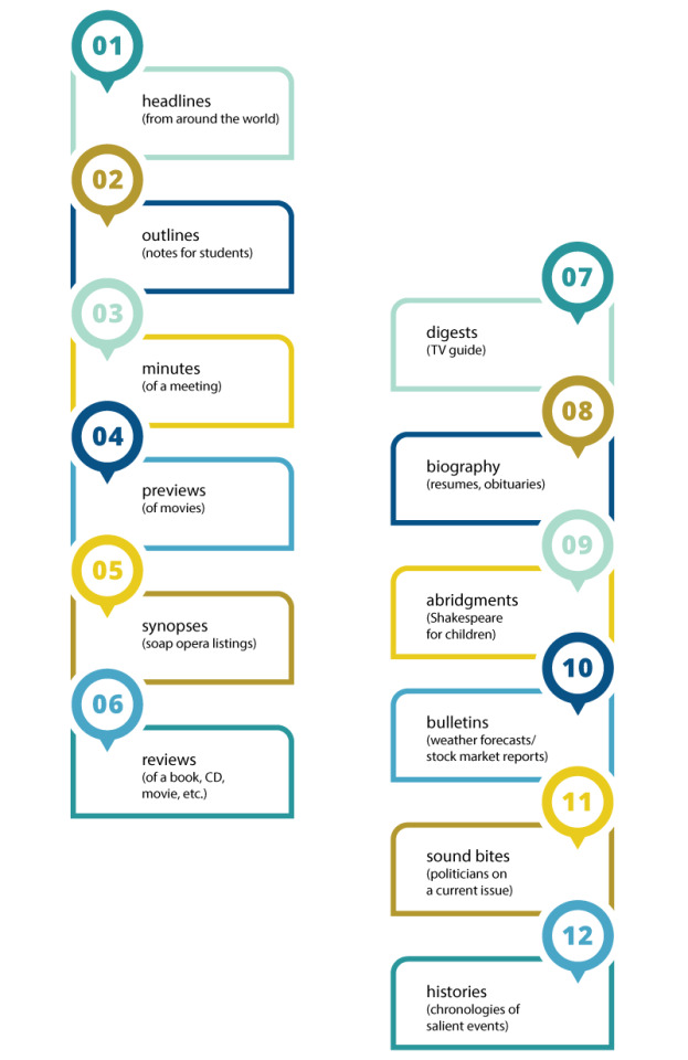
By now, the whole branch of natural language processing dedicated to summarization emerged, covering a variety of tasks:

· headlines (from around the world);

· outlines (notes for students);

· minutes (of a meeting);

· previews (of movies);

· synopses (soap opera listings);

· reviews (of a book, CD, movie, etc.);

· digests (TV guide);

· biography (resumes, obituaries);

· abridgments (Shakespeare for children);

· bulletins (weather forecasts/stock market reports);

· sound bites (politicians on a current issue);

· histories (chronologies of salient events).

The approaches to text summarization vary depending on the number of input documents (single or multiple), purpose (generic, domain specific, or query-based) and output (extractive or abstractive).

Extractive summarization means identifying important sections of the text and generating them verbatim producing a subset of the sentences from the original text; while abstractive summarization reproduces important material in a new way after interpretation and examination of the text using advanced natural language techniques to generate a new shorter text that conveys the most critical information from the original one.

Obviously, abstractive summarization is more advanced and closer to human-like interpretation. Though it has more potential (and is generally more interesting for researchers and developers), so far the more traditional methods have proved to yield better results.

That is why in this blog post we’ll give a short overview of such traditional approaches that have beaten a path to advanced deep learning techniques.

By now, the core of all extractive summarizers is formed of three independent tasks:

1) Construction of an intermediate representation of the input text

There are two types of representation-based approaches: topic representation and indicator representation. Topic representation transforms the text into an intermediate representation and interpret the topic(s) discussed in the text. The techniques used for this differ in terms of their complexity, and are divided into frequency-driven approaches, topic word approaches, latent semantic analysis and Bayesian topic models. Indicator representation describes every sentence as a list of formal features (indicators) of importance such as sentence length, position in the document, having certain phrases, etc.

2) Scoring the sentences based on the representation

When the intermediate representation is generated, an importance score is assigned to each sentence. In topic representation approaches, the score of a sentence represents how well the sentence explains some of the most important topics of the text. In indicator representation, the score is computed by aggregating the evidence from different weighted indicators.

3) Selection of a summary comprising of a number of sentences

The summarizer system selects the top k most important sentences to produce a summary. Some approaches use greedy algorithms to select the important sentences and some approaches may convert the selection of sentences into an optimization problem where a collection of sentences is chosen, considering the constraint that it should maximize overall importance and coherency and minimize the redundancy.

Let’s have a closer look at the approaches we mentioned and outline the differences between them:

Topic Representation Approaches

Topic words

This common technique aims to identify words that describe the topic of the input document. An advance of the initial Luhn’s idea was to use log-likelihood ratio test to identify explanatory words known as the “topic signature”. Generally speaking, there are two ways to compute the importance of a sentence: as a function of the number of topic signatures it contains, or as the proportion of the topic signatures in the sentence. While the first method gives higher scores to longer sentences with more words, the second one measures the density of the topic words.

Frequency-driven approaches

This approach uses frequency of words as indicators of importance. The two most common techniques in this category are: word probability and TFIDF (Term Frequency Inverse Document Frequency). The probability of a word w is determined as the number of occurrences of the word, f (w), divided by the number of all words in the input (which can be a single document or multiple documents). Words with highest probability are assumed to represent the topic of the document and are included in the summary. TFIDF, a more sophisticated technique, assesses the importance of words and identifies very common words (that should be omitted from consideration) in the document(s) by giving low weights to words appearing in most documents. TFIDF has given way to centroid-based approaches that rank sentences by computing their salience using a set of features. After creation of TFIDF vector representations of documents, the documents that describe the same topic are clustered together and centroids are computed — pseudo-documents that consist of the words whose TFIDF scores are higher than a certain threshold and form the cluster. Afterwards, the centroids are used to identify sentences in each cluster that are central to the topic.

Latent Semantic Analysis

Latent semantic analysis (LSA) is an unsupervised method for extracting a representation of text semantics based on observed words. The first step is to build a term-sentence matrix, where each row corresponds to a word from the input (n words) and each column corresponds to a sentence. Each entry of the matrix is the weight of the word i in sentence j computed by TFIDF technique. Then singular value decomposition (SVD) is used on the matrix that transforms the initial matrix into three matrices: a term-topic matrix having weights of words, a diagonal matrix where each row corresponds to the weight of a topic, and a topic-sentence matrix. If you multiply the diagonal matrix with weights with the topic-sentence matrix, the result will describe how much a sentence represent a topic, in other words, the weight of the topic i in sentence j.

Discourse Based Method

A logical development of analyzing semantics, is perform discourse analysis, finding the semantic relations between textual units, to form a summary. The study on cross-document relations was initiated by Radev, who came up withCross-Document Structure Theory (CST) model. In his model, words, phrases or sentences can be linked with each other if they are semantically connected. CST was indeed useful for document summarization to determine sentence relevance as well as to treat repetition, complementarity and inconsistency among the diverse data sources. Nonetheless, the significant limitation of this method is that the CST relations should be explicitly determined by human.

Bayesian Topic Models

While other approaches do not have very clear probabilistic interpretations, Bayesian topic models are probabilistic models that thanks to their describing topics in more detail can represent the information that is lost in other approaches. In topic modeling of text documents, the goal is to infer the words related to a certain topic and the topics discussed in a certain document, based on the prior analysis of a corpus of documents. It is possible with the help of Bayesian inference that calculates the probability of an event based on a combination of common sense assumptions and the outcomes of previous related events. The model is constantly improved by going through many iterations where a prior probability is updated with observational evidence to produce a new posterior probability.

Indicator representation approaches

The second large group of techniques aims to represent the text based on a set of features and use them to directly rank the sentences without representing the topics of the input text.

Graph Methods

Influenced by PageRank algorithm, these methods represent documents as a connected graph, where sentences form the vertices and edges between the sentences indicate how similar the two sentences are. The similarity of two sentences is measured with the help of cosine similarity with TFIDF weights for words and if it is greater than a certain threshold, these sentences are connected. This graph representation results in two outcomes: the sub-graphs included in the graph create topics covered in the documents, and the important sentences are identified. Sentences that are connected to many other sentences in a sub-graph are likely to be the center of the graph and will be included in the summary Since this method do not need language-specific linguistic processing, it can be applied to various languages [43]. At the same time, such measuring only of the formal side of the sentence structure without the syntactic and semantic information limits the application of the method.

Machine Learning

Machine learning approaches that treat summarization as a classification problem are widely used now trying to apply Naive Bayes, decision trees, support vector machines, Hidden Markov models and Conditional Random Fields to obtain a true-to-life summary. As it has turned out, the methods explicitly assuming the dependency between sentences (Hidden Markov model and Conditional Random Fields) often outperform other techniques.

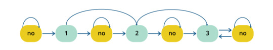
Figure 1: Summary Extraction Markov Model to Extract 2 Lead Sentences and Additional Supporting Sentences

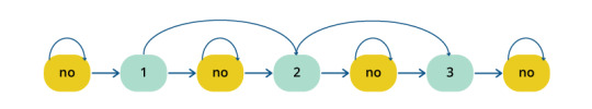
Figure 2: Summary Extraction Markov Model to Extract 3 Sentences

Yet, the problem with classifiers is that if we utilize supervised learning methods for summarization, we need a set of labeled documents to train the classifier, meaning development of a corpus. A possible way-out is to apply semi-supervised approaches that combine a small amount of labeled data along with a large amount of unlabeled data in training.

Overall, machine learning methods have proved to be very effective and successful both in single and multi-document summarization, especially in class-specific summarization such as drawing scientific paper abstracts or biographical summaries.

Though abundant, all the summarization methods we have mentioned could not produce summaries that would similar to human-created summaries. In many cases, the soundness and readability of created summaries are not satisfactory, because they fail to cover all the semantically relevant aspects of data in an effective way and afterwards they fail to connect sentences in a natural way.

In our next post, we’ll talk more about ways to overcome these problems and new approaches and techniques that have recently appeared in the field.

[mathematicianadda]

Returning to CSE maths 4 years after High School

I know this subreddit says that questions about "learning maths" should be on r/learnmath but I feel that my question is a little more focused (not just about...wanting book or resources) and could be answered here. Nevertheless, I will be posting this on there too.

​

This is a long one... bear with me. If you will.

​

I am going into the second year of a Computer Science degree and we have a course called "Engineering Mathematics" (ME3) in the next semester.

I graduated high school a WHILE ago and honestly need a little brushing up before I start learning ME3. But I don't have the time to go through all the maths topics we had then in all the 4 years. I was wondering if someone could help me decide what I should revisit and revise before going on to ME3.

Course Content of ME3

------------------------------------

1 - Linear Differential Equations (LDE)

\- LDE of nth order with constant coefficients \- Method of variation of parameters \- Cauchy's & Legendre's LDE \- Simultaneous & Symmetric Simultaneous DE \- Modelling of Electric Circuits

​

2 - Transforms

\- Fouriers Transform \- Complex exponential form Fourier series \- Fourier Integral Theorem \- Fourier Sine & Cosine Integrals \- Fourier Sine & Cosine transforms & their inverses \- Z Transform (ZT) \- Standard Properties \- ZT of standard sequences & their inverse

3 - Statistics

\- Measures of Central tendency \- Standard deviation, \- Coefficient of variation, \- Moments, Skewness and Kurtosis \- Curve fitting: fitting of straight line \- Parabola and Related curves \- Correlation and Regression \- Reliability of Regression Estimates.

​

4 - Probability and Probability Distributions

\- Probability, Theorems on Probability \- Bayes Theorem, \- Random variables, \- Mathematical Expectation \- Probability density function \- Probability distributions: Binomial, Poisson, Normal and Hypergometric \- Test of Hypothesis: Chi-Square test, t-distribution

​

5 - Vector Calculus

\- Vector differentiation \- Gradient, Divergence and Curl \- Directional derivative \- Solenoid and Irrigational fields \- Vector identities. Line, Surface and Volume integrals \- Green‘s Lemma, Gauss‘s Divergence theorem and Stoke‘s theorem

​

6 - Complex Variables

\- Functions of Complex variables \- Analytic functions \- Cauchy-Riemann equations \- Conformal mapping \- Bilinear transformation \- Cauchy‘s integral theorem & Cauchy‘s integral formula, \- Laurent‘s series, and Residue theorem

​

-------------------------------------------------------------------------------------------

Overview of roughly what all we had in the years of High School, a little out of order because I am summarizing all 4 years of Math books.

Real Numbers

\- Laws of Exponents for Real Numbers \- Euclid’s Division Lemma \- Fundamental Theorem of Arithmetic

​

Polynomials

\- Polynomials in One Variable \- Zeroes of a Polynomia, Remaider Theorem, Factorization of Polynomials \- Relationship between Zeroes and Coefficients of a Polynomial \- Division Algorithm for Polynomials

​

Pair of Linear Equations in Two variables

\- Linear Equations \- Solution of a Linear Equation \- Pair of Linear Equations in Two Variables \- Graphical Method of Solution of a Pair of Linear Equations \- Substitution Method, Elimination Method & Cross-Multiplication Method

​

Principles of Mathematical Induction

​

Complex Numbers

\- Modulus and the Conjugate \- Argand Plane and Polar Representation

​

Quadratic Equations

\- Factorisation & Completing the Square, Roots of Equations.

​

Sets----------

\- Sets: Empty, Finite, Infinite, Equal, Subsets, Power Set, Universal Set. \- Venn Diagrams \- Union, Intersection & Complement of a Set

​

Permutations and Combinations

​

Binomial Theorem

\- Binomial Theorem for Positive Integral Indices \- General and Middle Terms

​

Sequences and Series

\- Sequences & Series \- Arithmetic Progressions \- nth Term of an AP, Sum of n terms of an AP \- Geometric Progression \- Relationship Between Arithematic Mean and Geometric Mean

​

Matrices

\- Types & Operations \- Transpose \- Symmetric and Skew Symmetric Matrices \- Transformation \- Invertible Matrices

​

Determinants

\- Properties of Determinants \- Area of a Triangle \- Minors and Cofactors \- Adjoint and Inverse of a Matrix \- Applications of Determinants and Matrices

​

Relations and Functions

\- Cartesian Product of Sets \- Relations & Functions \- Composition of Functions and Invertible Function \- Binary Operations

​

Limits and Derivatives

\- Limits, Derivatives \- Limits of Trigonometric Functions \- Applications: Rate of Change of Quantities, Increasing and Decreasing Functions

Tangents and Normals, Approximations & Maxima and Minima

​

Continuity and Differentiability

\- Exponential and Logarithmic Functions \- Logarithmic Differentiation \- Derivatives of Functions in Parametric Forms \- Second Order Derivative \- Mean Value Theorem

​

Integrals

\- Inverse Process of Differentiation \- Methods of Integration \- Integration by Partial Fractions & by Parts \- Definite Integral \- Fundamental Theorem of Calculus \- Definite Integrals by Substitution \- Properties of Definite Integrals \- Applications: Area under Simple Curves, Area between Two Curves

​

Differential Equations

\- Basic Concepts \- General and Particular Solutions of Differential Equation \- Differential Equation whose General Solution is given \- Methods of Solving First order, First Degree Differential Equations

​

Vector Algebra

\- Types of Vectors \- Addition of Vectors, Multiplication of a Vector by a Scalar \- Product of Two Vectors

​

Linear Programming

​

Statistics

\- Graphical Representation \- Distribution. Mean, Mode & Median \- Measures of Dispersion, Range, Mean Deviation \- Variance and Standard Deviation

​

Probability

\- Random Experiments, Events, Axiomatic Approach to Probability \- Conditional Probability , Multiplication Theorem, Independent Events \- Bayes' Theorem \- Random Variables and their Probability Distributions \- Bernoulli Trials and Binomial Distribution

​

​

------------------------------------------------------------------------------

Euclids's Geometry

Properties of Lines, Angles, Circles, Triangles, Quadrilaterals, Parallelograms (Too easy to worry about)

Some chapters about Areas & Volumes of Quadrilaterals, Circles, Cylinders, Cuboids & Spheres (Again.. too easy)

​

Heron's Formula

\- Area of a Triangle – by Heron’s Formula \- Application of Heron’s Formula

Trigonometry

\- Trigonometric Ratios, Identities \- Applications : Heights and Distances

​

Trigonometric Functions

\- Sum and Difference of Two Angles \- Trigonometric Equations \- Inverse Trigonometric Functions & their Properties

​

Circles

\- Tangent to a Circle

​

Straight Lines

\- Slope of a Line \- Forms of Equations of a Line \- Distance of a Point From a Line

​

Conic Sections

\- Cone, Circle, \- Equations: Parabola, Ellipse & Hyperbola \- Eccentricity, Latus rectum

​

Three Dimensional Geometry

\- Coordinate Axes and Coordinate Planes in 3D Space \- Coordinates of a Point in Space \- Distance between Two Points \- Section Formula \- Direction Cosines and Direction Ratios of a Line \- Equation of a Line in Space, Angle between Two Lines, Shortest Distance between Two Lines \- Plane \- Coplanarity of Two Lines \- Angle between Two Planes \- Distance of a Point from a Plane \- Angle between a Line and a Plane

------------------------------------------------------------------------------------------------------------------------------------------------

Some of the topics are obvious. Like the entire Calculus section from "Relations & Function" to "Integrals" & Vector Algebra.

And Stats and Probability.

But what about Binomial Theorem, Sequences & Series, Matrices & Determinants. And Complex Numbers.

Polynomials, Quadratics is fairly easy.

And what about he Geometry-ish section. Especially the entire Conic Sections and 3D Geometry. I am completely blanked on that. I can't remember it at all.

I can remember a fair amount of Trig and Straight Lines (Slope & distance etc). Not sure if that is needed. Trig Functions is probably important. (sine, cosine etc)

Thank very very much for even taking the time to read.

submitted by /u/BhooshanAJ [link] [comments] from math http://bit.ly/2IHjCqL from Blogger http://bit.ly/2IsYvt1

[caseinpoints]

White paper: SCADA patterns & best practices, utility scale PV solar power plant control

Below is the overview from the white paper “SCADA Patterns & Best Practices, Utility Scale PV Solar Power Plant Control,” from NLS Engineering. Read the full white paper here.  

Photovoltaic (PV) cells have seen popular use for decades in household electronics such as calculators, battery chargers and emergency radios. PV generation is easily expandable. Single cells produce a small amount of DC voltage at their terminals and can be connected in series and parallel until their total combined output reaches the required capacity.

With modern technology, PV generation has become so efficient it is often the most cost-effective option for utility-scale production.

In a utility scale system, PV cells numbering in the millions are methodically stacked into groups connected in both series and parallel. These ordered panels are referred to as strings. Together their combined output of DC voltage and current can be used to produce a significant amount of power.

By their very nature, PV cells produce a DC voltage. DC voltage is not compatible with the grid, and that is where inverters become an integral part of a solar power plant. The fundamental role of an inverter is to convert the DC power derived from sunlight into AC power compatible with the grid. Modern-day plant controllers are designed to collect feedback from the grid and will adjust plant output to provide voltage support and frequency support.

This quality controlled AC power output is collected and combined from many inverters. Like any other utility-scale system, the output is stepped-up and distributed through a substation.

A PV plant requires many inverters to process the output of multiple arrays. Each inverter is capable of individual control functions but must coordinate, as a unified regiment, to appear as a single source at the Point of Interconnect (POI). This becomes the fundamental role of the plant controller. A power plant controller receives input from authorised users, sensory devices, and feedback applying this constant stream of data to established system directives. The controller commands the regiment of inverters as well as supporting capacitive and inductive devices to maintain the most stable and useful output possible. This document will describe the typical design, requirements and best practices when implementing a PV Plant controller.

The power triangle A thorough understanding of AC power fundamentals and the power triangle is essential to understanding grid-tied PV plant control. The necessity to invert DC (Direct Current) to AC (Alternating Current) presents the issue of power quality. Unlike DC (Direct Current), AC (Alternating Current) oscillates at a specified frequency causing current to switch directions regularly. Each time the direction changes, electromagnetic fields from inductors need to collapse and re-form in the opposite direction. Likewise, capacitors discharge and re-charge with an opposite polarity. This dynamic behaviour causes a phase-shift where voltage and current become out of phase from one another. In an ideal system, voltage and current would be synchronised, but in real-world applications, this is rarely the reality.

Inductive loads must establish an electromagnetic field before current flow occurs. If current and voltage waveforms were plotted together, the voltage would peak before the current. The current lags the voltage in its alternation from peak to peak. Capacitive loads cannot actualize a voltage differential until they have become saturated. Opposite to an inductive phase shift, a waveform plotting current would begin to flow before voltage begins to alternate. The current flows first, leading the voltage. The left waveform in “Figure 2 – Unsynchronized/Synchronized Waveform” is a graphical representation of a perfectly synchronised waveform. Current and voltage peak and pass the origin at the same times. The image on the right is an example of an unsynchronized wave. In this case, the voltage passes the origin before the current does. This is an example of current lagging behind voltage, caused by an inductive load.

The capacitive and inductive shifts are inversely proportional. As the effects of the properties on the phase shift counteract each other degree by degree, like integers on a scale, only the cumulative result will have an apparent effect on the phase shift. Therefore, one can be used to cancel the effects of the other.

The energy used by inductors/capacitors does not perform ‘useful work’ meaning that it does not directly contribute to the output power of the device. This component of energy is called reactive power, measured in volt-amps reactive (VARs) denoted by the letter Q. If the product of current and voltage is taken as an attempt to calculate power as one would for DC, it will include the non-useful reactive power component and not be truly representative of the ‘useful’ power. This measurement is called apparent power (S) and measured in volt-amps (VA). The component of useful energy is measured in watts (W) and described by the letter P.

The ratio of the active power (“P”, measured in watts (W), the voltage and current which performs real work) to the apparent power (“S”, measured in Volt-Amps (VA), The voltage and current applied to the circuit) depicts the efficiency of a circuit. As the phase shift shrinks, and the apparent power and the real power correlate, the ratio between them approaches 1. At a power factor of 1, 100% of the power (S) applied to a circuit is performing work (P). Realistically, there will always be a small inductive presence in a circuit, as the flow of alternating power through any conductor produces electromagnetic flux. 0.98 is a practical example of high efficiency.

The power factor relationship is commonly represented by a right-angle triangle.

As seen in “Figure 4- Power Triangle,” the angle formed between the active power (P) and apparent power (S) of a circuit is the phase angle (θ). The triangle expresses the complex magnitude of reactive power (“Q,” VARs), a measure of the power required to overcome the impedance in the system.

The power factor triangle is an excellent tool for understanding the relationships between active power, reactive power, apparent power, phase angle and power factor. Power factor, the percent efficiency of real power, is the cosine of the phase angle.

Most modern inverters are capable of simultaneously controlling both active power and reactive power individually while the total output does not exceed the apparent power rating of the inverter. Controlling Reactive Power(Q) of a PV plant is an important system directive which is comprehensively addressed in Automatic Voltage Regulation (AVR).

Control system architecture An optimal PV plant appears to the grid as a single unified source of power while maximising active power output and providing grid support. This is accomplished by balancing two modes of operation: Active Power Control (APC), and Automatic Voltage Regulation (AVR). Co-ordination between generator owners and system planners is crucial to a balanced grid. It is important to regulate the allowable amount of power at the Point of Interconnect (POI). Active Power Control (APC) limits generation at the POI to predetermined setpoints. This purposeful limitation is called Curtailment. Grid support through Automatic Voltage Regulation (AVR) is done by regulating reactive power.

Figure 5 shows a simplified control loop for plant control. The source of the plant-level setpoint may be one of the multiple authorised users. Local or remote, a plant operator or a collaborative body (ex. system operator), one source is selected at a time to direct the plant controller. Changes in setpoint from a user are passed to the PID controller through a velocity limiter.

The PID controller constantly compares the current setpoint with the actual value as it appears on the grid. This is what is referred to as a closed-loop feedback. Discrepancies between the current setpoint and instantaneous output at the POI manifest as an error which is used to correct the output. If the change in setpoint is too extreme, the output will overshoot the setpoint before it has the time to correct itself. To prevent operator induced overshoot or transients from setpoint changes, a velocity limiter transitions to the new setpoint gradually.

Each inverter is equipped with a controller that provides localised closed-loop control based on its commanded setpoints. The local inverter’s controller is constantly communicating with the plant controller. If an inverter stops communicating with the plant controller, it would appear offline or unavailable and omitted from plant control scheme. An inverter may still run and produce power even if it is unable to communicate with the controller. This emphasises the importance of a closed loop control scheme. Closed-loop feedback at the POI detects the unknown contribution and scales back the commanded output to compensate.

Unlike traditional generators, the prime mover or fuel source is often uncontrollable for renewable resources. With PV generation, weather and sunlight conditions cannot be controlled. Irradiance may be too low or irregular for the plant to meet the demand. Similarly, partial cloud cover can affect different areas of the plant disproportionally causing the output to fluctuate. The closed loop nature of the PID allows the plant controller to provide partial compensation by increasing the requested setpoint to all inverters. Inverters which are affected by cloud cover will only be able to produce the power available from their limited irradiance, but other inverters can produce more than their fair share to compensate.

To prevent overshoot during a rapid increase in irradiance, anti-windup techniques are used to limit PID output during low irradiance. Additional techniques such as inverter ramp-rate control can be used to control changes in plant output.

The center of the plant controller is a PLC that constantly monitors data from all areas of the plant, compares real-time data with operator instructions and relays commands back to plant devices. The controller aggregates information from the POI (Point of Interconnect), relays and meters, meteorological stations (MET stations), capacitor banks, and every individual inverter. The information is used by the controller in conjunction with instructions from the operator to command plant level changes to setpoints.

Manual control Occasionally, it becomes necessary to isolate a single inverter from the collective service. A plant controller should have the ability accommodate this request by placing an inverter into a PLC-Manual Control mode. Once in ‘PLC-manual’, the inverter will be separate from the control scheme; it will no longer be regulated by the main control loop.

The inverter’s output will remain included in the curtailment calculations at the POI (Point of Interconnect).

As soon as the mode is changed from automatic to manual, the inverter should maintain its last set of setpoints received in automatic. This provides a smooth changeover between manual and automatic modes. The operator can then specify setpoints on the screen to be written directly to the inverter. The setpoints are checked to ensure that they do not exceed the capability of the inverter. While in manual, an inverter can be shut down and taken out of service.

The plant control scheme should consider KW and KVAR contribution from an inverter which is running in manual mode and be versatile and adaptive enough to compensate for lost control by shifting the remaining load to the available inverters. Despite the best efforts of the controller, if too many inverters are placed in manual the controller will not have the resources to compensate and the operator will lose consistent control.

If an inverter needs to be shut down and taken out of service, it should be done so from the HMI. It is not ideal to place an inverter into manual or shut it down at the inverter because it will simply appear to the controller as though it has lost communication with that inverter. Place the inverter into PLC-manual, and then issue a stop command. This will incrementally reduce the output of the inverter until it is low enough to be brought to a full stop. Once the inverter is shut down, follow proper shutdown and lockout procedures from the manufacturer.

Read the full white paper here. 

The post White paper: SCADA patterns & best practices, utility scale PV solar power plant control appeared first on Solar Power World.

[runewake2]

Dot products are extremely useful for a whole number of tasks. In this video we're going to look at applying them in a way that will allow us to detect which side of a dice is facing up. This will allow us to use rigidbodies to simulate rolling a dice and get the result no matter what the shape of the dice. We can simulate a d20, d6, even a coin flip with this technique. Dot Products are a mathematical function that returns a value based on a the alignment of two vectors. Two normalized vectors parallel to themselves and heading in the same direction give a dot product of 1. Perpendicular normalized vectors give a 0 and parallel vectors in opposing directions result in -1. The actual value is related to the inverse cosine of the angle difference between the two. Hint: The Arccos(X) where X is the dot product of two normalized vectors returns the angle between the two vectors. We don't use this here, but it's a pretty neat trick! Our solution creates a list of vectors in local object space that determine which direction the sides are facing. Once we have that we translate each vector from local space to world space using the Dice's Transformation Matrix (localToWorldMatrix). This gives us a vector for each side in world space. Now that we have that we can determine which of the vectors has the greatest dot product when compared against the tables up direction (Vector3.up). That vector is our currently selected dice side. You can get the dice roller script on GitHub here: http://ift.tt/2qf4o01

[dariosanfilippo]

The best compromise for the design of a time-variant 1-pole filter in Pure Data

These days, I’m trying to turn pretty much anything into a time-variant system so here is my experience with a 1-pole filter. What follows is a short blog post on a couple of days of work where I have experimented with different designs to find the best compromise for a filter whose cutoff frequency can be piloted by signals.

A 1-pole filter, which is called so because it has one resonance, is described by the following difference equation:

y[n] = a * x[n] + b * y[n - 1].

y[n] is the output, a is the input coefficient, x[n] is the input, b is the feedback coefficient, y[n - 1] is the output one sample in the past.

The sign of the feedback coefficient determines the type of the filter and the position of the pole in the spectrum. Positive values result in a low-pass (LP) with a resonance at 0Hz; negative values result in a high-pass (HP) with a resonance at Nyquist, which is half the samplerate (SR).

In order for the filter to be stable, the absolute value of the feedback coefficient must not exceed 1, and the input coefficient is calculated as 1 - |b| so that we have unity gain at the pole.

The cutoff of a filter is defined as the frequency at which the input is attenuated by about 3.01dB.

The larger the feedback coefficient, the closer the cutoff of the filter will be to its pole. Of course, the relationship between the cutoff and the feedback coefficient is nonlinear, so this is the tricky aspect of the design of this filter.

Let’s consider the LP type.

To determine whether the coefficient calculation is accurate or not, we can tune in the cutoff of the filter and the frequency of a sinusoid that we use as input. Then, we can calculate the RMS and see if the attenuation is as expected. We will consider a good frequency response anything within a +/- 3% error from the expected attenuation.

The first experiments that I performed were using the implementation from the Audio Programming book by Boulanger and Lazzarini. The equation for the calculation of the coefficients uses trigonometric functions and is the following:

sqrt((2 - cos(w))^2 - 1) - 2 + cos(w)

where w is the angular frequency defined as 

2 * π * f_Hz / SR.

Please note that the design above produces negative coefficients. That is because they have based the design on a difference equation prototype with a negative sign for the feedback coefficient, so the coefficients would flip back into positive values.

The frequency response of a digital filter is dependent on the SR, so we can use the normalised frequency (let’s call it f_n) defined as

f_Hz / SR

to have a unit which consistently describes the system regardless of its SR. Given that the maximum frequency in a digital system is Nyquist, the normalised frequency will be in the [0;.5] range.

With the design described above, the filter implemented in Pure Data Vanilla has a good frequency response from about .000010721 (~4.7281Hz at 44.1kHz SR) all the way up to .5 (Nyquist), although the closer we get to the lower value, the more the coefficients produce a staircase and there is less resolution for the fractional part of the cutoff. Below the lower value, the response of the filter worsens and the coefficients are clipped to 1 after ~.000067303 (~2.96807Hz) is reached, meaning that from that point downward the filter will just output DC (0Hz).

Another design that I tried and which also uses trigonometric functions is that from Cliff Sparks. The formula that he uses is the following:

2 - cos(w) - sqrt((cos(w) - 3) * (cos(w) - 1)).

This filter behaves very similarly to the one from Boulanger and Lazzarini, although the cutoff after which the coefficients are clipped to 1 is here .0000389273 (~1.7167Hz).

Miller Puckette in his implementation uses a formula that is an approximation:

1 - w

where w, like we said above, is the angular frequency.

That is a computationally very efficient calculation which actually has a rather good behaviour in the very low frequency range, roughly from .00000023692 (~.0104Hz at 44.1kHz) -- which is the largest possible coefficient before unity in PD (.999999) -- up to .00644731 (~284.326Hz). Though, the coefficients need to be clipped to 0 after ~.15915 or they would result in negative values.

After a look online, I found a blog post from Nigel Redmon who proposes the implementation from the book Musical Applications for Microprocessors by Hal Chamberlin. On a comment, Nigel also described the reasoning of the author of the book who proposed this implementation:

“He notes that a one-pole filter is a leaky integrator, which is equivalent to an analog R-C low-pass filter. He also notes that it’s well-known that capacitor voltage discharge follows an inverse exponential curve: E = E0exp(-T/RC), where E is the next voltage after period T, given the initial voltage E0, R and C are the resistor and capacitor values in ohms and farads. The cutoff frequency is defined by Fc = 0.5πRC; substituting we get E = E0exp(-2πFcT). The time change, T, is the sample rate in the digital system, so converting to sampling frequency, Fs = 1/T, we get E = E0exp(-2πFc/Fs). To adjust for a gain of 1 at DC (0 Hz), we set the input multiplier to 1 – that value.”

Fc is the normalised frequency (f_n), so the final formula for the coefficients is:

exp(-2 * π * f_n).

This is by far the best compromise as, like Puckette’s implementation, it has a very good response in the very low range while keeping a reasonably good response throughout the whole spectrum.

Are the formulae using trigonometric functions wrong? No. They would actually give the most accurate response in a different environment.

Pure Data is an amazing software: it is open-source, reliable and efficient, although the internal resolution is (yet) single-precision, and that results in inaccurate coefficients when using trigonometric functions. Besides, if one wanted to implement the filter in the audio domain, the cosine function ([cos~]) is based on a table and that would result in even less accurate values than those given by the message domain one ([cos]).

The math operators involved in Puckette’s and Chamberlin’s implementations are consistent in both the message and audio domains, so they are good candidates for the time-variant version of the filter.

Puckette’s formula is the least computationally expensive, so it is probably the best one if all you care is filtering in the very low range.

Chamberlin’s implementation involves a call to an exponential function but it is still a reasonable option considering that the filter would work for the entire spectral range.

And considering that flipping the sign of the feedback coefficient would flip the frequency response, a HP filter based on that implementation could easily be achieved by changing the sign of the coefficient while flipping the cutoff around the centre of the spectrum:

-exp(-2 * π * (.5 - f_n)).

[tutoroot]

What are the Steps to Create Values for Trigonometry Table?

The Trigonometric Table is essentially a tabular compilation of trigonometric values and ratio for various conventional angles such as 0°, 30°, 45°, 60°, and 90°, often with extra angles such as 180°, 270°, and 360° included. Due to the existence of patterns within trigonometric ratios and even between angles, it is simple to forecast the values of the trigonometry table and to use the table as a reference to compute trigonometric values for many other angles. The sine function, cosine function, tan function, cot function, sec function, and cosec function are trigonometric functions.

The trigonometric table is helpful in a variety of situations. It is required for navigating, research, and architecture. This table was widely utilized in the pre-digital age, even before pocket calculators were available. The table also aided in the creation of the earliest mechanical computing machines. The Fast Fourier Transform (FFT) algorithms are another notable application of trigonometric tables.

Steps to Create Values for Trigonometry Table

Step 1: 

Make a table with the top row showing the angles such as 0°, 30°, 45°, 60°, and 90°, and the first column listing the trigonometric functions such as sin, cos, tan, cosec, sec, cot.  

Step 2: Determine the value of sin 

To find the sin values, divide 0, 1, 2, 3, 4 by 4 under the root, in that order. Consider the following example. 

Step 3: Determine the value of cos 

The cos-value is the inverse of the sin angle. To find the value of cos, divide by 4 in the opposite order as sin. For example, to find cos 0°, divide 4 by 4 under the root. 

Step 4: Determine the value of tan 

Tan is defined as sin divided by cos. Tan equals sin/cos. Divide the value of sin at 0° by the value of cos at 0° to get the value of tan at 0°. 

Step 5: Determine the value of cot 

The reciprocal of tan is the value of cot. Divide 1 by the value of tan at 0° to get the value of cot at 0°. As a result, the value will be as follows: cot 0° = 1/0 = Unlimited or Not Defined  

Step 6: Determine the value of cosec 

The reciprocal of sin at 0° is the value of cosec at 0°. 

cosec 0° = 1/0 = Unlimited or Undefined 

Step 7: Determine the value of sec 

Any common values of cos may be used to calculate sec. The value of sec on 0° is the inverse of the value of cos on 0°.

While we learn trigonometric values of the trigonometry table, it will also be interesting to take note of the application areas of the table. On a broader note, the trigonometric table is used in:

Science, technology, engineering, navigation, science and engineering. Before the advent of the digital era, the trigonometric table was very effective. In the course of time, the table helped in the conceptualization of mechanical computing devices. Trigonometric tables are also used in the Fast Fourier Transform (FFT) algorithms.

The angle values of trigonometric functions, cotangent, secant, and cosecant are computed by applying these standard angle values of sine, cosecant, tangent. All the higher angle values of trigonometric functions such as 120°, and 360°, are easier to compute, through the standard angle values in a trigonometric values table. If you still can’t remember the values of Trigonometry tables, consider Tutoroot personalised sessions. Our experts will help you clearly understand the table along with tricks to memorize.