timothylo-blog

[timothylo-blog]

Woo! We made it. I’m still feeling a little under the weather, so I’m just going to follow the suggested prompts. Sorry for the lack of creativity.

I’m not sure if it qualifies as the most memorable moment, but the video above captures what may have been the most satisfying. Not only was it visually mesmerizing (I could have sat there all day just watching this, but we had other tests to run), but after all the problems we had with our dye, lighting, and the water channel itself, the payoff here was spectacular. 

I found the most challenging aspect of this course to be the seemingly never ending stream of technical problems. Having only really performed controlled lab experiments in physics and chemistry, where everything is planned by the professor and has been performed countless times before, I wasn’t really ready for the number of things that could go wrong in a real lab. But as I mentioned above, the gratification of finally overcoming all those challenges and getting good data made it all worth it.

I’m personally unsure of what the “environment in which I thrive” is anymore, but overall I feel much more comfortable dealing with all the aforementioned challenges of real lab work. As for the “no-single-answer” questions, I think this lab provided a lot of practice dealing with multi-factor problems. Throughout all the labs, we were constantly running into issues, be it with our apparatus, our data, or our analysis... Having to search for all the possible and most probable solutions to all these problems, I think we’ve all gotten better at hypothesizing causes and solutions for any sort of issue.

So, I kind of have a weird approach to team dynamics. I used to do a lot of leadership work, and have a fair bit of experience managing my peers, but I generally don’t like taking the lead. I’d rather follow one of my teammates’ lead and just deliver whatever I’m responsible for. Of course, this sometimes doesn’t go all that well... If it seems like the group isn’t actually getting anywhere, or our current leadership feels a little directionless, I’ll step in, but only a little bit. Nobody likes feeling like they’re being usurped, so I try to direct the group towards solution rather than simply taking over. Back in highschool I used to work as a tutor, and now I work as an instructional student assistant. Drawing on my experience in teaching, I’ll ask my entire group leading questions that should at least get us moving in the right direction again. That way, just as my students really do solve the problem on their own, our group leader maintains his/her position and we are set back on track. (That was a weird ramble... not sure if that even related to the question.)

I think that I’m somewhere in between on this one. While the course exposed me to something really cool that I had idea about, I don’t think experimental testing is something I could do every day. I feel that if I was constantly setting up and running tests like these, I would eventually burn out. If I was working on something else, and we had the opportunity to run some wind tunnel tests, I’d definitely be up for that... But I think I could only handle it in moderation. Living in the wind tunnel is certainly not for me.

I’m not really sure here. Perhaps inclusion of something in the water channel might be cool. This quarter only a small portion of the class actually was able to work with it. I don’t know what exactly we would do with it, since quantifying things is rather difficult with the current setup...

I think that the three little projects that we had in 302 were quite useful for developing the thought processes required for 307. The open-ended nature of the flow viz project at least starts forcing students to think for themselves. But something a little more structured like the atmospheric boundary layer report is probably the best option. Labs that have a very defined set of requirements but multiple ways to get there would prepare future students for the endless “no-single-answer” questions of 307.

I remember back in 331, Dr. K openned the course with a very long and confusing metaphor that was intended to show the importance of understanding the physical meaning of engineering problems. While that didn’t really help me at the time, I think that the idea is definitely important. In 301, 302, and 303 we studied from textbooks about all sorts of aerodynamic and thermodynamic phenomena, but we never really discussed what they physically were. I found that this lab didn’t really show me what the physical meanings were, but rather it forced me to put it all together myself. In order to figure out the issues we were seeing in our data, we had to put what we learned in previous classes into a physical perspective and analyze how it might be effecting our data.

Alright, I don’t really think I answered half of these questions... I just sort of prattled on about vaguely related things. 

[timothylo-blog]

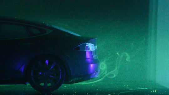
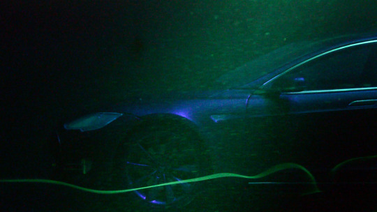
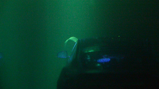
Welp, I had intended to post this yesterday, but I got sick and spent all day in bed... Anyways, on Friday we finally got solid data!

Conditions weren’t exactly optimal, but we did what we could. Apparently the filter was leaking slightly, so the previous group didn’t run it overnight. As such, the water channel was already slightly murky before we started testing, but this may have actually worked in our favor for a little while. Since there were a lot of tiny fluorescent particles in the water, we didn’t need to sort out any sort of normal lighting to make sure the car was visible. The fluorescence of the water provided more than enough light to see everything we wanted.

Initial setup took about half an hour. We dumped the previous dye mixture, and flushed out the tubing to get rid of any large particles leftover from our mishaps on Thursday. Then we remixed the dye with the original concentrations and hooked the bottle back up to the injection system. We also changed our light tent design to allow our cameraman to get in behind the channel. With the questionable use of a very expensive tripod and several chairs, we even raised the interior height of our tent to make testing more comfortable!

After that, we just ran through our original test matrix, and took a mixture of photographs and videos. As the tests went on, we moved to only taking videos, as the photos were coming out poorly. The pictures above are actually just frames snapshotted from our videos. Originally, we had planned to capture only a few phenomena, but with multiple camera angles. Due to visibility limitations (and the cloudiness of the water), we had to change our plan slightly. Instead of including extra camera angles for each area of interest, we incorporated more test locations to compensate.

We’re still finishing our memo to Kevin, but we’ll be wrapping that up Monday. I can’t say too much about that since it’s not done... So on to overall reflections!

[timothylo-blog]

Murphy’s Law...

So on Thursday sat down after lab and wrote a post about how everything went wrong during the past week. Then I packed up my laptop to go to another class, and forgot to save my draft... So here we go again:

Testing in the water channel this week has been rough to say the least. Since the channel was removed on Friday for the ME Senior Showcase, technical difficulties seem to have sprung up as often as leaks.

First, the channel itself was not reinstalled properly. When we arrived to the lab on Tuesday, excited to test out the dye mixture and splitter plate we’d spent the previous week preparing, we found another water channel group hard at work plumbing an empty channel. As it turns out, they had planned to test over the weekend but they were still working on remedying the reinstallation mishaps. Between the two groups, we widened the table, permanently attached the inlet flow connection, realigned the plumbing (several times), installed a new filter, and finally got the water channel working on Thursday.

Before we started our tests, we knew that proper lighting would be vital to capturing high quality images. Using two UV flashlights (torches), our phone lights, paper towels, black paper, the wooden water channel cover, the laser screen, and two tarps, we tried various setups to optimize light over the model. Fiddling with all these and erecting a makeshift tent, to block out as much light interference as possible, took the greater part of our 3-hour testing period.

When we settled on a setup that provided enough light to see the model and the fluorescent dye simultaneously, we found that the dye concentration was too low. Thus began the very frustrating dye debacle. Replicating the method we tested the week before, we mixed equal parts of dye and olive oil in a cup. Then we added that mixture to the dye bottle and filled the rest with water. From previous tests, we expected that the solution would remain intact for about two hours (more than enough time to finish our test). But after no more than 10 minutes, the dye injected into the channel began separating. Little blobs of dye accumulated on the splitter plate and on the rear window of the model, and bits of olive oil floated up to the surface. It was impossible to get a streamlight of dye and the channel gradually became cloudier. We kept having to shake up the dye bottle and clean up excess dye. Eventually, it became so bad that we just stopped testing for the day and changed the filter instead.

We met again today to finish our test, and it went a lot smoother. It may have been the longest spill-free water channel test all quarter. We’re still putting together our images, so I’ll probably post about it tomorrow.

[timothylo-blog]

Progress, sweet progress!

This week we actually accomplished quite a bit. Despite the fact that the water channel is currently empty, we have pretty much everything set up to start testing on Tuesday.

Splitter Plate: We found a piece of scrap aluminum behind the wind tunnel and cut out a 18″ x 7.25″ section. Once we add a little bit of rubber adhesive to the edges to protect the acrylic, this should perfectly span the channel. So far we’ve primed and painted the entire plate with a black semi-gloss spray paint. Over the weekend we plan to sand down the surface a little, to make the finish less reflective. We also will finish 3D printing the last 2 supports and epoxy them to the plate.

Fluorescent Dye: After cleaning out the previous dye bottles (which was not a short job), we attempted to dilute our new fluorescent dye in water... And found that it just sort of clumps into a bead and sinks to the bottom of the bottle. So! At Dr. Doig’s suggestion we grabbed a gallon jug of olive oil from the wind tunnel and mixed it in equal parts with the dye. The resultant mixture actually mixed quite well with water and we were able to hook up the pressure valves to produce little fluorescent dye streams in a bucket of water. Nothing is certain until we can run the tests in the water channel, but for now we’re optimistic that this will work.

Carbon Filter: Dr. Doig kindly ordered us a new activated carbon filter that should be arriving by next week. Since it’s designed to fit into the same case as our current filter, replacing them should be relatively easy. We may run a few tests with the current paper filter to see if it will pick up the fluorescent dye, before changing the filters. But nothing is set in stone.

[timothylo-blog]

Our Enigmatic Fluorescent Dye

So, Dr. Doig purchased this Universal A/C Fluorescent Dye that’s designed to be used in air conditioning or automotive systems to locate leaks. We looked up the Material Safety Data Sheet (MSDS) on the manufacturer’s website. However, due to the proprietary ingredients, the MSDS actually provided very little information.

The dye is composed of two ingredients: a solute (the dye itself) and a solvent (which makes up the majority of the contents). After looking around the internet and finding several other MSDS for other fluorescent dyes, we determined that it is fairly likely that the dye is meant to be used with oil rather than water. On the manufacturer’s website, the product page states that it is “POE Ester based” and  recommends use of “1/4 oz per 12 oz oil”. We will be testing the dye this Tuesday to confirm this and ensure that we can still use it for our tests. If not, we have already started looking into some other fluorescent dyes, both water-based and mineral oil-based. 

In general the disposal recommendations have been vague: simply stating that local, state, federal, etc. regulations should be followed. After looking at the MSDS for similar products, the primary concern seems to be the concentration of color. Considering the amount of dye we will be using and the volume of water it will be diluted in, we concluded that the color concentration should not be a significant factor. Although the wastewater certainly won’t be safe for the drain, it should be sufficiently diluted for sewage disposal.

[timothylo-blog]

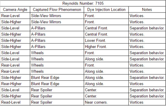
Also under Kevin’s recommendation, we made a little table to plan out what exactly we’re going to be looking for in our flow visualization. So we took a look at the different areas that we wanted to investigate and the different camera angles we could achieve... 

For the floor mounted splitter plate, we came up with these 15 tests to take a look at what we expected to see for each of the 5 areas of interest. In general, the phenomena we are looking to observe are either the wake vortices or the general path flow takes. 

The Reynolds number at the top is currently only an estimate. We used 2.1in/sec as a guess for what tunnel speed we’ll be running at, but this could change when we actually get into the lab. Garrett and Jacob used this speed when working with the vegetable-based dye, but we aren’t entirely sure if this will be optimal for the fluorescent dye. The other values in the calculation should remain relatively constant. For reference length, the width of the car model was used, since it is a bluff body rather than a streamlined one. And for the properties of water, we assumed that the temperature of the water is approximately room temperature. When we actually get to the lab, we’ll need to take readings to make sure that assumption is valid.

[timothylo-blog]

In order to move the model out of the floor boundary layer of the water tunnel, we were working on designing a testing table. 

Using SolidWorks, we created a splitter plate to sit in the bottom of the tunnel. But after meeting with Kevin, we’ve decided to go with a much simpler approach. We took the supports from this design and 3D printed those, and plan to affix them to a thin sheet of aluminum or possibly some scrap of carbon sheet. 

Currently, we have plans to at least get some flow visualization with the splitter plate, but we’re also trying to figure out how to get the model mounted sideways in the water tunnel. Due to the model being quite wide relative to the water channel test section, a side mount would likely reduce the effects of the sidewall boundary layers. However, we decided that it may be slightly risky to attempt the side mount first. In case that didn’t work out we still wanted to have something to show, so we’re doing the floor mounting first and designing the side mount in the meantime.

[timothylo-blog]

Lab Hack: Tesla Model Water Tunnel Flow Viz

Okay, so on to what we’re actually working on this week. Right now, we are just prepping for the tests and waiting for our “client” to come talk to us.

This should be a pretty cool test, but all we’ve done so far is research different elements of the test and write our proposal. I think I’ll separate the things we’ve been looking into into different posts... Sorry for the post blast... I wanted to make sure we had everything settled before putting these out.

[timothylo-blog]

Flow Viz: Tuft Testing

So, I sort of forgot to add posts last week for the tuft testing that we did... I guess I’ll just quickly reflect on a few things before moving on to the lab hack stuff.

We had chosen to use tufts under the assumption that it would be a relatively straightforward method and require minimal setup. We had hoped to maximize our tunnel time, allowing us to obtain more data to analyze. Unfortunately, adhering the tufts to the wings was a surprisingly long process. We had booked the tunnel from 1pm-3pm and three of us arrived at the tunnel at 11am to start working. Between cutting hundreds of 1.5″ pieces of yarn, preparing the wings, and arranging and taping the tufts on, the process took much longer than anticipated. 

After we finished the first wing, half of the group moved into the tunnel to setup the GoPro mount and DSLR tripod. But the force balance setup delayed testing for another hour, and by the time we could start testing the first wing, the second was fully tufted as well.We made the mistake of turning on the GoPro too early and its battery died during the last test. This turned out to not be a major problem because the force balance stepper broke during the same test. 

Despite all the technical issues with our actual tests, we actually managed to get pretty decent images to analyze. Since we already made our presentations, there’s no real point in recapping everything, but i guess I’ll review some of the improvements that we could make in future. This  was a picture in the last slide of our presentation that showed the wing after it was removed from the tunnel.

 And you could actually still see the same patterns that were exhibited while the wing was in the tunnel. This proved that the yarn we used for tufts was too stiff. We noted this fact while analyzing the lower angles of attack, because some of the tufts would remain in the same position from the end of the previous test. In the end, we managed to do some solid analysis, but it might be worth looking into different types of yarn for future tufts testing.

[timothylo-blog]

Reflections: Take 2

Here we go again:

Since I was the analysis lead for my group, I dealt with most of the data acquisition and reduction. Since we settled on a testing scheme early on, it was relatively easy to collate data sets for comparison. We stored all the Lab View data files from each week’s experiment in a separate folder and used a Matlab script tailored to that experiment to extract the performance characteristics we were looking for. I then created a system of Matlab structures that organized and stored the calculated values and their respective errors for each test and saved one for each experiment in a data consolidation folder. Then I wrote another script whose sole purpose was to compile the data and make it presentable. By the time we needed to write out report and make specific figures to point at, all we needed to do was change one vector in the script and we could specify exactly which tests we wanted to see data for. Then the script would group everything we asked for appropriately, take the averages, find the standard deviations, and plot them all as error bars. It also produced plots of each individual test case we requested with error bars based on the propagation of error from measurement. Overall, I feel like we handled the huge amount of data we collected fairly well. The only thing I feel like we could have added was a method to tabulate it all, so that it could be added as an appendix to the report... Unfortunately, the sheer amount of numbers we had made that impractical given the time we had.

I think that the analysis of why the numbers we measured/calculated didn’t line up with other sources was the most interesting part of the whole experience. Although a lot of my error considerations on tumblr were purely hypothetical, when we actually sat down with our numbers and wrote the paper, we were able to to make some more solid connections. We were actually able to use the aforementioned giant structures of standard deviations and error to identify regions in our alpha sweeps where the variability and accuracy of the data changed. This allowed us to quantitatively support our claims about certain turbulent and unsteady effects that were not necessarily evident from the plots or raw numbers.

We were one of the groups that was supposed to test with the force balance on Tuesday, when everything went haywire. So all of our finite wing data was acquired second hand. For the red wing, we were at least allowed to observe the group running the experiment and take notes on their procedure. Combining this with the data they provided us, we actually produced somewhat reasonable numbers. At the very least, they were close enough to make some sort of comparison with reference information. On the other hand, the blue wing tests were completed by an entirely different lab group and we only received their data after the fact. Unfortunately, we didn’t receive a tunnel off measurement after all the tests were completed, and were not able to accurately account for the load cell drift over the second test. Since we weren’t there to measure things ourselves, this was extremely frustrating to deal with. While we were responsible for and felt confident in the level of accuracy we found in our own data, we had no control over how the blue wing tests were conducted. As with the red wings, we found the obtainable performance characteristics, their error, averages, and standard deviations. However, for the data that we were actually responsible for, I felt that we did a relatively good job of analyzing and accounting for any oddities.

I actually only had to clamp/unclamps during the first week of testing on the infinite airfoil. It was very exciting. Though, I found that running the Matlab scripts and performing live analysis on any weird data points was much more interesting.

Being able to create our own lab procedure was actually a very fulfilling experience. While most labs provide detailed instructions for every little step and almost always produce results similar to expected value. When we had the opportunity to define our own procedure, and specify exactly what we were looking for, I felt much more invested in actually finding something. At the same time though, our inexperience in creating our own procedures led us to some questionable findings. Going from the first week to the second, we completely botched Reynolds number matching and made our later analysis even more difficult. Overall, the entire series of labs was most definitely a learning process. By the end of it all, I felt like we could redo the entire thing and get much better data. Of course, I think we’re all so burnt out and fed up with the 4412 that nobody would agree to it.

I think that the three biggest takeaways were:

To get as much data about everything that happened as possible. Photograph everything from every angle, measure everything, measure how everything was measured, record how exactly everything was done, etc...

To expect something to go wrong, because something always goes wrong. And dealing with it will make or break the data/analysis and the final report.

To fully plan out everything and agree to a testing scheme before starting. That would have prevented our Reynolds number issues... 

(PS: I tried to replicate the thoughts I wrote down earlier as quickly and accurately as possible. I don’t know how or why my post disappeared, but hopefully this makes it in on time.)

[timothylo-blog]

Tumblr threw my reflections away!

So, apparently tumblr did not post my reflections....

I’m rewriting everything now...

[timothylo-blog]

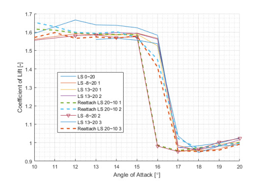
Breakdown of Low-Speed Tests

Since we wanted to have most of our infinite airfoil testing to be at a Reynolds number we could replicate and compare to the upcoming finite airfoil tests, we have a lot more data to look at here. Unfortunately, we also experimented with different angle of attack sweeps, making it difficult to compare all of the data at once. 

Though most of the tests follow the same trend in the Lift-Drag polar, there are a few oddities:

Two of the reattachment tests showed significant deviation from the rest of the data, while the third did not. The weird thing here is that we expected all of them to show a difference from the tests with ascending angle of attack. I really don’t know why, but the third test’s drag coefficient actually does correlate well with the other two test. The only significant difference occurs in the lift coefficient plot where it deviates from the other two tests, and oddly is even farther away from the increasing angle of attack tests.

Just like the reattachment tests, there was one normal test that was just weird.  For clarity, I added little triangles to this plot. In all three plots, this test almost exactly followed the odd reattachment test for a majority of the tested angles of attack. I went in and checked the numbers to make sure there wasn’t something going wrong with the variables, but it all checked out and the two problem tests were actually different (very slightly). 

The very last normal test, labeled “LS 13~20 3,” had a few odd data points near 15° (expected stall). This test saw a little increase in both lift and drag in this region, but was otherwise normal.

I honestly have no explanations for the first two bullet there. I first made these plots on Friday and have since mulled it over, but I can’t figure it out.

The last point though, we have a well recorded source of error. During the last two tests listed in the legend, we conducted a little bit of flow visualization with smoke. We wanted to take a look at how flow was behaving around the airfoil, and also the rake. The results of that are a whole nother post, but it’s possible that having one of our group members standing directly in front of the tunnel inlet affected our data.

[timothylo-blog]

Breakdown of High-Speed Tests

From the standard deviation plots, I noticed that the high speed tests actually had a very reasonable standard deviation throughout the range of angles of attack where we expected separation to occur. The only exceptions were the last two data points, at 19° and 20° angle of attack. To check more into this, I plotted all four of the high speed tests.

From the Lift-Drag polar, we can see that there are two distinct groupings. After checking back to see when each test was run, I found that the two solid line plots were taken before the wake rake was installed and the two dashed line plots were taken afterwards. 

It seems like the presence of the rake is having some sort of influence on our high speed data at higher angles of attack. From the lift coefficient plot, we can see that the characteristic drop off after the airfoil stalls is not present in the tests that included the rake. Instead, the plots begin a slow, linear decline from 16° to 20° angle of attack. Oddly, the drag coefficient shows that the very first test we conducted is the one that diverges from the group. I’m not entirely sure how to explain that.

The fact that the deviation from previous tests only occurred at high angles of attack during the high speed tests implies that the cause might be dependent on a viscous or blockage effect. The high speed tests were conducted at a higher Reynolds number than the rest of our testing, and were limited in number because they would be impossible to recreate on the finite wings. This higher Reynolds number decreases the influence of viscous effects. I guess that that means it also increases the influence of the pressure effects. 

Blockage, of course, is a pressure effect. Not only is the rake itself most definitely a blunt body, but as the airfoil’s angle of attack is increased it also becomes more like a blunt body than a streamlined one. Due to the proximity of the rake to the trailing edge of the airfoil, it could be possible that the flow reacts to its presence in a way that changes the pressure measured on the airfoil. 

Though it’s not strong, the fact that the purple plot, which was taken with rake moved to the side of the tunnel, is closer to the no-rake tests than the yellow plot, which was taken with the rake in the center. Since our airfoil’s pressure ports are located on the center 20% of the span, it would make sense that this hypothetical phenomenon would be most prominent when the rake is directly behind the ports (i.e.: in the center of the tunnel). 

The increased angle of attack also positions more of the ports along the airfoil’s upper surface such that the normal component is closer to the freestream direction. This increases how much the pressure ports “notice” the presence of the rake downstream, which might explain why the effect only became evident at high angles of attack.

[timothylo-blog]

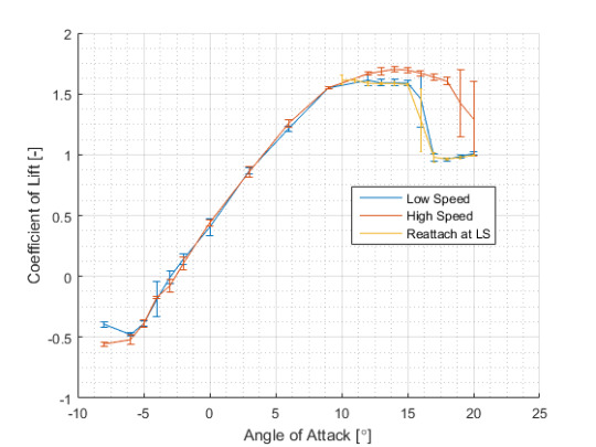
Averages of all Infinite Airfoil Testing Data with Standard Deviations

So, we finished all the infinite airfoil testing last week. And while some of our data looks great, there’s a whole lot of it that is really weird. 

Looking at the standard deviations in our data, above, there are two major trends:

The pressure data generally had a much smaller standard deviation than the data from the wake rake. Naturally, that makes sense because we gathered pressure data from the airfoil for a whole 3 weeks, while the rake was only used during the last two. On top of that, the rake position changed from week 2 to 3, so any differences from that would have an effect on the standard deviation.

In general, the standard deviation increased significantly for angles of attack greater than 15°. From previous testing and research, we know that the NACA 4412 should stall somewhere around 15° for the Reynolds numbers we tested. It’s possible that the turbulent effects surrounding this phenomenon could have effected our data. Though, since we are taking time-averaged data over several seconds, it really shouldn’t.

It seems like we should take a look at how the different testing conditions affected the data, or if there are some other systematic error sources at work here.

Extra Note: Though the high speed tests should have a lower skin friction drag coefficient than the low speed tests, they most certainly should not be negative. There is clearly something going wrong there. But the calculations are the same as the other tests, so it might be a data problem.

[timothylo-blog]

On Tuesday, I found a paper (Models of Lift and Drag Coefficients of Stalled and Unstalled Airfoils in Wind Turbines and Wind Tunnels), in which I found this figure. The lower weight plots show lift and drag coefficients for an infinite aspect ratio airfoil (otherwise known as an infinite airfoil), while the heavier weight show the same for an aspect ratio of 9.04.

As discussed earlier, our airfoil actually isn’t infinite, but we’re attempting to model it as such. So our values should fall somewhere in between the two plots above. For the lift coefficient, our data showed a stall point near that of the finite aspect ratio and a maximum lift value near that of the infinite aspect ratio. Again, this corroborates that our calculations so far are correct.

The interesting part comes in when we compare drag coefficients. At whatever angle of attack the lift coefficient sharply decreases due to stall, the drag coefficient begins to rapidly increase. In both the infinite AR and 9.04 AR plots, remains below 0.1 until the airfoil stalls. After that, the infinite AR shoots up to 0.4 at 20° angle of attack and the 9.04 AR rises to about 0.3. Beyond 20° angle of attack, both airfoils experience maximum drag around 90°, with the infinite airfoil nearly reaching 2.0.

This pattern of having a drag coefficient below 0.1 until the stall point and sharply increasing thereafter is seen quite clearly in each of our data sets. Just before separation at 15° angle of attack all three of our test cases experience a drag coefficient of approximately 0.1. In our limited post stall testing (from  16-20°) we see that the drag coefficient increases to approximately 0.35. This value lies directly between the two drag coefficients found in the NASA report above.

So in the end, it actually appears that our drag coefficients are quite reasonable for the angles of attack we measured at. In future testing it could be interesting to continue investigating these post stall regimes at various Reynolds numbers.

[timothylo-blog]

AIn order to obtain lift and drag coefficients, we discretely integrated the pressure data over the surface of the airfoil. The airfoil was divided into an upper and lower surface, defined from the leading to trailing edge. The first picture shows the locations of each panel of these surfaces and the port located on that panel. We ran into a little issue with this geometry because the first pressure port is located directly on the leading edge. Instead of including this data only as part of the upper surface, we decided to add one smaller panel to both the lower and upper surfaces that used this pressure reading. From there on, the green points align with the ports from the lab manual pictured in an earlier post. The final green point on the trailing edge actually doesn’t represent a pressure port.

Using the builtin Matlab function for numerical integration using the trapezoid rule, we found the normal and axial pressure force along the upper and lower surfaces. Then, it was only a matter of algebra and trigonometry to find the total lift and drag over the airfoil. We took that and non-dimensionalized by the dynamic pressure of the tunnel and the chord length to find the lift and drag coefficients above. Unfortunately, a pesky lost minus sign led us to believe that our drag coefficient was near 0.9 for several days. Even after fixing that mistake, our drag coefficient still skyrocketed well above expected values at higher angles of attack.

For almost a week, we were baffled by this problem. The mathematical analysis behind finding the drag coefficient is extremely closely tied to that for finding the lift coefficient. And our lift coefficient actually came out very close to theory. Based on data from the very extensive airfoil testing conducted by Abbott and Doenhoff in 1945, we expected the airfoil to stall somewhere around 12-15° angle of attack, depending on Reynolds number. Our lift coefficient shows the characteristic “drop-off” of stall around 16° and a maximum lift that matches Abbott and Doenhoff’s 1.6. With such a well regarded reference to corroborate our lift coefficients, we could not figure out how our numbers for drag were so absurdly high.

[timothylo-blog]

After collecting pressure data from the twenty ports, we non-dimensionalized the data and plotted as function of percent chord length. 

We split up the duties of calculating three different pressure coefficients. The analytical pressure for inviscid flow over an infinite wing (not plotted above) was found using potential flow theory.The experimental value (plotted in blue, above) was found by dividing our pressure values by the dynamic pressure of the tunnel. Finally, the numerical, inviscid solution (plotted in red, above) was found using XFoil.

We can note two major differences between the two pressure coefficients:

One of the values at x/c = 0.1 is consistently incorrect. The previous groups reported that there was bad port, and Dr. Doig corroborated that there may be an issue, but that we couldn’t do anything about it for the time being. 

At higher angles of attack (passing 15°), our experimental upper surface values diverge from inviscid theory. This, along with the lift coefficient data that we later found, indicates flow separation around 15° angle of attack. Since XFoil doesn’t analyze the viscous effects that cause separation, its values don’t reflect the changes seen in the real world tests.