#WeirdData

[timothylo-blog]

Breakdown of Low-Speed Tests

Since we wanted to have most of our infinite airfoil testing to be at a Reynolds number we could replicate and compare to the upcoming finite airfoil tests, we have a lot more data to look at here. Unfortunately, we also experimented with different angle of attack sweeps, making it difficult to compare all of the data at once. 

Though most of the tests follow the same trend in the Lift-Drag polar, there are a few oddities:

Two of the reattachment tests showed significant deviation from the rest of the data, while the third did not. The weird thing here is that we expected all of them to show a difference from the tests with ascending angle of attack. I really don’t know why, but the third test’s drag coefficient actually does correlate well with the other two test. The only significant difference occurs in the lift coefficient plot where it deviates from the other two tests, and oddly is even farther away from the increasing angle of attack tests.

Just like the reattachment tests, there was one normal test that was just weird.  For clarity, I added little triangles to this plot. In all three plots, this test almost exactly followed the odd reattachment test for a majority of the tested angles of attack. I went in and checked the numbers to make sure there wasn’t something going wrong with the variables, but it all checked out and the two problem tests were actually different (very slightly). 

The very last normal test, labeled “LS 13~20 3,” had a few odd data points near 15° (expected stall). This test saw a little increase in both lift and drag in this region, but was otherwise normal.

I honestly have no explanations for the first two bullet there. I first made these plots on Friday and have since mulled it over, but I can’t figure it out.

The last point though, we have a well recorded source of error. During the last two tests listed in the legend, we conducted a little bit of flow visualization with smoke. We wanted to take a look at how flow was behaving around the airfoil, and also the rake. The results of that are a whole nother post, but it’s possible that having one of our group members standing directly in front of the tunnel inlet affected our data.

[timothylo-blog]

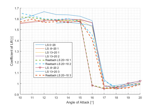
Breakdown of High-Speed Tests

From the standard deviation plots, I noticed that the high speed tests actually had a very reasonable standard deviation throughout the range of angles of attack where we expected separation to occur. The only exceptions were the last two data points, at 19° and 20° angle of attack. To check more into this, I plotted all four of the high speed tests.

From the Lift-Drag polar, we can see that there are two distinct groupings. After checking back to see when each test was run, I found that the two solid line plots were taken before the wake rake was installed and the two dashed line plots were taken afterwards. 

It seems like the presence of the rake is having some sort of influence on our high speed data at higher angles of attack. From the lift coefficient plot, we can see that the characteristic drop off after the airfoil stalls is not present in the tests that included the rake. Instead, the plots begin a slow, linear decline from 16�� to 20° angle of attack. Oddly, the drag coefficient shows that the very first test we conducted is the one that diverges from the group. I’m not entirely sure how to explain that.

The fact that the deviation from previous tests only occurred at high angles of attack during the high speed tests implies that the cause might be dependent on a viscous or blockage effect. The high speed tests were conducted at a higher Reynolds number than the rest of our testing, and were limited in number because they would be impossible to recreate on the finite wings. This higher Reynolds number decreases the influence of viscous effects. I guess that that means it also increases the influence of the pressure effects. 

Blockage, of course, is a pressure effect. Not only is the rake itself most definitely a blunt body, but as the airfoil’s angle of attack is increased it also becomes more like a blunt body than a streamlined one. Due to the proximity of the rake to the trailing edge of the airfoil, it could be possible that the flow reacts to its presence in a way that changes the pressure measured on the airfoil. 

Though it’s not strong, the fact that the purple plot, which was taken with rake moved to the side of the tunnel, is closer to the no-rake tests than the yellow plot, which was taken with the rake in the center. Since our airfoil’s pressure ports are located on the center 20% of the span, it would make sense that this hypothetical phenomenon would be most prominent when the rake is directly behind the ports (i.e.: in the center of the tunnel). 

The increased angle of attack also positions more of the ports along the airfoil’s upper surface such that the normal component is closer to the freestream direction. This increases how much the pressure ports “notice” the presence of the rake downstream, which might explain why the effect only became evident at high angles of attack.

[timothylo-blog]

AIn order to obtain lift and drag coefficients, we discretely integrated the pressure data over the surface of the airfoil. The airfoil was divided into an upper and lower surface, defined from the leading to trailing edge. The first picture shows the locations of each panel of these surfaces and the port located on that panel. We ran into a little issue with this geometry because the first pressure port is located directly on the leading edge. Instead of including this data only as part of the upper surface, we decided to add one smaller panel to both the lower and upper surfaces that used this pressure reading. From there on, the green points align with the ports from the lab manual pictured in an earlier post. The final green point on the trailing edge actually doesn’t represent a pressure port.

Using the builtin Matlab function for numerical integration using the trapezoid rule, we found the normal and axial pressure force along the upper and lower surfaces. Then, it was only a matter of algebra and trigonometry to find the total lift and drag over the airfoil. We took that and non-dimensionalized by the dynamic pressure of the tunnel and the chord length to find the lift and drag coefficients above. Unfortunately, a pesky lost minus sign led us to believe that our drag coefficient was near 0.9 for several days. Even after fixing that mistake, our drag coefficient still skyrocketed well above expected values at higher angles of attack.

For almost a week, we were baffled by this problem. The mathematical analysis behind finding the drag coefficient is extremely closely tied to that for finding the lift coefficient. And our lift coefficient actually came out very close to theory. Based on data from the very extensive airfoil testing conducted by Abbott and Doenhoff in 1945, we expected the airfoil to stall somewhere around 12-15° angle of attack, depending on Reynolds number. Our lift coefficient shows the characteristic “drop-off” of stall around 16° and a maximum lift that matches Abbott and Doenhoff’s 1.6. With such a well regarded reference to corroborate our lift coefficients, we could not figure out how our numbers for drag were so absurdly high.

[timothylo-blog]

Plot of pressure coefficients from the first and second data sets combined.

After considering the possible problems with our first data set, we decided to rerun the experiment with the same sampling parameters. Our reasoning was twofold:

If there really was an unsteady effect, changing our sampling rate might better capture the behavior, but would prevent us from forming any correlations with our first data set. This would force us to run even more tests, or settle for a weaker correlation.

Running the same parameters would let us use our first set of data to form a larger sample size, with which we could analyze the time-averaged behavior with a greater confidence.

With Dr. Doig’s warning in mind, we chose to rotate the cylinder from 90º to 180º instead of 0º to 90º. This was an attempt to balance out any differences between the ports if such a difference existed. In the plot, there is a small but noticeable difference between values for angles that were part of both data sets (90º to 360º).

As with the first set of data, the plots exhibited behaviors similar to what we expected. It is difficult to see, but the sharp changes at 90º and 270º were no more extreme than in the first data set. This suggests that whatever phenomenon occurred in the first test was less prominent or even non-existent in the second. Between this and the consistent difference between readings from each test, there could be enough data to suggest a discrepancy between the ports. We’ll have to look more into this over the weekend.

[timothylo-blog]

Plot of pressure coefficients from the first data set.

This was the first plot we generated in the lab after running the experiment at low and high speeds. In many ways, the trends follow expectations:

Every case follows the inviscid plot fairly close until ~60° above the leading edge.

From there, each case plateaued a constant pressure coefficient around some portion of the leeward side of the cylinder, before following the inviscid plot again.

However, we noticed that all of the experimental plots experience a sharp spike at 90°, 180°, and 270°. We initially considered that his might be caused by a difference between each port’s calibration, since there were measurement overlaps at these angles. We checked with Dr. Doig, who suggested that such a problem had occurred earlier, but that each port was checked for blockages. Of course, he also suggested that we shouldn’t necessarily trust that the ports were all the same.