vishisegal - Tumblr blog

vishisegal · 5 years ago

Text

Predicting whether a person is a Regular Smoker or not using the best Decision Tree from the generated Random Forest

As a part of Assignment for Course: Machine Learning Tools

Steps Involved:

Get the Research Data

Identify the Explanatory Variables: Both Categorical and Quantitative

Load the Dataset

Clean the dataset (remove NAs)

Split dataset in 60:40 ratio, 60% for training model and 40% for testing model

Check Accuracy of the Tree with a defined node.

Check whether other trees are required or not?

Define number of Random Trees in Forest = 25

Plot accuracy of each of them

If the accuracy of other trees is similar to the one we got initially, other trees are not really helpful.

Results Explanation:

2745 records were used for training the model

1830 records were used for testing the model

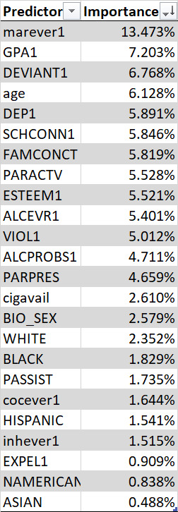
Importance of Explanatory Variables as per the Prediction Model:

Working Code:

import matplotlib.pylab as plt import numpy as np import pandas as pd import sklearn.metrics # Feature Importance from sklearn.ensemble import ExtraTreesClassifier from sklearn.model_selection import train_test_split # Load the dataset AH_data = pd.read_csv('C:\\Users\\M1049673\\Documents\\PythonPractice\\Coursera\\ML\\Datatree_addhealth.csv') AH_data.replace('?', np.nan, inplace=True) data_clean = AH_data.dropna() print('Datatype Information:\n',data_clean.dtypes) print('\nBasic Data related information:\n',data_clean.describe()) # Split into training and testing sets predictors = data_clean[['BIO_SEX','HISPANIC','WHITE','BLACK','NAMERICAN','ASIAN','age', 'ALCEVR1','ALCPROBS1','marever1','cocever1','inhever1','cigavail','DEP1','ESTEEM1','VIOL1', 'PASSIST','DEVIANT1','SCHCONN1','GPA1','EXPEL1','FAMCONCT','PARACTV','PARPRES']] targets = data_clean.TREG1 pred_train, pred_test, tar_train, tar_test = train_test_split(predictors, targets, test_size=.4) print('\nShape of Prediction Train:',pred_train.shape) print('Shape of Prediction Test:',pred_test.shape) print('Shape of Target Train:',tar_train.shape) print('Shape of Target Test:',tar_test.shape) # Build model on training data from sklearn.ensemble import RandomForestClassifier classifier = RandomForestClassifier(n_estimators=25) classifier = classifier.fit(pred_train, tar_train) predictions = classifier.predict(pred_test) print('\nConfusion Matrix:\n',sklearn.metrics.confusion_matrix(tar_test, predictions)) print('Accuracy Score:',sklearn.metrics.accuracy_score(tar_test, predictions)) # fit an Extra Trees model to the data model = ExtraTreesClassifier() model.fit(pred_train, tar_train) # display the relative importance of each attribute print('\nFeatures Importance:',model.feature_importances_) """ Running a different number of trees and see the effect of that on the accuracy of the prediction """ trees = range(25) accuracy = np.zeros(25) for idx in range(len(trees)): classifier = RandomForestClassifier(n_estimators=idx + 1) classifier = classifier.fit(pred_train, tar_train) predictions = classifier.predict(pred_test) accuracy[idx] = sklearn.metrics.accuracy_score(tar_test, predictions) plt.cla() plt.plot(trees, accuracy) plt.show()

Output:

Datatype Information: BIO_SEX float64 HISPANIC float64 WHITE float64 BLACK float64 NAMERICAN float64 ASIAN float64 age float64 TREG1 float64 ALCEVR1 float64 ALCPROBS1 int64 marever1 int64 cocever1 int64 inhever1 int64 cigavail float64 DEP1 float64 ESTEEM1 float64 VIOL1 float64 PASSIST int64 DEVIANT1 float64 SCHCONN1 float64 GPA1 float64 EXPEL1 float64 FAMCONCT float64 PARACTV float64 PARPRES float64 dtype: object

Basic Data related information: BIO_SEX HISPANIC ... PARACTV PARPRES count 4575.000000 4575.000000 ... 4575.000000 4575.000000 mean 1.521093 0.111038 ... 6.290710 13.398033 std 0.499609 0.314214 ... 3.360219 2.085837 min 1.000000 0.000000 ... 0.000000 3.000000 25% 1.000000 0.000000 ... 4.000000 12.000000 50% 2.000000 0.000000 ... 6.000000 14.000000 75% 2.000000 0.000000 ... 9.000000 15.000000 max 2.000000 1.000000 ... 18.000000 15.000000

[8 rows x 25 columns]

Shape of Prediction Train: (2745, 24) Shape of Prediction Test: (1830, 24) Shape of Target Train: (2745,) Shape of Target Test: (1830,)

Confusion Matrix: [[1441 78] [ 190 121]] Accuracy Score: 0.853551912568306

Features Importance: [0.02578917 0.0154114 0.02351627 0.01829161 0.00837805 0.00488314 0.06128191 0.05400669 0.04710931 0.13473079 0.01644478 0.01515276 0.02609708 0.05890997 0.05520846 0.05011535 0.0173519 0.06768484 0.05846291 0.07203345 0.00908774 0.05818886 0.05527677 0.04658681]

0 notes

vishisegal · 7 years ago

Text

ANOVA, Chi-Square Test and correlation coefficient on Automobile data that includes a moderator.

As a part of Assignment for Course: Data Analysis Tools

Lets go through our list of objectives first below:

Identify if variation in Price of car varies according to Body Style and if this variation is further dependent on the Manufacture (i.e. Explanatory Variable-’Body Style’; Response Variable-’Price’; Moderator-’Make Honda and Audi’)

Identify how Body Style varies with Drive Wheel and if this variation is dependent on the Manufacturer (i.e. Explanatory Variable-’Body Style’; Response Variable-’Drive Wheel’; Moderator-’Make Toyota and Mazda’)

Identify if Car Price is related to Horsepower and if this relation is dependent on the choice of Manufacturer (i.e. Explanatory Variable-’Horsepower’; Response Variable-’Price’; Moderator-’Make Toyota and Volvo’)

For better understanding, I would be sharing the result snapshots and code below in 3 parts according to the objectives mentioned above.

*Code for three objectives is present towards the end of this post.

Objective 1: Identify if variation in Price of car varies according to Body Style and if this variation is further dependent on the Manufacture

Steps:

Little data cleaning: data type corrections, remove records with missing data

Observe Price means and Price deviations for total population by Body-Style

Conduct ANOVA on total population: to see overall relation between Body Style and Price

Conduct post hoc Tukey test: to gauge dependence for each combination of Body Style on Price.

Conduct ANOVA separately for Honda cars and Audi cars: to see if relation between Body Style and Price varies with moderator variable like Honda / Audi

Conduct post hoc Tukey test separately for Honda cars and Audi cars : to gauge dependence for each combination of Body Style on Price for each Honda and Audi cars data set.

Result screen-shots and inferences for this objective:

Price means for total population by Body-style showing informations like which type of body-style is more expensive than the other body-style, e.g. convertibles are far more expensive than hatchbacks

Price deviations for total population by Body-style showing information like which category of body-style has more fluctuations than the others, e.g. different hardtops cars price difference is a lot more than different hatchbacks prices.

ANOVA for total population - Low p-value indicating, there is significant relationship between Body-styles and Price

Post hoc Tukey test further showing which body-styles vs body-styles have significant impact on price, e.g. we can confidentially say convertible’s price is higher than hatchbacks (basically, all group1 and group2 are related where reject = True)

ANOVA and post hoc Tukey test below for Audi Cars: Since p-value is high we can easily say that price variation is NOT dependent on body-style for Audi Cars, hence Make of a is a significant Moderator variable

ANOVA and post hoc Tukey test below for Honda Cars: Since p-value is lower than 0.5 we can easily say that price variation is dependent on body-style for Honda Cars, and from Tuckey Test we can further conclude that this relation holds true for hatchback and sedans only for Honda cars. For other combination of body types, price is independent of body-styles.

Objective 2: Identify how Body Style varies with Drive Wheel and if this variation is dependent on the Manufacturer

Steps:

Observe counts of different Drive Wheel categories by Body-Styles - to get an idea of the sample size of each drive wheel type per body-style.

Observe percentage of each category of Drive Wheel by Body-Styles - to get an idea of proportion of each drive wheel per body style.

Conduct Chi square test on total population: to see overall relation between Body Style and Price.

Conduct same steps 1-3 as above for Toyota cars.

Conduct same steps 1-3 as above for Mazda cars.

Plotted graphs showing variation of 4 wheel drive on Price: for full population, for Toyota Population and for Mazda population.

Plotted graphs showing variation of front wheel drive on Price: for full population, for Toyota Population and for Mazda population.

Plotted graphs showing variation of rear wheel drive on Price: for full population, for Toyota Population and for Mazda population.

Result screen-shots and inferences for this objective:

Counts of different Drive Wheel categories by Body-Styles: Shows that majority of the cars are Front Wheel Drive, then Rear Wheel Drive and the number of 4 wheel drive cars are very less in our sample.

Percentage of each category of Drive Wheel by Body-Styles: Indicates information like the proportion of Rear Wheel Drives to Front Wheel Drives is similar for Convertible and Hardtops.

Chi square test on total population: The p value is ~0.0005, indicating there is a significant relationship between Body-Styles and Drive-Wheels.

Same steps as above for Toyota Cars below: As we can see, this time, p-value (~0.007) is higher than 0.003 and hence we can conclude that this relation doesn't hold good for the Toyota cars. i.e. Make/Manufacturer has a moderating effect.

Same steps as above for Mazda Cars below: As we can see, this time, p-value (~0.97) is higher and hence we can conclude that this relation doesn't hold good for the Mazda cars. i.e. Make/Manufacturer has a moderating effect.

Now, lets take a look at graphical comparison of 4 wheel drive category for total population, Toyota and Mazda and as we can see, the pattern is different for Toyota and total population. No graph for Mazda, as Mazda doesn't have a vehicle in four wheel drive segment as per the sample data.

Similarly, for front wheel drive the pattern of Toyota and Mazda is different from Total population.

Similarly, for rear wheel drive the pattern of Toyota and Mazda is different from Total population.

Objective 3: Identify if Car Price is related to Horsepower and if this relation is dependent on the choice of Manufacturer

Steps:

Conduct Pearson correlation test on whole population: Explanatory variable as Horsepower and Response Variable as Price.

Visualize

Conduct Pearson correlation test on Toyota cars: Explanatory variable as Horsepower and Response Variable as Price.

Visualize

Conduct Pearson correlation test on Volvo Cars: Explanatory variable as Horsepower and Response Variable as Price.

Visualize

Result screen-shots and inferences for this objective:

Visualization of Horsepower and Price using scatter-plot and regression plot: We can establish by looking at the plots below that there is a positive relationship between the horsepower and price.

We can further confirm the same by looking at the below Pearson co-efficient values, r value close towards +1 and p is very small

Visualization of Horsepower and Price for Toyota cars using scatter-plot and regression plot: We can establish by looking at the plots below that there is a positive relationship between the horsepower and price for Toyota, which is in line with our overall population.

We can further acknowledge the same by looking at the below Pearson co-efficient values, r value close towards +1 and p is very small

Visualization of Horsepower and Price for Volvo cars using scatter-plot and regression plot: We can establish by looking at the plots below that there is a very scattered almost neutral relationship between the horsepower and price for Volvo, which is in contradiction to over relationship establishment for the overall cars population.

From below values, we can see that there is a weak positive relation based on slightly positive r value, but the high p value clearly indicates, that there is NEUTRAL or NO relationship between horsepower and Price for the Volvo cars, which is in contradiction to over relationship establishment for the overall cars population.

Hence, it is safe to conclude, that variable Manufacture has a significant moderating impact on the relationship between Horsepower and Price.

Now the geek stuff (code):

# Objective = To conduct ANOVA (Audi and Honda), Chi Square(Toyota and Mazda) and # Pearson Correlation (Toyota and Volvo) tests on an automobiles data # set with moderator Variable as Manufacturer/Make import pandas import numpy import matplotlib.pyplot import scipy.stats import seaborn import statsmodels.formula.api as smf import statsmodels.stats.multicomp as multi # Some basic data cleaning steps df = pandas.read_csv('CarTrendData.csv') df.columns = ['Symboling', 'NormalisedLosses', 'Make', 'FuelType', 'Aspiration', 'Numofdoors', 'BodyStyle', 'DriveWheels', 'EngineLocation', 'WheelBase', 'Length', 'Width', 'Height', 'CurbWeight', 'EngineType', 'NumofCylinders', 'EngineSize', 'FuelSystem', 'Bore', 'Stroke', 'CompressionRatio', 'HorsePower', 'PeakRPM', 'CityMPG', 'HighwayMPG', 'Price'] df['Price'].replace('?', numpy.NaN, inplace=True) df['HorsePower'].replace('?', numpy.NaN, inplace=True) df['Price'] = df['Price'].astype('float64') df['HorsePower'] = df['HorsePower'].astype('float64') df = df.dropna() # ANOVA - Explanatory Variable = 'BodyStyle', Response Variable = 'Price' and # Moderator = 'Make= Audi or Honda' dfPriceMean = df[['BodyStyle', 'Price']].groupby(df['BodyStyle']).mean() dfPriceStd = df[['BodyStyle', 'Price']].groupby(df['BodyStyle']).std() print('\nPrice Means by BodyStyle:\n' + str(dfPriceMean)) print('\n\nPrice Deviations by BodyStyle:\n' + str(dfPriceStd)) model = smf.ols(formula='Price ~ C(BodyStyle)', data=df).fit() print(model.summary()) mc = multi.MultiComparison(df['Price'], df['BodyStyle']) result = mc.tukeyhsd() print(result.summary()) # Quick Pivot to get a holistic idea print(str(df.pivot_table(index='Make', columns='BodyStyle', values='Price', aggfunc=numpy.count_nonzero, fill_value=0))) # df[df['Make'].isin(['audi', 'honda'])].to_csv('BaseData.csv') # Another way of writing same thing # df.query('Make in ("audi","honda")').to_csv('BaseData.csv') sub1 = df.query('Make in ("audi")') sub2 = df.query('Make in ("honda")') print('\nANOVA with moderator as Audi') model = smf.ols(formula='Price ~ C(BodyStyle)', data=sub1).fit() print(model.summary()) mc = multi.MultiComparison(sub1['Price'], sub1['BodyStyle']) result = mc.tukeyhsd() print(result.summary()) print('\nANOVA with moderator as Honda') model = smf.ols(formula='Price ~ C(BodyStyle)', data=sub2).fit() print(model.summary()) mc = multi.MultiComparison(sub2['Price'], sub2['BodyStyle']) result = mc.tukeyhsd() print(result.summary()) print('\nConclusion - ' '\n1. Overall car population price is significantly dependent on BodyStyle' '\n2. Price of Audi cars has no relation with BodyStyle as its P-Value came higher than acceptable' '\n3. Honda cars Price has dependency for BodyStyles belonging to Hatchbacks and Sedans. ' 'For other body styles of Honda cars, Price has no relation with BodyStyle') # Chi square - Explanatory Variable = 'BodyStyle', Response Variable = 'DriveWheel', Moderator = 'Make' # Pivot Code to get counts ctl = df.pivot_table(values='Price', index='BodyStyle', columns='DriveWheels', aggfunc=numpy.size, fill_value=0) print('\nPivot Method \n' + str(ctl)) # column Percentages colsum = ctl.sum(axis=0) colpct = round(ctl / colsum, 2) print('\nColumn Percentages\n' + str(colpct)) # Chi square computation chi = scipy.stats.chi2_contingency(ctl) print('\nChi Values :' + str(chi)) # Observing impact of moderator sub1 = df.query('Make in ("toyota")') ctl1 = sub1.pivot_table(values='Price', index='BodyStyle', columns='DriveWheels', aggfunc=numpy.count_nonzero, fill_value=0) print(ctl1) # column Percentages colsum = ctl1.sum(axis=0) colpct = round(ctl1 / colsum, 2) print('\nColumn Percentages\n' + str(colpct)) # Chi square computation chi = scipy.stats.chi2_contingency(ctl1) print('\nChi Values :' + str(chi)) sub2 = df.query('Make in ("mazda")') ctl2 = sub2.pivot_table(values='Price', index='BodyStyle', columns='DriveWheels', aggfunc=numpy.count_nonzero, fill_value=0) print(ctl2) # column Percentages colsum = ctl2.sum(axis=0) colpct = round(ctl2 / colsum, 2) print('\nColumn Percentages\n' + str(colpct)) # Chi square computation chi = scipy.stats.chi2_contingency(ctl2) print('\nChi Values :' + str(chi)) # Charts for comparing ctl['BodyStyle'] = ctl.index ctl1['BodyStyle'] = ctl1.index ctl2['BodyStyle'] = ctl2.index seaborn.pointplot(x='BodyStyle', y='4wd', kind='point', color='green', data=ctl) seaborn.pointplot(x='BodyStyle', y='4wd', kind='point', color='blue', data=ctl1) # seaborn.pointplot(x='BodyStyle', y='4wd', kind='point', color='red', data=ctl2) matplotlib.pyplot.legend(labels=['Total 4wd', 'Toyota 4wd', 'Mazda 4wd']) # , color=['#00639c','#1F04FF','#bb3f3f']) ax = matplotlib.pyplot.gca() leg = ax.get_legend() leg.legendHandles[0].set_color('green') leg.legendHandles[1].set_color('blue') leg.legendHandles[2].set_color('red') matplotlib.pyplot.show() seaborn.pointplot(x='BodyStyle', y='fwd', kind='point', color='green', data=ctl) seaborn.pointplot(x='BodyStyle', y='fwd', kind='point', color='blue', data=ctl1) seaborn.pointplot(x='BodyStyle', y='fwd', kind='point', color='red', data=ctl2) matplotlib.pyplot.legend(labels=['Total fwd', 'Toyota fwd', 'Mazda fwd']) # , color=['#00639c','#1F04FF','#bb3f3f']) ax = matplotlib.pyplot.gca() leg = ax.get_legend() leg.legendHandles[0].set_color('green') leg.legendHandles[1].set_color('blue') leg.legendHandles[2].set_color('red') matplotlib.pyplot.show() seaborn.pointplot(x='BodyStyle', y='rwd', kind='point', color='green', data=ctl) seaborn.pointplot(x='BodyStyle', y='rwd', kind='point', color='blue', data=ctl1) seaborn.pointplot(x='BodyStyle', y='rwd', kind='point', color='red', data=ctl2) matplotlib.pyplot.legend(labels=['Total rwd', 'Toyota rwd', 'Mazda rwd']) # , color=['#00639c','#1F04FF','#bb3f3f']) ax = matplotlib.pyplot.gca() leg = ax.get_legend() leg.legendHandles[0].set_color('green') leg.legendHandles[1].set_color('blue') leg.legendHandles[2].set_color('red') matplotlib.pyplot.show() # Pearson Correlation - Explanatory Variable = 'HorsePower', Response Variable = 'Price', Moderator = 'Make' # ScatterPlot plotting for HorsePower and Price matplotlib.pyplot.show(seaborn.scatterplot(x='HorsePower', y='Price', data=df)) matplotlib.pyplot.show(seaborn.regplot(x='HorsePower', y='Price', data=df)) # Displaying rValue = scipy.stats.pearsonr(df['HorsePower'], df['Price']) print('r coefficient Value for relation between HorsePower and Price is ' + str(rValue[0])) print('P Value for relation between HorsePower and Price is ' + str(rValue[1])) print('r2 Value for relation between HorsePower and Price is ' + str(rValue[0] * rValue[0])) # Understanding impact of moderator sub2 = df.query('Make in ("volvo")') # ScatterPlot plotting for HorsePower and Price matplotlib.pyplot.show(seaborn.scatterplot(x='HorsePower', y='Price', data=sub1)) matplotlib.pyplot.show(seaborn.regplot(x='HorsePower', y='Price', data=sub1)) # Displaying rValue = scipy.stats.pearsonr(sub1['HorsePower'], sub1['Price']) print('Toyota - r coefficient Value for relation between HorsePower and Price is ' + str(rValue[0])) print('Toyota - P Value for relation between HorsePower and Price is ' + str(rValue[1])) print('Toyota - r2 Value for relation between HorsePower and Price is ' + str(rValue[0] * rValue[0])) # ScatterPlot plotting for HorsePower and Price matplotlib.pyplot.show(seaborn.scatterplot(x='HorsePower', y='Price', data=sub2)) matplotlib.pyplot.show(seaborn.regplot(x='HorsePower', y='Price', data=sub2)) # Displaying rValue = scipy.stats.pearsonr(sub2['HorsePower'], sub2['Price']) print('Volvo - r coefficient Value for relation between HorsePower and Price is ' + str(rValue[0])) print('Volvo - P Value for relation between HorsePower and Price is ' + str(rValue[1])) print('Volvo - r2 Value for relation between HorsePower and Price is ' + str(rValue[0] * rValue[0]))

#coursera #python #pycharm

0 notes

vishisegal · 7 years ago

Text

Identification of impact of Automobile’s HorsePower and Mileage on Price using Pearson Coefficient

As a part of Assignment for Course: Data Analysis Tools

As title suggests, we will first find relation between Horse Power and Price.

Steps Followed for Horsepower and Price:

Plotted Scatter-plot for Horsepower and Price

Plotted Regression plot for Horsepower and Price: The positive slope confirms that there is a positive relation between Horsepower and Price

Calculated r coefficient value (0.81) and corresponding p value (1.985 e-47), which further confirms that there is a strong relation between Horsepower and Price

Calculated r-square value (0.657), which indicates that ~65% variability is predictable

Screen-shots for Horsepower and Price:

Steps Followed for Highway-MPG and Price:

Plotted Scatter-plot for Highway-MPG and Price

Plotted Regression plot for Highway-MPG and Price: The negative slope confirms that there is a negative relation between Highway-MPG and Price

Then calculated r coefficient value (-0.706) and corresponding p value (3.773 e-31), which further confirms that there is a strong relation between Highway-MPG and Price

Calculated r-square value (0.498), which indicates that ~50% variability is predictable

Screen-shots for Highway-MPG and Price:

Code:

# To establish relation between Horsepower & Price and relation between Mileage and Price import scipy.stats import seaborn import matplotlib.pyplot import pandas import numpy df = pandas.read_csv('CarTrendData.csv') df.columns = ['Symboling', 'Normalised-Losses', 'Make', 'Fuel-Type', 'Aspiration', 'Num-of-doors', 'Body-Style', 'Drive-Wheels', 'Engine-Location', 'Wheel-Base', 'Length', 'Width', 'Height', 'Curb-Weight', 'Engine-Type', 'Num-of-Cylinders', 'Engine-Size', 'Fuel-System', 'Bore', 'Stroke', 'Compression-Ratio', 'HorsePower', 'Peak-RPM', 'City-MPG', 'Highway-MPG', 'Price'] # Little Data Cleaning df['Price'].replace('?', numpy.NaN, inplace=True) df.dropna(subset=['Price'], axis=0, inplace=True) df['Price'] = df['Price'].astype('float64') df['HorsePower'].replace('?', numpy.NaN, inplace=True) df.dropna(subset=['HorsePower'], axis=0, inplace=True) df['HorsePower'] = df['HorsePower'].astype('float64') df['Highway-MPG'].astype('float64') # ScatterPlot plotting for HorsePower and Price matplotlib.pyplot.show(seaborn.scatterplot(x='HorsePower', y='Price', data=df)) matplotlib.pyplot.show(seaborn.regplot(x='HorsePower', y='Price', data=df)) # Displaying rValue = scipy.stats.pearsonr(df['HorsePower'], df['Price']) print("r coefficient Value for relation between HorsePower and Price is " + str(rValue[0])) print("P Value for relation between HorsePower and Price is " + str(rValue[1])) print("r2 Value for relation between HorsePower and Price is " + str(rValue[0]*rValue[0])) # ScatterPlot plotting for Highway-Mileage and Price matplotlib.pyplot.show(seaborn.scatterplot(x='Highway-MPG', y='Price', data=df)) matplotlib.pyplot.show(seaborn.regplot(x='Highway-MPG', y='Price', data=df)) # Displaying rValue = scipy.stats.pearsonr(df['Highway-MPG'], df['Price']) print("\nr coefficient Value for relation between Highway-MPG and Price is " + str(rValue[0])) print("P Value for relation between Highway-MPG and Price is " + str(rValue[1])) print("r2 Value for relation between Highway-MPG and Price is " + str(rValue[0]*rValue[0])) df.to_csv('A.csv')

#coursera #pycharm #python

0 notes

vishisegal · 7 years ago

Text

Objective: Relation between car Body Style and Drive Wheel

As a part of Assignment for Course: Data Analysis Tools

Here we are going to identify the trend between 4 wheel drive, front wheel drive and rear wheel drive against different body styles like Sedan, Hatchback etc. using Chi Square test.

i.e. Observing relation between 2 categories

Here Body Style has 5 levels and Drive Wheel Types has 3 levels.

Steps:

Loaded car data in dataFrame

Created Pivot (similar to crosstab), for BodyStyles as Index and DriveWheels as Columns with Values as Count of DriveWheels per BodyStyle

Converted to Percentage format for making this information more relevant

Calculated Chi square values using Seaborn library, the high value of F value obtained and low value of p shows that dependency exists

For further analysis, used Seaborn’s pointplot function and matplotlib library for presenting the trend. Added legends with additional set of code for usage of Seaborn with MatplotLib

Conducted post hoc test for selected combinations

-Pivot table screen-shot

-Pivot’s percentage (with roundoff to 2 decimals) screen-shot

-Chi square values screen-shot (showing high F Value and low p-value)

-Seaborn pointplot for independent category (all levels) and dependent category (all levels)

* This plot gives us ideas like:

Sedans and hatchbacks are mostly Front Wheel Drive and rarely 4 wheel drive.

Convertibles and Hardtops are mostly Real Wheel Drive.

Presence of 4 wheel drives are less in all categories.

Post Hoc Test Conclusions for selected combinations:

- Since the p-value can be rounded off to 0.003 which is in acceptable range, we can conclude that majority of the Hatchbacks are Front Wheel Drives and majority of the Hardtops are Rear Wheel Drive

- Since the p-value is high, we accept the null hypothesis concluding that there is no relationship between sedan or wagon being front wheel drive or a rear wheel drive

Code:

import numpy import pandas import scipy.stats import seaborn import matplotlib.pyplot # Loading car data to data frame df = pandas.read_csv('CarTrendData.csv', header=None) headers = ['Symboling', 'NormalisedLosses', 'Make', 'FuelType', 'Aspiration', 'Numofdoors', 'BodyStyle', 'DriveWheels', 'EngineLocation', 'WheelBase', 'Length', 'Width', 'Height', 'CurbWeight', 'EngineType', 'NumofCylinders', 'EngineSize', 'FuelSystem', 'Bore', 'Stroke', 'CompressionRatio', 'HorsePower', 'PeakRPM', 'CityMPG', 'HighwayMPG', 'Price'] df.columns = headers df.to_csv('CarTrendData_Base.csv') # To study how BodyStyles of car are related to Drive Wheel Category # Pivot Code to get counts ctl = df.pivot_table(values='Price', index='BodyStyle', columns='DriveWheels', aggfunc=numpy.size, fill_value=0) print('\nPivot Method \n' + str(ctl)) # column percentages colsum = ctl.sum(axis=0) colpct = round(ctl / colsum, 2) print('\nPercentage \n' + str(colpct)) # chi-square print('\n\nchi-square value, p value, expected counts') cs1 = scipy.stats.chi2_contingency(ctl) print(cs1) ctl['BodyStyle'] = ctl.index seaborn.pointplot(x='BodyStyle', y='4wd', data=ctl, color='green', label='4wd') seaborn.pointplot(x='BodyStyle', y='fwd', data=ctl, color='#1F04FF', label='fwd') seaborn.pointplot(x='BodyStyle', y='rwd', data=ctl, color='#bb3f3f', label='rwd') matplotlib.pyplot.legend(labels=['4wd', 'fwd', 'rwd']) # , color=['#00639c','#1F04FF','#bb3f3f']) ax = matplotlib.pyplot.gca() leg = ax.get_legend() leg.legendHandles[0].set_color('green') leg.legendHandles[1].set_color('#1F04FF') leg.legendHandles[2].set_color('#bb3f3f') matplotlib.pyplot.ylabel('Rear Wheel Drive') matplotlib.pyplot.xlabel('Body Style') matplotlib.pyplot.show() # post hoc test for selected combinations print('\nFor relation between HardTop & Hatchback on Rear wheel drive and Front Wheel Drive') ctl = df.pivot_table(values='Price', index='BodyStyle', columns='DriveWheels', aggfunc=numpy.size, fill_value=0) ctl = ctl[['fwd', 'rwd']].query('BodyStyle == ["hatchback","hardtop"]') print('Pivot Method \n' + str(ctl)) # column percentages colsum = ctl.sum(axis=0) colpct = round(ctl / colsum, 2) print('\nPercentage \n' + str(colpct)) # chi-square print('\n\nchi-square value, p value, expected counts') cs1 = scipy.stats.chi2_contingency(ctl) print(cs1) print('\nFor relation between Wagon & Sedan on Rear wheel drive and Front Wheel Drive') ctl = df.pivot_table(values='Price', index='BodyStyle', columns='DriveWheels', aggfunc=numpy.size, fill_value=0) ctl = ctl[['fwd', 'rwd']].query('BodyStyle == ["wagon","sedan"]') print('Pivot Method \n' + str(ctl)) # column percentages colsum = ctl.sum(axis=0) colpct = round(ctl / colsum, 2) print('\nPercentage \n' + str(colpct)) # chi-square print('\n\nchi-square value, p value, expected counts') cs1 = scipy.stats.chi2_contingency(ctl) print(cs1)

#coursera #python #pycharm

0 notes