deba1407

[deba1407]

KMeans Clustering Assignment

Import the modules

from pandas import Series, DataFrame import pandas as pd import numpy as np import matplotlib.pylab as plt from sklearn.model_selection import train_test_split from sklearn import preprocessing from sklearn.cluster import KMeans

Load the dataset

data = pd.read_csv("C:\Users\guy3404\OneDrive - MDLZ\Documents\Cross Functional Learning\AI COP\Coursera\machine_learning_data_analysis\Datasets\tree_addhealth.csv")

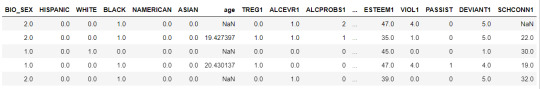
data.head()

upper-case all DataFrame column names

data.columns = map(str.upper, data.columns)

Data Management

data_clean = data.dropna() data_clean.head()

subset clustering variables

cluster=data_clean[['ALCEVR1','MAREVER1','ALCPROBS1','DEVIANT1','VIOL1', 'DEP1','ESTEEM1','SCHCONN1','PARACTV', 'PARPRES','FAMCONCT']] cluster.describe()

standardize clustering variables to have mean=0 and sd=1

clustervar=cluster.copy() clustervar['ALCEVR1']=preprocessing.scale(clustervar['ALCEVR1'].astype('float64')) clustervar['ALCPROBS1']=preprocessing.scale(clustervar['ALCPROBS1'].astype('float64')) clustervar['MAREVER1']=preprocessing.scale(clustervar['MAREVER1'].astype('float64')) clustervar['DEP1']=preprocessing.scale(clustervar['DEP1'].astype('float64')) clustervar['ESTEEM1']=preprocessing.scale(clustervar['ESTEEM1'].astype('float64')) clustervar['VIOL1']=preprocessing.scale(clustervar['VIOL1'].astype('float64')) clustervar['DEVIANT1']=preprocessing.scale(clustervar['DEVIANT1'].astype('float64')) clustervar['FAMCONCT']=preprocessing.scale(clustervar['FAMCONCT'].astype('float64')) clustervar['SCHCONN1']=preprocessing.scale(clustervar['SCHCONN1'].astype('float64')) clustervar['PARACTV']=preprocessing.scale(clustervar['PARACTV'].astype('float64')) clustervar['PARPRES']=preprocessing.scale(clustervar['PARPRES'].astype('float64'))

split data into train and test sets

clus_train, clus_test = train_test_split(clustervar, test_size=.3, random_state=123)

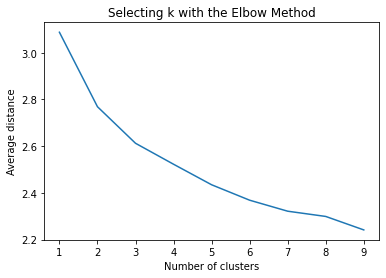
k-means cluster analysis for 1-9 clusters

from scipy.spatial.distance import cdist clusters=range(1,10) meandist=[]

for k in clusters: model=KMeans(n_clusters=k) model.fit(clus_train) clusassign=model.predict(clus_train) meandist.append(sum(np.min(cdist(clus_train, model.cluster_centers_, 'euclidean'), axis=1)) / clus_train.shape[0])

""" Plot average distance from observations from the cluster centroid to use the Elbow Method to identify number of clusters to choose """ plt.plot(clusters, meandist) plt.xlabel('Number of clusters') plt.ylabel('Average distance') plt.title('Selecting k with the Elbow Method')

Interpret 3 cluster solution

model3=KMeans(n_clusters=3) model3.fit(clus_train) clusassign=model3.predict(clus_train)

plot clusters

from sklearn.decomposition import PCA pca_2 = PCA(2) plot_columns = pca_2.fit_transform(clus_train) plt.scatter(x=plot_columns[:,0], y=plot_columns[:,1], c=model3.labels_,) plt.xlabel('Canonical variable 1') plt.ylabel('Canonical variable 2') plt.title('Scatterplot of Canonical Variables for 3 Clusters') plt.show()

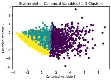
The datapoints of the 2 clusters in the left are less spread out but have more overlaps. The cluster to the right is more distinct but has more spread in the data points

""" BEGIN multiple steps to merge cluster assignment with clustering variables to examine cluster variable means by cluster """

create a unique identifier variable from the index for the

cluster training data to merge with the cluster assignment variable

clus_train.reset_index(level=0, inplace=True)

create a list that has the new index variable

cluslist=list(clus_train['index'])

create a list of cluster assignments

labels=list(model3.labels_)

combine index variable list with cluster assignment list into a dictionary

newlist=dict(zip(cluslist, labels)) newlist

convert newlist dictionary to a dataframe

newclus=DataFrame.from_dict(newlist, orient='index') newclus

rename the cluster assignment column

newclus.columns = ['cluster']

now do the same for the cluster assignment variable

create a unique identifier variable from the index for the

cluster assignment dataframe

to merge with cluster training data

newclus.reset_index(level=0, inplace=True)

merge the cluster assignment dataframe with the cluster training variable dataframe

by the index variable

merged_train=pd.merge(clus_train, newclus, on='index') merged_train.head(n=100)

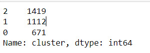
cluster frequencies

merged_train.cluster.value_counts()

""" END multiple steps to merge cluster assignment with clustering variables to examine cluster variable means by cluster """

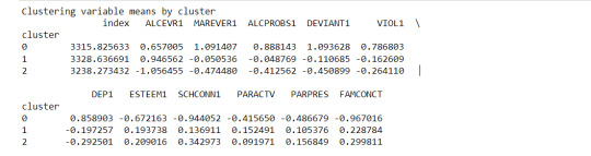
FINALLY calculate clustering variable means by cluster

clustergrp = merged_train.groupby('cluster').mean() print ("Clustering variable means by cluster") print(clustergrp)

validate clusters in training data by examining cluster differences in GPA using ANOVA

first have to merge GPA with clustering variables and cluster assignment data

gpa_data=data_clean['GPA1']

split GPA data into train and test sets

gpa_train, gpa_test = train_test_split(gpa_data, test_size=.3, random_state=123) gpa_train1=pd.DataFrame(gpa_train) gpa_train1.reset_index(level=0, inplace=True) merged_train_all=pd.merge(gpa_train1, merged_train, on='index') sub1 = merged_train_all[['GPA1', 'cluster']].dropna()

Print statistical summary by cluster

import statsmodels.formula.api as smf import statsmodels.stats.multicomp as multi

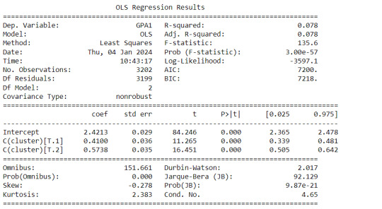
gpamod = smf.ols(formula='GPA1 ~ C(cluster)', data=sub1).fit() print (gpamod.summary())

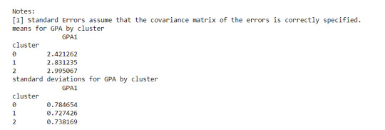
print ('means for GPA by cluster') m1= sub1.groupby('cluster').mean() print (m1)

print ('standard deviations for GPA by cluster') m2= sub1.groupby('cluster').std() print (m2)

Interpretation

The clustering average summary shows Cluster 0 has higher alcohol and marijuana problems, shows higher deviant and violent behavior, suffers from depression, has low self esteem,school connectedness, paraental and family connectedness. On the contrary, Cluster 2 shows the lowest alcohol and marijuana problems, lowest deviant & violent behavior,depression, and higher self esteem,school connectedness, paraental and family connectedness. Further, when validated against GPA score, we observe Cluster 0 shows the lowest average GPA and CLuster 2 has the highest average GPA which aligns with the summary statistics interpretation.

[deba1407]

Running Lasso Regression Analysis

Import Libraries

from pandas import Series, DataFrame import pandas as pd import numpy as np import os import matplotlib.pylab as plt from sklearn.model_selection import train_test_split from sklearn.linear_model import LassoLarsCV

Load the dataset

data = pd.read_csv("C:\Users\guy3404\OneDrive - MDLZ\Documents\Cross Functional Learning\AI COP\Coursera\machine_learning_data_analysis\Datasets\tree_addhealth.csv")

Getting information aboubt the dataset

data.info()

upper-case all DataFrame column names

data.columns = map(str.upper, data.columns)

Total size of data

len(data)

We observe some of the columns of the dataset contains null values . We need to drop them

Drop Null values

data_clean = data.dropna()

Data management

recode1 = {1:1, 2:0} data_clean['MALE']= data_clean['BIO_SEX'].map(recode1)

Length of dataset after dropping null values

len(data_clean)

Split into training and testing sets

select predictor variables and target variable as separate data sets

predvar= data_clean[['MALE','HISPANIC','WHITE','BLACK','NAMERICAN','ASIAN', 'AGE','ALCEVR1','ALCPROBS1','MAREVER1','COCEVER1','INHEVER1','CIGAVAIL','DEP1', 'ESTEEM1','VIOL1','PASSIST','DEVIANT1','GPA1','EXPEL1','FAMCONCT','PARACTV', 'PARPRES']]

target = data_clean.SCHCONN1

standardize predictors to have mean=0 and sd=1

predictors=predvar.copy() from sklearn import preprocessing predictors['MALE']=preprocessing.scale(predictors['MALE'].astype('float64')) predictors['HISPANIC']=preprocessing.scale(predictors['HISPANIC'].astype('float64')) predictors['WHITE']=preprocessing.scale(predictors['WHITE'].astype('float64')) predictors['NAMERICAN']=preprocessing.scale(predictors['NAMERICAN'].astype('float64')) predictors['ASIAN']=preprocessing.scale(predictors['ASIAN'].astype('float64')) predictors['AGE']=preprocessing.scale(predictors['AGE'].astype('float64')) predictors['ALCEVR1']=preprocessing.scale(predictors['ALCEVR1'].astype('float64')) predictors['ALCPROBS1']=preprocessing.scale(predictors['ALCPROBS1'].astype('float64')) predictors['MAREVER1']=preprocessing.scale(predictors['MAREVER1'].astype('float64')) predictors['COCEVER1']=preprocessing.scale(predictors['COCEVER1'].astype('float64')) predictors['INHEVER1']=preprocessing.scale(predictors['INHEVER1'].astype('float64')) predictors['CIGAVAIL']=preprocessing.scale(predictors['CIGAVAIL'].astype('float64')) predictors['DEP1']=preprocessing.scale(predictors['DEP1'].astype('float64')) predictors['ESTEEM1']=preprocessing.scale(predictors['ESTEEM1'].astype('float64')) predictors['VIOL1']=preprocessing.scale(predictors['VIOL1'].astype('float64')) predictors['PASSIST']=preprocessing.scale(predictors['PASSIST'].astype('float64')) predictors['DEVIANT1']=preprocessing.scale(predictors['DEVIANT1'].astype('float64')) predictors['GPA1']=preprocessing.scale(predictors['GPA1'].astype('float64')) predictors['EXPEL1']=preprocessing.scale(predictors['EXPEL1'].astype('float64')) predictors['FAMCONCT']=preprocessing.scale(predictors['FAMCONCT'].astype('float64')) predictors['PARACTV']=preprocessing.scale(predictors['PARACTV'].astype('float64')) predictors['PARPRES']=preprocessing.scale(predictors['PARPRES'].astype('float64'))

split data into train and test sets

pred_train, pred_test, tar_train, tar_test = train_test_split(predictors, target, test_size=.3, random_state=123)

specify the lasso regression model

model=LassoLarsCV(cv=10, precompute=False).fit(pred_train,tar_train)

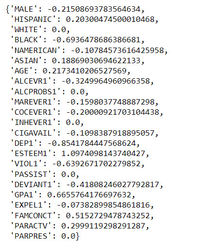
print variable names and regression coefficients

dict(zip(predictors.columns, model.coef_))

plot coefficient progression

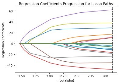
m_log_alphas = -np.log10(model.alphas_) ax = plt.gca() plt.plot(m_log_alphas, model.coef_path_.T) plt.axvline(-np.log10(model.alpha_), linestyle='--', color='k', label='alpha CV') plt.ylabel('Regression Coefficients') plt.xlabel('-log(alpha)') plt.title('Regression Coefficients Progression for Lasso Paths')

MSE from training and test data

from sklearn.metrics import mean_squared_error train_error = mean_squared_error(tar_train, model.predict(pred_train)) test_error = mean_squared_error(tar_test, model.predict(pred_test)) print ('training data MSE') print(train_error) print ('test data MSE') print(test_error)

R-square from training and test data

rsquared_train=model.score(pred_train,tar_train) rsquared_test=model.score(pred_test,tar_test) print ('training data R-square') print(rsquared_train) print ('test data R-square') print(rsquared_test)

Summary

The study used lasso regression to figure out which factors affect how connected adolescents feel to school. They had 23 variables, including things like age, substance use, and family-related factors. The data was split into a training set (70%) and a test set (30%). The model found 18 key variables that together explained 33.4% of the variation in school connectedness. Self-esteem, depression, violent behavior, and GPA were the strongest influencers. Positive factors included older age, Hispanic/Asian ethnicity, family connectedness, and parental involvement. Negative factors included being mal, Black/Native American, substance use, deviant behavior, and expulsion history. The R square and MSE values of both train and test datasets are very close, indicating a lower variance in the model results.

[deba1407]

Running a Random Forest

from pandas import Series, DataFrame import pandas as pd import numpy as np import os import matplotlib.pylab as plt from sklearn.model_selection import train_test_split from sklearn.tree import DecisionTreeClassifier from sklearn.metrics import classification_report import sklearn.metrics # Feature Importance from sklearn import datasets from sklearn.ensemble import ExtraTreesClassifier

Load the dataset

data = pd.read_csv("C:\Users\guy3404\OneDrive - MDLZ\Documents\Cross Functional Learning\AI COP\Coursera\machine_learning_data_analysis\Datasets\tree_addhealth.csv")

data.head()

Getting information aboubt the dataset

data.info()

Total size of data

len(data)

We observe some of the columns of the dataset contains null values . We need to drop them

Drop null values from dataset

data_clean = data.dropna()

data_clean.dtypes

data_clean.describe()

Length of dataset after dropping null values

len(data_clean)

Split into training and testing sets

predictors = data_clean[['BIO_SEX','HISPANIC','WHITE','BLACK','NAMERICAN','ASIAN','age', 'ALCEVR1','ALCPROBS1','marever1','cocever1','inhever1','cigavail','DEP1','ESTEEM1','VIOL1', 'PASSIST','DEVIANT1','SCHCONN1','GPA1','EXPEL1','FAMCONCT','PARACTV','PARPRES']]

targets = data_clean.TREG1

pred_train, pred_test, tar_train, tar_test = train_test_split(predictors, targets, test_size=.4)

pred_train.shape pred_test.shape tar_train.shape tar_test.shape

Build model on training data

from sklearn.ensemble import RandomForestClassifier

classifier=RandomForestClassifier(n_estimators=25) classifier=classifier.fit(pred_train,tar_train)

predict using random forest classifier on test data

predictions=classifier.predict(pred_test)

Print confusion matrix and accuracy score

sklearn.metrics.confusion_matrix(tar_test,predictions)

sklearn.metrics.accuracy_score(tar_test, predictions)

fit an Extra Trees model to the data

model = ExtraTreesClassifier() model.fit(pred_train,tar_train)

Get feature importances

feature_importances = model.feature_importances_

Create a Series with feature importances and corresponding feature names

feature_importance_series = pd.Series(feature_importances, index=pred_train.columns)

Sort features based on importance

sorted_feature_importance = feature_importance_series.sort_values(ascending=False)

Plot the feature importances

plt.figure(figsize=(10, 6)) sorted_feature_importance.plot(kind='barh') plt.title('Feature Importance') plt.xlabel('Importance Score') plt.show()

#Running different number of trees and see the effect of that on the accuracy of the prediction

trees=range(25) accuracy=np.zeros(25)

for idx in range(len(trees)): classifier=RandomForestClassifier(n_estimators=idx + 1) classifier=classifier.fit(pred_train,tar_train) predictions=classifier.predict(pred_test) accuracy[idx]=sklearn.metrics.accuracy_score(tar_test, predictions)

plt.cla() plt.plot(trees, accuracy)

Random forest analysis was performed to evaluate the importance of series of variables in predicting whether a person is a regular smoker or not. We observed that out of all features, marijuana use has the highest feature importance, followed by deviance and GPA. The random model could predict with an accuracy score of 85%.