flyingbaloonblog

[flyingbaloonblog]

Coursera Regression Modeling in Practice - Assignment week 4

Results

the selected response variable (lifeexpectancy from gapminder dataset) is a quantitative variable, therefore i binned that variable such that ‘1’ corresponded to the 3rd quantile and above while ‘0’ corresponded to less than the 3rd quantile, accordingly i designed the label of the new (binary) response variable as ‘life_score’ from the quantitative ‘lifeexpectancy’.

Running logistic regressions for the 4 explanatory variables i found the following evidence:

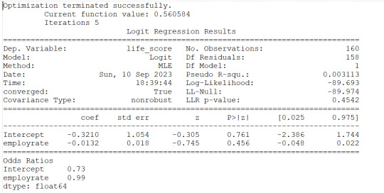
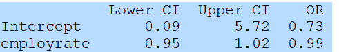
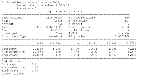
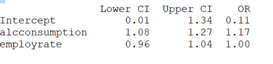
1) employrate is not associated to the response variable (life_score) since the pvalue is 0.456 and altough the OR=0.99 is slightly less than 1, the 95% Confidence Interval contains 1 therefore no probability that the employrate would impact the life_score

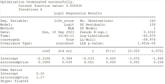
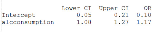
2) alcconsumption is instead significantly associated to the response variable based on the pvalue<0.0001 and the OR=1.17 with the 95%CI of 1.08 to 1.27 would indicate that people with large alcconsumption would have between 1.08 and 1.27 more probability to live longer than the 3rd quantile.

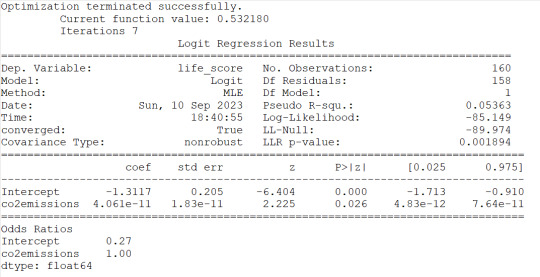
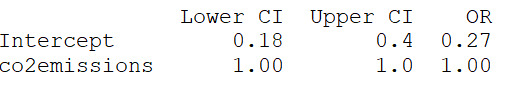
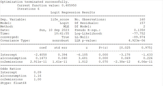
3) co2emissions seems to be associated to the response variable because of the pvof 0.026 but the OR of 1 would indicate that there is no significant impact on probability for life expectancy

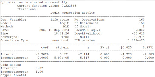
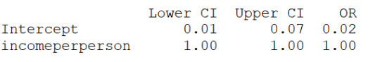
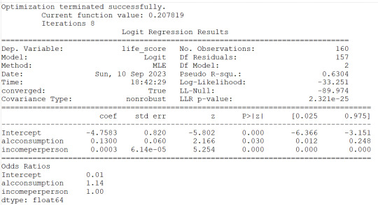
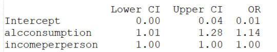
4)incomeperperson show same reesults as for co2emissions therefore same conclusions can be drawn.

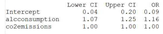
I then checked for confounding and found no evidence of it when running regression with alcconsumption and the other 3 explanatory variables as shown (in the results) by the unchanged level of significance of the alcconsumption. I can state then that the alcconsumprion is significantly associated to the life expenctancy (coeff=0.1585, pvalue<0.0001, OR=1.17, 95%IC=1.08 - 1.27 after adjusting for the other explanatory variables. Therefore people with larger alcconsumption would have 1.08 to 1.27 better propbability to live at/above the 3rd quantitle.

This result is partially supporting my hypothesis (since 1 out of 4 explanatory variables have an association with the response variable) but it is also counterintuitive to the expectation of alcohol consumption favouring longer life expectancy. Overlall this week results confirms the past week (week 3) outcome of a basically misspecified model which is missing some other important explanatory variables.

Details and code are following.

Code

import numpy

import pandas

import statsmodels.api as sm

import statsmodels.formula.api as smf

data=pandas.read_csv('gapminder.csv',low_memory=False)

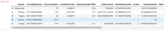
data.head()

data['incomeperperson']=pandas.to_numeric(data['incomeperperson'],errors='coerce')

data['alcconsumption']=pandas.to_numeric(data['alcconsumption'],errors='coerce')

data['co2emissions']=pandas.to_numeric(data['co2emissions'],errors='coerce')

data['employrate']=pandas.to_numeric(data['employrate'],errors='coerce')

data['lifeexpectancy']=pandas.to_numeric(data['lifeexpectancy'],errors='coerce')

sub1=data[['incomeperperson','alcconsumption','co2emissions', 'employrate','lifeexpectancy']].dropna()

#binning lifeexpectancy to be 1 at and above 3rd quantile and moving to the new variable 'life_score'

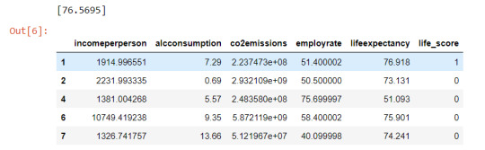
v=numpy.quantile(sub1['lifeexpectancy'],[0.75])

print(v)

sub1['life_score']=['1' if x >= v else '0' for x in sub1['lifeexpectancy']]

sub1['life_score']=pandas.to_numeric(sub1['life_score'],errors='coerce')

sub1.head()

#logistic regression for employment rate

lreg1=smf.logit(formula='life_score ~ employrate', data=sub1).fit()

print(lreg1.summary())

print('Odds Ratios')

print (round(numpy.exp(lreg1.params),2))

#odd ratios with 95% conf interval

params=lreg1.params

conf=lreg1.conf_int()

conf['OR']=params

conf.columns=['Lower CI', 'Upper CI', 'OR']

print(round(numpy.exp(conf),2))

#logistic regression for alcohol consumption

lreg1=smf.logit(formula='life_score ~ alcconsumption', data=sub1).fit()

print(lreg1.summary())

print('Odds Ratios')

print (round(numpy.exp(lreg1.params),2))

#odd ratios with 95% conf interval

params=lreg1.params

conf=lreg1.conf_int()

conf['OR']=params

conf.columns=['Lower CI', 'Upper CI', 'OR']

print(round(numpy.exp(conf),2))

#logistic regression for CO2 emissions

lreg1=smf.logit(formula='life_score ~ co2emissions', data=sub1).fit()

print(lreg1.summary())

print('Odds Ratios')

print (round(numpy.exp(lreg1.params),2))

#odd ratios with 95% conf interval

params=lreg1.params

conf=lreg1.conf_int()

conf['OR']=params

conf.columns=['Lower CI', 'Upper CI', 'OR']

print(round(numpy.exp(conf),2))

#logistic regression for incomeperperson

lreg1=smf.logit(formula='life_score ~ incomeperperson', data=sub1).fit()

print(lreg1.summary())

print('Odds Ratios')

print (round(numpy.exp(lreg1.params),2))

#odd ratios with 95% conf interval

params=lreg1.params

conf=lreg1.conf_int()

conf['OR']=params

conf.columns=['Lower CI', 'Upper CI', 'OR']

print(round(numpy.exp(conf),2))

#check for confounding - adding c02emissions to alcohol consumption

lreg1=smf.logit(formula='life_score ~ alcconsumption+co2emissions', data=sub1).fit()

print(lreg1.summary())

print('Odds Ratios')

print (round(numpy.exp(lreg1.params),2))

#odd ratios with 95% conf interval

params=lreg1.params

conf=lreg1.conf_int()

conf['OR']=params

conf.columns=['Lower CI', 'Upper CI', 'OR']

print(round(numpy.exp(conf),2))

#check for confounding - adding incomeperperson to alcohol consumption

lreg1=smf.logit(formula='life_score ~ alcconsumption+incomeperperson', data=sub1).fit()

print(lreg1.summary())

print('Odds Ratios')

print (round(numpy.exp(lreg1.params),2))

#odd ratios with 95% conf interval

params=lreg1.params

conf=lreg1.conf_int()

conf['OR']=params

conf.columns=['Lower CI', 'Upper CI', 'OR']

print(round(numpy.exp(conf),2))

#check for confounding - adding employment rate to alcohol consumption

lreg1=smf.logit(formula='life_score ~ alcconsumption+employrate', data=sub1).fit()

print(lreg1.summary())

print('Odds Ratios')

print (round(numpy.exp(lreg1.params),2))

#odd ratios with 95% conf interval

params=lreg1.params

conf=lreg1.conf_int()

conf['OR']=params

conf.columns=['Lower CI', 'Upper CI', 'OR']

print(round(numpy.exp(conf),2))

[flyingbaloonblog]

Coursera. Regression in practice. Assignment Week 3.

Summary of results (more details in the code section)

The multiple regression model results show that only 2 (income per person and employment rate) are significantly associated to the response variable (life expectancy) which would make sense since high value of both explanatory variables would indicate healthy economy and lifestyle and a quality healthcare: The results also show that the other 2 explanatory variables (CO2 emissions and alcohol consumption) are not associated while I was expecting that large values of those 2 explanatory variables were associated to low value of life expectancy.

Numeric results are in the following table

Clearly the results do not fully support my hypothesis but only partially as only 2 of the 4 explanatory variables I considered are significantly associated to the response. The 2 associated variables explain about 55% of the response variability indicating that some other important explanatory variable is missing.

There is no evidence of confounding introduced by the not associated variables as the significant association of the other 2 explanatory variables does not reduce when controlling for the other variables.

The diagnostic plots that were generated (and shown in the Code section) and residuals analysis indicate that the fit of the model is impacted by some curvilinear trend which is not adequately represented by the quadratic term used. The plots also show some large residual especially at the lower values of the explanatory variables and the presence of some outliers with little leverage (therefore not influencing the model quality) and 1 observation with a big leverage which is not an outlier). No evidence that the model could be improved by removing (if possible at all) those outliers/high leverage observations. Also, the percentage of observations with a residual greater than absolute 2.5 sigma is bigger than 1% and the percentage of observations with a residual greater than absolute 2 sigma is bigger than 5% indicating that the model fit is poor.

The final conclusion is that the model is partially mis-specified as other important explanatory variables are missing.    

More details in the comments in the Code section below.

CODE and Comments

import numpy

import pandas

import matplotlib.pyplot as plt

import statsmodels.api as sm

import statsmodels.formula.api as smf

import seaborn

pandas.set_option('display.float_format', lambda x:'%.2f'%x)

# loading dataset

data = pandas.read_csv('gapminder.csv')

# convert to numeric format

data['lifeexpectancy'] = pandas.to_numeric(data['lifeexpectancy'], errors='coerce')

data['incomeperperson'] = pandas.to_numeric(data['incomeperperson'], errors='coerce')

data['alcconsumption'] = pandas.to_numeric(data['alcconsumption'], errors='coerce')

data['co2emissions'] = pandas.to_numeric(data['co2emissions'], errors='coerce')

data['employrate'] = pandas.to_numeric(data['employrate'], errors='coerce')

# listwise deletion of missing values

sub1 = data[['lifeexpectancy', 'incomeperperson', 'alcconsumption','co2emissions','employrate']].dropna()

#start screening of explanatory variables (income per person)

# run the 2 scatterplots together to get both linear and second order fit lines

scat1 = seaborn.regplot(x="incomeperperson", y="lifeexpectancy", scatter=True, data=sub1)

scat1 = seaborn.regplot(x="incomeperperson", y="lifeexpectancy", scatter=True, order=2, data=sub1)

plt.xlabel('Income per Person')

plt.ylabel('Life Expectancy')

# comment1: Income per person shows curvilinear trend, will be considering linear and quadratic terms

#continuing screening of explanatory variables (alcohol consumption)

scat1 = seaborn.regplot(x="alcconsumption", y="lifeexpectancy", scatter=True, data=sub1)

scat1 = seaborn.regplot(x="alcconsumption", y="lifeexpectancy", scatter=True, order=2, data=sub1)

plt.xlabel('Alcohol Consumption')

plt.ylabel('Life Expectancy')

# comment2: Alcohol Consumption shows weak curvilinear trend mainly driven by an extreme value, will be considering only linear term

#continuing screening of explanatory variables (CO2 emissions)

scat1 = seaborn.regplot(x="co2emissions", y="lifeexpectancy", scatter=True, data=sub1)

scat1 = seaborn.regplot(x="co2emissions", y="lifeexpectancy", scatter=True, order=2, data=sub1)

plt.xlabel('CO2 emissions')

plt.ylabel('Life Expectancy')

# comment3: CO2 emissions shows weak curvilinear trend mainly driven by an extreme value, will be considering only linear term

#completing screening of explanatory variables (employment rate)

scat1 = seaborn.regplot(x="employrate", y="lifeexpectancy", scatter=True, data=sub1)

scat1 = seaborn.regplot(x="employrate", y="lifeexpectancy", scatter=True, order=2, data=sub1)

plt.xlabel('Employment Rate')

plt.ylabel('Life Expectancy')

# comment4: Employment rate shows strong curvilinear trend, will be considering both linear and quadratic terms

# centering quantitative explanatory Variables for regression analysis

sub1['incomeperperson_c'] = (sub1['incomeperperson'] - sub1['incomeperperson'].mean())

sub1['alcconsumption_c'] = (sub1['alcconsumption'] - sub1['alcconsumption'].mean())

sub1['co2emissions_c'] = (sub1['co2emissions'] - sub1['co2emissions'].mean())

sub1['employrate_c'] = (sub1['employrate'] - sub1['employrate'].mean())

sub1[["incomeperperson_c", "alcconsumption_c",'co2emissions_c','employrate_c']].describe()

# comment5: mean of explanatory variables is zero or very close to zero.

# evaluating regression model with screened explanatory variables

reg3 = smf.ols('lifeexpectancy  ~ incomeperperson_c+ I(incomeperperson_c**2) + alcconsumption_c + co2emissions_c + employrate_c+I(employrate_c**2)', data=sub1).fit()

print (reg3.summary())

#Comment6: Only Incomeperperson (linear and quadratic terms) and employrate (only linear term) qre significantly associated to #the response variable (their Pvalue is ≤ 0.0001 and the 95% Confidence Interval does not contain 0).

# All the explanatory variables explain no more than 55% of all the response variability (early warning that some #additional explanatory variable may be missing)

# Confounding Check. Establishing the baseline

reg3 = smf.ols('lifeexpectancy  ~ incomeperperson_c+I(incomeperperson_c**2) + employrate_c',

               data=sub1).fit()

print (reg3.summary())

#Comment7:The intercept is indicating that when the 2 associated explanatory variables are at their mean value, the #lifeexpectancy is 71.9 years. To be noted that R-squared is not quite high as 70% or greater to be able to state that the #model is well capturing the variation of life expectancy.

# adding alcohol consumption

reg4 = smf.ols('lifeexpectancy  ~ incomeperperson_c+I(incomeperperson_c**2)+ employrate_c + alcconsumption_c',

               data=sub1).fit()

print (reg4.summary())

#Comment8: no evidence of confounding when adding alcohol consumption (main association does not change)

# adding co2 emissions

reg4 = smf.ols('lifeexpectancy  ~ incomeperperson_c + I(incomeperperson_c**2) + employrate_c + co2emissions_c',

               data=sub1).fit()

print (reg4.summary())

#Comment9: no evidence of confounding when adding co2 emissions (main association does not change)

# diagnostic plots for reg3 baseline regression model

#Q-Q plot for normality

fig4=sm.qqplot(reg3.resid, line='r')

#Comment10: Plot shows that residual are not following a normal distribution as they are highly deviating atlow and #high quartiles. This indicates that the regression model is not well specified as curvilinear trend is not well explained by #the quadratic term and/or some additional explanatory variables are missing.

# simple plot of residuals

stdres=pandas.DataFrame(reg3.resid_pearson)

plt.plot(stdres, 'o', ls='None')

l = plt.axhline(y=0, color='r')

plt.ylabel('Standardized Residual')

plt.xlabel('Observation Number')

#Comment11: The plot shows that most of the residuals is within 1 sigma but also that there are more than 1% of the #observations  with residual greater than absolute 2.5sigma and more than 5% of the observations with a residual #greater than absolute 2sigma, also one observation has a residual greater than 3 sigma  (extreme outlier). This #indicates that the model should be Improved and that some important explanatory variable is missing.

# additional regression diagnostic plots --- contribution of incomeperperson

fig2=plt.figure(figsize=(12,8)) fig2 = sm.graphics.plot_regress_exog(reg3,  "incomeperperson_c", fig=fig2)

#Comment12:the upper right plot shows the residual vs income per person with a curvilinear trend and a clear poor fit #at low level of income. It also shows a clear outlier. The lower left plot (partial regression plot) confirms a curvilinear #trend which is not fully explained by the quadratic terms which has been included in the regression model after #controlling for the other explanatory variable.

# additional regression diagnostic plots --- contribution of employment rate

fig2=plt.figure(figsize=(12,8))

fig2 = sm.graphics.plot_regress_exog(reg3,  "employrate_c", fig=fig2)

#Comment13:the upper right plot shows the residual vs employment rate which along with the partial regression plot #does not clearly indicate a non linear trend but they show rather some large residual qfter controlling for the other explanatory variable.

#Leverage plot

fig4=sm.graphics.influence_plot(reg3,size=8)

print(fig4)

#Comment14: plot shows some outliers with small leverage therefore not particularly influencing the model accuracy and 1 observation with large residual but not an outlier.

[flyingbaloonblog]

Assignment2-Coursera-Regression-modeling-in-practice

The following is for the week2 assignment.

Code

import numpy as numpyp

import pandas as pandas

import statsmodels.api

import statsmodels.formula.api as smf

import seaborn

import matplotlib.pyplot as plt

# bug fix for display formats to avoid run time errors

pandas.set_option('display.float_format', lambda x:'%.2f'%x)

#call in data set

data = pandas.read_csv('gapminder.csv')

# convert variables to numeric format using convert_objects function

data['lifeexpectancy'] = pandas.to_numeric(data['lifeexpectancy'], errors='coerce')

data['employrate'] = pandas.to_numeric(data['employrate'], errors='coerce')

sub1=data[['employrate']].dropna() sub1['employrate_c']=(sub1['employrate']-sub1['employrate'].mean()) print(sub1['employrate_c'].mean())

scat1 = seaborn.regplot(x="employrate", y="lifeexpectancy", scatter=True, data=data)

plt.xlabel('employrate')

plt.ylabel('Life Expectancy')

plt.title ('Scatterplot for the Association Between Life Exp. and Employement rate')

print(scat1)

print ("OLS regression model for the association between Life expectancy and employrate")

reg1 = smf.ols('lifeexpectancy ~ employrate', data=data).fit()

print (reg1.summary())

OUTPUT

Mean of quantitative explanatory variables employrate =  58.64

Mean of centered quantitative explanatory variables employrate =  -2.674514791905995e-15

Discussion

The linear regression model shows that the quantitative explanqtory variable employrate is significantly associated with the quantitative response variable lifeexpectancy since the p value is ‹0.0001 therefore the null hypothesis (no association can be rejected). The coefficient of the explanatory variables is also significant (p value ‹0.0001) but negative meaning that the response variable decreases when the explanatory variable increases as also shown by the plot. However, the explanatory variable only explain 11% of the response variable total variability (R-squared=0.106).

[flyingbaloonblog]

Coursera regression modeling in practice.Assignment 1.

Sample.

the datasample for this study reports several socio-economics indicators (like number of people living in urban areas, number of internet user for a given number of people, etc…) for 213 countries. The sample is drawn from databases made available by Gapminder (www.gapminder.com) a non-profits organization supporting sustainable global development.

Procedure

Data has been collected by Gapminder through several International organization sources like, but not limited to, World Health Organization, World bank, International Energy Agency.

Each record of the database used for this study reports data aggregated by Country so that Country is an unique identifier in the considered database. Data is referred to or up to a given year, to “per capita”, to “percentage of population” or to “given number of people”, as applicable.

Measure

The following variables are considered in this study:

Life expectancy (analysis var name: “lifeexpectancy”) is expressed in number of years and it is the average number of years a newborn child would live assuming the mortality rate stays as per the 2011. Data is from Human Mortality and Human Lifetable databases, World population Prospects and Publications and files by hystory prof James C Riley.

Personal income (analysis var name: “incomeperperson”) is the 2010 Gross Domestic Product per capita in constant 2000 US$. Inflation, but not the difference in the cost of living between countries has been considered. Data is from World Bank Work Development Indicator.

Alcohol Consumption (analysis var name:”alcconsumption”) is the 2008 alcohol consumption per adult (age 15+) in liters. Data is from the World Health Organization.

Carbon dioxide emission (analysis var name:”co2emissions”) is the 2006 cumulative CO2 emission (metric tons), total amount of CO2 emission in metric tons since 1751. Data is from the CDIAC (Carbon Dioxide Information Analysis Center).

Employment rate (analysis var name:”employrate”) is the 2007 total employees age 15+ ( %of population). Percentage of total population, age above 15, that has been employeed during the given year. Data is from the International Labour Organization.

The research question is ”there is an association between life expectancy (response variable) and income per person, alcohol consumption, Carbon dioxide emissions and employment rate (the explanatory variables)”?

In addressing the research question the whole original database is split into 2 subsets.

The first subset comprises the 27 countries part of the European Union (as of the 2023, but not considering special territories like Netherlands Antilles) plus USA, Canada, UK, Japan and Australia while the second comprises all the remaining 181 countries of the original database.

In this study, Statistica regression tools are used to verify any association between response and explanatory variables and to build predictive models to evaluate the significancy of the difference (if any) between response variable for the 2subset.