
Don't wanna be here? Send us removal request.
Statistics
We looked inside some of the posts by jkaraszi and here's what we found interesting.
Average Info
Notes Per Post
1
Likes Per Post
1
Reblog Per Post
0
Reply Per Post
0
Time Between Posts
6 days
Number of Posts By Type
Text
8
Last Seen Tumblr Blogs


Fun Fact
Tumblr Inc. is using 66 technologies for its website.
Text
Data Analysis Tools (week4 - Python)
""" Spyder Editor
This is a temporary script file. """
libraries are imported here
import pandas import numpy import seaborn import matplotlib.pyplot as plt import scipy
csv file is loaded here
data = pandas.read_csv('gapminder.csv', low_memory=False)
bug fix for display formats to avoid run time errors
pandas.set_option('display.float_format', lambda x:'%f'%x)
number of observations (rows)
print (len(data))
number of variables (columns)
print (len(data.columns)) # number of variables (columns)
setting variables to numeric
data['incomeperperson'] = pandas.to_numeric(data['incomeperperson'],errors="coerce") data['lifeexpectancy'] = pandas.to_numeric(data['lifeexpectancy'],errors="coerce") data['polityscore'] = pandas.to_numeric(data['polityscore'],errors="coerce")
setting missing data: empty cells, drop not a number values
data.loc['incomeperperson']=data['incomeperperson'].replace(' ', numpy.nan) data.loc['lifeexpectancy']=data['lifeexpectancy'].replace(' ', numpy.nan) data.loc['polityscore']=data['polityscore'].replace(' ', numpy.nan)
make a copy of the original data
sub_data = data.copy()
Polityscore categories creation
def polityscoregrp (row): if row['polityscore'] <= -5: return 1 elif row['polityscore'] <= 0 : return 2 elif row['polityscore'] <= 5: return 3 elif row['polityscore'] > 5: return 4
sub_data['ps_cat'] = sub_data.apply (lambda row: polityscoregrp (row),axis=1) data_clean=sub_data.dropna()
sub1=data_clean[(data_clean['ps_cat']== 1)] sub2=data_clean[(data_clean['ps_cat']== 2)] sub3=data_clean[(data_clean['ps_cat']== 3)] sub4=data_clean[(data_clean['ps_cat']== 4)]
Scatterplot: Q->Q (Incomeperperson->Lifeexpectancy)
scat1 = seaborn.regplot(x="incomeperperson", y="lifeexpectancy", fit_reg=True, data=data_clean) plt.xlabel('Income per person') plt.ylabel('Life expectancy') plt.title('Scatterplot for the Association Between Income Per Person and Life Expectancy') plt.show()
Correlation coefficient Q->Q (Incomeperperson->Lifeexpectancy)
print ('association between Life Expectancy and Income Per Person') print (scipy.stats.pearsonr(data_clean['incomeperperson'], data_clean['lifeexpectancy'])) print (len(data_clean))
Correlation coefficient Q->Q (Incomeperperson->Lifeexpectancy)
print ('association between Life Expectancy and Income Per Person for countries with Autocracy') print (scipy.stats.pearsonr(sub1['incomeperperson'], sub1['lifeexpectancy'])) print (len(sub1))
scat1 = seaborn.regplot(x="incomeperperson", y="lifeexpectancy", fit_reg=True, data=sub1) plt.xlabel('Income per person') plt.ylabel('Life expectancy') plt.title('Scatterplot for the Association Between Income Per Person and Life Expectancy with Autocracy') plt.show()
print ('association between Life Expectancy and Income Per Person for countries with Semi-Autocracy') print (scipy.stats.pearsonr(sub2['incomeperperson'], sub2['lifeexpectancy'])) print (len(sub2))
scat1 = seaborn.regplot(x="incomeperperson", y="lifeexpectancy", fit_reg=True, data=sub2) plt.xlabel('Income per person') plt.ylabel('Life expectancy') plt.title('Scatterplot for the Association Between Income Per Person and Life Expectancy with Semi-Autocracy') plt.show()
print ('association between Life Expectancy and Income Per Person for countries with Semi-Democracy') print (scipy.stats.pearsonr(sub3['incomeperperson'], sub3['lifeexpectancy'])) print (len(sub3))
scat1 = seaborn.regplot(x="incomeperperson", y="lifeexpectancy", fit_reg=True, data=sub3) plt.xlabel('Income per person') plt.ylabel('Life expectancy') plt.title('Scatterplot for the Association Between Income Per Person and Life Expectancy with Semi-Democracy') plt.show()
print ('association between Life Expectancy and Income Per Person for countries with Democracy') print (scipy.stats.pearsonr(sub4['incomeperperson'], sub4['lifeexpectancy'])) print (len(sub4))
scat1 = seaborn.regplot(x="incomeperperson", y="lifeexpectancy", fit_reg=True, data=sub4) plt.xlabel('Income per person') plt.ylabel('Life expectancy') plt.title('Scatterplot for the Association Between Income Per Person and Life Expectancy with Democracy') plt.show()
Background: I used the GapMinder database for my assignment (Testing moderation in the context of correlation). In my assignment I examined the association between Life expectancy (quantitative response) and Income per person (quantitative explanatory) while the Polityscore as moderation (categorical) was tested. As for the Polityscore I have created four categories, four Polityscore group variable (as 1- Autocracy, 2- Semi-Autocracy, 3- Semi-Democracy and 4- Democracy) based on the value of Polityscore (level of country's democratic and free nature).
Result:
Summary: For the Countries with high negative Polityscore (Autocracy), the correlation between Life expectancy and Income per person is 0.36 and the p-value is not significant (0,09).

For the Countries with low negative Polityscore (Semi-Autocracy), the correlation between Life expectancy and Income per person is 0.55 and the p-value is significant (0,004).

For the Countries with low positive (Semi-Democracy), the correlation between Life expectancy and Income per person is 0.51 and the p-value is significant (0,027).

For the Countries with high Polityscore (Democracy), the correlation between Life expectancy and Income per person is 0.63 and the p-value is significant (3.5e-11).

Finally, I can conlude excluding those countries where the polityscores are in the higher negative range (Autocracy) where almost there is no relationship, there is positive association between Life expectancy and Income per person.
For the visualization scatter plots are used for each group of political systems. Estimating a line of best fit within each scatter plot shows the positive association between Life expectancy and Income per person among those countries where the political system is not Autocracy. At those countries the original hypothesis could be confirmed Wealth is Health.
The political system through the level of democracy affects Life expectancy only indirectly through wealth in these countries (Semi-Autocracy, Semi-Democracy, Democracy).
Post hoc tests are not necessary when conducting Pearson correlation.


0 notes
Text
Data Analysis Tools (week3 - Python)
Scatterplot: Q->Q (Incomeperperson->Lifeexpectancy)
scat1 = seaborn.regplot(x="incomeperperson", y="lifeexpectancy", fit_reg=True, data=data) plt.xlabel('Income per person') plt.ylabel('Life expectancy') plt.title('Scatterplot for the Association Between Income Per Person and Life Expectancy') plt.show()
data_clean=data.dropna()
Correlation coefficient Q->Q (Incomeperperson->Lifeexpectancy)
print ('association between Life Expectancy and Income Per Person') print (scipy.stats.pearsonr(data_clean['incomeperperson'], data_clean['lifeexpectancy']))
Background: I used the Gapminder database for my assignment (Pearson Correlation). In my assignment I examined the association between the Life Expectancy (quantitative response variable) and Income Per Person (quantitative explanatory variable).
Result: The correlation coefficient assesses the degree of linear relationship between two variables. The correlation coefficient is approximately 0.61 with a very small p-value (3.078e-17), it tells us the relationship is statistically significant.
The association between Life Expectancy and Income Per Person is positive, but modest at 0.61 (considering linear regression).
For the Correlation Coefficient between Income per person and Life expectancy, the R-squared is 0.37. This suggests that if we know the Income per person, we can explain about 37% of the variability in Life Expectancy.

The scatter plot between these two variables shows a clear relationship/trend between between the Income Per Person and the Life expectancy variables.

0 notes
Text
Data Analysis Tools (week2 - Python)
contingency table of observed counts
ct1=pandas.crosstab(sub2['S2AQ6A_N'], sub2['REGION']) print (ct1)
column percentages
colsum=ct1.sum(axis=0) colpct=ct1/colsum print(colpct)
chi-square
print ('chi-square value, p value, expected counts') cs1= scipy.stats.chi2_contingency(ct1) print (cs1)
set variable types
sub2["REGION"] = sub2["REGION"].astype('category')
new code for setting variables to numeric:
sub2['S2AQ6A_N'] = pandas.to_numeric(sub2['S2AQ6A_N'], errors='coerce')
seaborn.catplot(x="REGION", y="S2AQ6A_N", data=sub2, kind="bar", errorbar=None) plt.xlabel('Region') plt.ylabel('Wine consumption')
1->2
recode1 = {1: 1, 2: 2} sub2['COMP1v2']= sub2['REGION'].map(recode1)
contingency table of observed counts
ct2=pandas.crosstab(sub2['S2AQ6A_N'], sub2['COMP1v2']) print (ct2)
column percentages
colsum=ct2.sum(axis=0) colpct=ct2/colsum print(colpct)
print ('chi-square value, p value, expected counts') cs2= scipy.stats.chi2_contingency(ct2) print (cs2)
1->3
recode2 = {1: 1, 3: 3} sub2['COMP1v3']= sub2['REGION'].map(recode2)
contingency table of observed counts
ct3=pandas.crosstab(sub2['S2AQ6A_N'], sub2['COMP1v3']) print (ct3)
column percentages
colsum=ct3.sum(axis=0) colpct=ct3/colsum print(colpct)
print ('chi-square value, p value, expected counts') cs3= scipy.stats.chi2_contingency(ct3) print (cs3)
1->4
recode3 = {1: 1, 4: 4} sub2['COMP1v4']= sub2['REGION'].map(recode3)
contingency table of observed counts
ct4=pandas.crosstab(sub2['S2AQ6A_N'], sub2['COMP1v4']) print (ct4)
column percentages
colsum=ct4.sum(axis=0) colpct=ct4/colsum print(colpct)
print ('chi-square value, p value, expected counts') cs4= scipy.stats.chi2_contingency(ct4) print (cs4)
2->3
recode4 = {2: 2, 3: 3} sub2['COMP2v3']= sub2['REGION'].map(recode4)
contingency table of observed counts
ct5=pandas.crosstab(sub2['S2AQ6A_N'], sub2['COMP2v3']) print (ct5)
column percentages
colsum=ct5.sum(axis=0) colpct=ct5/colsum print(colpct)
print ('chi-square value, p value, expected counts') cs5= scipy.stats.chi2_contingency(ct5) print (cs5)
2->4
recode5 = {2: 2, 4: 4} sub2['COMP2v4']= sub2['REGION'].map(recode5)
contingency table of observed counts
ct6=pandas.crosstab(sub2['S2AQ6A_N'], sub2['COMP2v4']) print (ct6)
column percentages
colsum=ct6.sum(axis=0) colpct=ct6/colsum print(colpct)
print ('chi-square value, p value, expected counts') cs6= scipy.stats.chi2_contingency(ct6) print (cs6)
3->4
recode6 = {3: 3, 4: 4} sub2['COMP3v4']= sub2['REGION'].map(recode6)
contingency table of observed counts
ct7=pandas.crosstab(sub2['S2AQ6A_N'], sub2['COMP3v4']) print (ct7)
column percentages
colsum=ct7.sum(axis=0) colpct=ct7/colsum print(colpct)
print ('chi-square value, p value, expected counts') cs7= scipy.stats.chi2_contingency(ct7) print (cs7)
Background: I used the NECARC (National Epidemiologic Survey of Drug Use and Health) database for my assignment (Chi-Square Test). In my assignment I examined the association between wine consumption habits (categorical response) and Region (categorical explanatory). Only those observations (male in Early adulthood) who drank at least 1 alcoholic drink in the last 12 months, it means the current Abstainer were excluded in this study. Region: 1. Northeast 2. Midwest 3. South 4. West
Result: Chi-square test of independence revealed there is association between the wine consumption habit and the Region as the null hypothesis saying there is no association could be rejected based on the p value (p value=5.8e-15).

As the explanatory variables have 4levels the chi-square statistic and associated p-value do not provide information why the null hypothesis can be rejected, therefore Post hoc test was required. I need to perform 6 paired comparisons, so the adjusted p value = 0,05/6 = 0,008.


Post hoc comparisons of rates of wine consumption habit by pairs of region revealed in Region1 there is the highest wine consumption rate (50.3%) while the lowest is in Region3 (36.9%). There wine consumption rate is statistically similar among Region2 (41.8%) and Region4 (43.3%) (p value=0.35)

0 notes
Text
Data Analysis Tools (week1 - Python)
#created a new dataframe only with the relevant variables
data21 = data2[['ipp_cat', 'lifeexpectancy']].dropna()
#using ols function for calculating the F-statistic and associated p value
model1 = smf.ols(formula='lifeexpectancy ~ C(ipp_cat)', data=data21) results1 = model1.fit() print (results1.summary())
print ('means for Lifeexpectancy by category of Incomeperperson') m_le= data21.groupby('ipp_cat').mean() print (m_le)
print ('standard deviations for Lifeexpectancy by category of Incomeperperson') sd_le = data21.groupby('ipp_cat').std() print (sd_le)
#Post hoc test for Anova
mc_le = multi.MultiComparison(data21['lifeexpectancy'], data21['ipp_cat']) res_le = mc_le.tukeyhsd() print(res_le.summary())
Hypothesis: The original hypothesis was that life expectancy is mostly a function of people's wealth, which ensures their access to a healthy lifestyle (living environment, nutrition, work-life balance) and health care.
Graphical assessment: The scatter graph does show a clear relationship/trend between strong relationship between the Income Per Person and the Life expectancy variables.
Statistical assessment: Model Interpretation for ANOVA:
For the ANOVA tool I categorized the countries based on the Income per person into 3 categories as low: less than 1k US$ medium: 1k - 10k US$ high: over 10k$
ANOVA tool was used to examine association between the Life expectancy (quantitative response variable) and the Income per person (categorical explanatory variable). The data provides significant evidence (F-statistic: 135.7, p<<0,5) against the null hypothesis (Ho) so I rejected the null hypothesis with accepting the alternate hypothesis (Ha) saying the explanatory (Income per person) and the response variables (Life expectancy) are associated.

Model Interpretation for post hoc ANOVA results:
With rejecting the null hypothesis Post hoc test comparisons were performed for ANOVA. Post hoc test comparisons of mean number (Tukey HSD) of the Life expectancy by Income per person (categories) revealed that those countries where the Income per person is higher the people has higher life expectancy. Differences could be seen between each groups. Higher income means longer Life,


0 notes
Text
Data Management and Visualization (week4 - Python)
#-- coding: utf-8 --
""" Spyder Editor
This is a temporary script file. """
#libraries are imported here
import pandas import numpy import seaborn import matplotlib.pyplot as plt
#csv file is loaded here
data = pandas.read_csv('gapminder.csv', low_memory=False)
#bug fix for display formats to avoid run time errors
pandas.set_option('display.float_format', lambda x:'%f'%x)
#number of observations (rows)
print (len(data))
#number of variables (columns)
print (len(data.columns)) # number of variables (columns)
#setting variables to numeric
data['incomeperperson'] = pandas.to_numeric(data['incomeperperson'],errors="coerce") data['lifeexpectancy'] = pandas.to_numeric(data['lifeexpectancy'],errors="coerce") data['polityscore'] = pandas.to_numeric(data['polityscore'],errors="coerce")
#make a copy of the original data
sub_data = data.copy()
#setting missing data: empty cells, drop not a number values
data.loc['incomeperperson']=data['incomeperperson'].replace(' ', numpy.nan) data.loc['lifeexpectancy']=data['lifeexpectancy'].replace(' ', numpy.nan) data.loc['polityscore']=data['polityscore'].replace(' ', numpy.nan)
#Incomeperperson categories creation
create a list of conditions for incomeperperson
conditions_ipp = [ (data['incomeperperson'] <= 1000), (data['incomeperperson'] > 1000) & (data['incomeperperson'] <= 10000), (data['incomeperperson'] > 10000) & (data['incomeperperson'] <= 50000), (data['incomeperperson'] > 50000) ]
#create a list of the values for incomeperperson
values_ipp = ['less than 1k US$', '1k - 10k US$', '10k-50k US$', 'over 50k US$']
#create a new column and use numpy.select to assign values to it
data['ipp_cat'] = numpy.select(conditions_ipp, values_ipp)
#remove observations where no data available
data2 = data[data['ipp_cat'] != '0']
#Lifeexpectancy categories creation
create a list of conditions for lifeexpectacy
conditions_le = [ (data['lifeexpectancy'] <= 60), (data['lifeexpectancy'] > 60) & (data['lifeexpectancy'] <= 70), (data['lifeexpectancy'] > 70) & (data['lifeexpectancy'] <= 80), (data['lifeexpectancy'] > 80) ]
#create a list of the values for lifeexpectacy
values_le = ['less than 60yr', '60-70yr', '70-80yr', 'over 80yr']
#create a new column and use numpy.select to assign values to it
data['le_cat'] = numpy.select(conditions_le, values_le)
data3 = data[data['le_cat'] != '0']
#Printing out Count and Frequency (Polityscore)
print('Counts for Polityscore') c_ps = data['polityscore'].value_counts(sort=True) print (c_ps)
print('Percentages for Polityscore') p_ps = data['polityscore'].value_counts(sort=True, normalize=True) * 100 print (p_ps)
#Printing out the number of countries where no data was available (Polityscore)
print ('Printing out the number of countries where no data was available (Polityscore):') sub1 = sub_data[pandas.isna(sub_data['polityscore'])] print (len(sub1))
xPrinting out Count and Frequency (Incomeperperson) with Categories
print('Counts for Incomeperperson by categories, Low: < 1000 US$, Medium: < 10000 US$, High: < 50000 US$, Extreme high: > 50000 US$') c_ipp = data2.groupby('ipp_cat').size() print(c_ipp)
print('Percentages for Incomeperson by categories, Low: < 1000 US$, Medium: < 10000 US$, High: < 50000 US$, Extreme high: > 50000 US$') p_ipp = data2.groupby('ipp_cat').size()*100/len(data2) print(p_ipp)
#Printing out the number of countries where no data was available (Incomeperperson)
print ('Printing out the number of countries where no data was available (Incomeperson):') print (len(sub_data)-len(data2))
#Printing out Count and Frequency (Lifeexpectancy) with Categories
print('Counts for Lifeexpectancy by categories, Low: < 60 yr, Medium: < 70 yr, High: < 80 yr, Extreme high: > 80 yr') c_le = data3.groupby('le_cat').size() print(c_le)
print('Percentages for Lifeexpectancy categories, Low: < 60 yr, Medium: < 70 yr, High: < 80 yr, Extreme high: > 80 yr') p_le = data3.groupby('le_cat').size()*100/len(data3) print(p_le)
#Printing out the number of countries where no data was available (Lifeexpectancy)
print ('Printing out the number of countries where no data was available (Lifeexpectancy):') print (len(sub_data)-len(data3))
#Polityscore
print ('describe polityscore') desc_pc = data2['polityscore'].describe() print (desc_pc)
print ('mode of polityscore') mode_ps = data['polityscore'].mode() print (mode_ps)
seaborn.displot(data['polityscore'], kde=True) plt.xlabel('polityscore') plt.show()
#Incomeperperson
print ('describe incomeperperson') desc_ipp = data2['incomeperperson'].describe() print (desc_ipp)
print ('mode of incomeperperson') mode_ipp = data2['incomeperperson'].mode() print (mode_ipp)
print ('median of incomeperperson') median_ipp = data2['incomeperperson'].median() print (median_ipp)
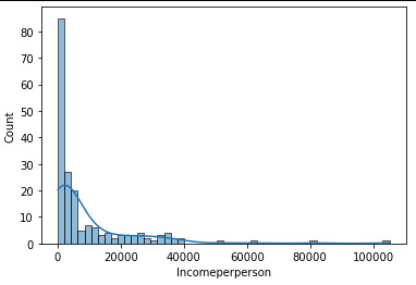
seaborn.histplot(data2['incomeperperson'], bins= 50, kde=True) plt.xlabel('Incomeperperson') plt.show()
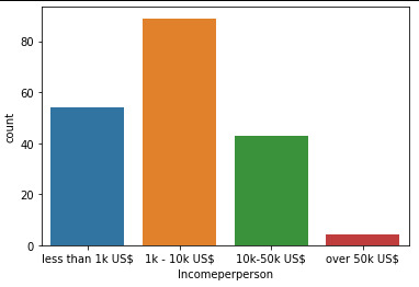
seaborn.countplot(data=data2, x="ipp_cat", order=['less than 1k US$', '1k - 10k US$', '10k-50k US$', 'over 50k US$']) plt.xlabel('Incomeperperson') plt.show()
#Lifeexpectancy
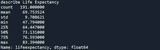
print ('describe Life Expectancy') desc_le = data3['lifeexpectancy'].describe() print (desc_le)
print ('mode of Life Expectancy') mode_le = data2['lifeexpectancy'].mode() print (mode_le)
seaborn.displot(data3['lifeexpectancy'], kde=True) plt.xlabel('Lifeexpectancy') plt.show()
seaborn.countplot(data=data3, x="le_cat", order=['less than 60yr', '60-70yr', '70-80yr', 'over 80yr']) plt.xlabel('Lifeexpectancy') plt.show()
#Scatterplot: Q->Q (Incomeperperson->Lifeexpectancy)
scat1 = seaborn.regplot(x="incomeperperson", y="lifeexpectancy", fit_reg=True, data=data, logx=True) plt.xlabel('Income per person') plt.ylabel('Life expectancy') plt.title('Scatterplot for the Association Between Income Per Person and Life Expectancy') plt.show()
#Scatterplot: Q->Q (Polityscore->Lifeexpectancy)
scat2 = seaborn.regplot(x="polityscore", y="lifeexpectancy", fit_reg=False, data=data) plt.xlabel('Polity score') plt.ylabel('Life expectancy') plt.title('Scatterplot for the Association Between Polity Score and Life Expectancy') plt.show()
SUMMARY:
Three variables selected which are linked to my original research question and hypothesis.
Lifeexpectancy (response)
Polityscore (explanatory)
Incomeperperson (explanatory)
The dataset used: gapminder.csv
Lifeexpectancy (response): This graph is unimodal, with its highest peak at 70 to 75 years old. It seems to be skewed to the left as there are higher frequencies in the higher age ranges.


Polityscore (explanatory): This graph is unimodal, with its highest peak at 10 (full democracy) it shows at most of the observed countries there is full democracy, although at some countries there is autocracy. The graph is skewed to the left as there are higher frequencies in the higher Polity Score ranges.


Incomeperperson (explanatory): This graph is unimodal and skewed to the right. Excluding some countries with extremely high Income per person, most of the countries in the lower income range. Instead of using mean value, the median (2555 US$) is representing better the observed countries.

Hypothesis: The original hypothesis was that life expectancy is mostly a function of people's wealth, which ensures their access to a healthy lifestyle (living environment, nutrition, work-life balance) and health care and the level of democracy affects life expectancy only indirectly through wealth. The scatter graph does not show a clear relationship/trend between the Democracy level and the Life expectancy variables while presents strong relationship between the Income Per Person and the Life expectancy variables. So, the original hypothesis could be confirmed Wealth is Health.


0 notes
Text
Data Management and Visualization (week3 - Python)
# -- coding: utf-8 --
""" Spyder Editor
This is a temporary script file. """
#libraries are imported here
import pandas import numpy
#csv file is loaded here
data = pandas.read_csv('nesarc_pds.csv', low_memory=False)
#bug fix for display formats to avoid run time errors
pandas.set_option('display.float_format', lambda x:'%f'%x)
#print (len(data)) #number of observations (rows)
#print (len(data.columns)) # number of variables (columns)
#setting variables to numeric
data['AGE'] = pandas.to_numeric(data['AGE'],errors="coerce") data['S2AQ6A'] = pandas.to_numeric(data['S2AQ6A'],errors="coerce") data['S2AQ6G'] = pandas.to_numeric(data['S2AQ6G'],errors="coerce") data['S2AQ6H'] = pandas.to_numeric(data['S2AQ6H'],errors="coerce")
#setting missing data: empty cells, drop not a number values or unknown values
data.loc['AGE']=data['AGE'].replace(' ', numpy.nan) data.loc['S2AQ6A']=data['S2AQ6A'].replace(' ', numpy.nan) data['S2AQ6A']=data['S2AQ6A'].replace(9, numpy.nan) data.loc['S2AQ6G']=data['S2AQ6G'].replace(' ', numpy.nan) data.loc['S2AQ6G']=data['S2AQ6G'].replace(99, numpy.nan) data.loc['S2AQ6H']=data['S2AQ6H'].replace(' ', numpy.nan) data.loc['S2AQ6H']=data['S2AQ6H'].replace(9, numpy.nan)
#subset data to young adults only
sub1=data[(data['AGE']>=18) & (data['AGE']<=25)]
#make a copy of subset for the proper management of newly created variables
sub2=sub1.copy()
#recoding values for S2AQ6A into a new variable, Wine_drank
recode1 = {1: 'Drank', 2: 'Not Drunk'} sub2['Wine_drank']= sub2['S2AQ6A'].map(recode1)
#Printing out Count and Frequency (Wine consumption yes/no)
print('counts for Wine consumption') c1 = sub2['Wine_drank'].value_counts(sort=False, dropna=True) print(c1)
print('percentages for Wine consumption') c2 = sub2['Wine_drank'].value_counts(sort=False, dropna= True, normalize=True)*100 print (c2)
#recoding values for 2AQ6G into a new variable, how many times a week they drink 5+ GLASSES?
recode2 = {1: 7, 2: 5, 3: 4, 4: 2, 5: 1, 6: 0.75, 7: 0.25, 8: 0.2, 9: 0.125, 10:0.04, 11: 0} sub2['5GLASSES']= sub2['S2AQ6G'].map(recode2)
#calculation with creating a new variable to show how many times a year they drink 5+ GLASSES?
sub2['5GLASSES_Year']=sub2['5GLASSES']*52
#categorizing the frequency of consumption of 5+ Glasses of Wine
sub2['5GLASSES_Cat']=pandas.cut(sub2['5GLASSES_Year'], [-0.01, 0.1, 12, 51.9, 365], labels=["never", "rare, less often than monthly", "sometimes, less often than weekly", "often ca. weekly"])
#Printing out Count and Frequency (frequency of consumption of 5+ Glasses of Wine)
print('counts for How often drank 5+ glasses?') c4 = sub2['5GLASSES_Cat'].value_counts(sort=True, dropna=True) print (c4)
print('percentages for How often drank 5+ Glasses?') c5 = sub2['5GLASSES_Cat'].value_counts(sort=False, dropna= True, normalize=True)*100 print (c5)
#recoding values for S2AQ6H into a new variable, Where
recode3 = {1: 'In own home', 2: 'In homes of friends or relatives', 3: 'In public places'} sub2['Where']= sub2['S2AQ6H'].map(recode3)
#Printing out Count and Frequency (location of consumption of Wine)
print('counts for Wine consumption_place') c6 = sub2['Where'].value_counts(sort=False, dropna=True) print(c6)
print('percentages for Wine consumption_place') c7 = sub2['Where'].value_counts(sort=False, dropna= True, normalize=True)*100 print (c7)
Summary:
I have used the National Epidemiologic Survey of Drug Use and Health Code Book for my assignment. I have made some research of the alcohol (especially wine) consumption habit of young adults (between 18 and 25 years) in the last 12months. Only those observations were used where there was valid data, empty cells (no available data) or missing data were ignored.
Observations: 1. General Wine consumption Recode function was used to create a new variable for better transparency (using description instead of coding). Result: 59,1% of the surveyed responded they have not drank wine in the last 12month.

2. Higher Wine consumption There is a question in the survey which is asking HOW OFTEN DRANK 5+ GLASSES/CONTAINERS OF WINE IN LAST 12 MONTHS? I have created a new variable to recalculate the answer which shows it on an annual basis. The answer got in continuos numerical value have been grouped into 4 categories (as never, rare, sometimes, often). The survey shows the alcohol consumption patterns of young adults when they drink more than 5+ glasses of wine. Result: 90,2% of the surveyed responded have not drank more than 5+ glasses of wine in the last year (never) while 0,5% of the surveyed young adults drunk more than 5+ glasses of wine very often.

3. Place of Wine consumption Recode function was used to create a new variable for better transparency (using description instead of coding) for the assessment to be produced. Result: 63% of the surveyed responded they drunk wine either in public places or in home of friends or relatives. This supposes that young adults prefer to drink wine in company as some kind of social event.

0 notes
Text
Data Management and Visualization (week2 - Python)
Python program:
# -- coding: utf-8 --
""" Spyder Editor
This is a temporary script file. """
#libraries are imported here
import pandas import numpy
#csv file is loaded here
data = pandas.read_csv('gapminder.csv', low_memory=False)
#bug fix for display formats to avoid run time errors
pandas.set_option('display.float_format', lambda x:'%f'%x)
#number of observations (rows)
print (len(data))
#number of variables (columns)
print (len(data.columns)) # number of variables (columns)
#setting variables to numeric
data['incomeperperson'] = pandas.to_numeric(data['incomeperperson'],errors="coerce") data['lifeexpectancy'] = pandas.to_numeric(data['lifeexpectancy'],errors="coerce") data['polityscore'] = pandas.to_numeric(data['polityscore'],errors="coerce")
#make a copy of the original data
sub_data = data.copy()
#setting missing data: empty cells, drop not a number values
data.loc['incomeperperson']=data['incomeperperson'].replace(' ', numpy.nan) data.loc['lifeexpectancy']=data['lifeexpectancy'].replace(' ', numpy.nan) data.loc['polityscore']=data['polityscore'].replace(' ', numpy.nan)
#Incomeperperson categories creation
#create a list of conditions for incomeperperson
conditions_ipp = [ (data['incomeperperson'] <= 1000), (data['incomeperperson'] > 1000) & (data['incomeperperson'] <= 10000), (data['incomeperperson'] > 10000) & (data['incomeperperson'] <= 50000), (data['incomeperperson'] > 50000) ]
#create a list of the values for incomeperperson
values_ipp = ['low', 'medium', 'high', 'extreme_high']
#create a new column and use numpy.select to assign values to it
data['ipp_cat'] = numpy.select(conditions_ipp, values_ipp)
#remove observations where no data available
data2 = data[data['ipp_cat'] != '0']
#Lifeexpectancy categories creation
#create a list of conditions for lifeexpectacy
conditions_le = [ (data['lifeexpectancy'] <= 60), (data['lifeexpectancy'] > 60) & (data['lifeexpectancy'] <= 70), (data['lifeexpectancy'] > 70) & (data['lifeexpectancy'] <= 80), (data['lifeexpectancy'] > 80) ]
#create a list of the values for lifeexpectacy
values_le = ['low', 'medium', 'high', 'extreme_high']
#create a new column and use numpy.select to assign values to it
data['le_cat'] = numpy.select(conditions_le, values_le)
data3 = data[data['le_cat'] != '0']
#Printing out Count and Frequency (Polityscore)
print('Counts for Polityscore') c_ps = data['polityscore'].value_counts(sort=True) print (c_ps)
print('Percentages for Polityscore') p_ps = data['polityscore'].value_counts(sort=True, normalize=True) * 100 print (p_ps)
#Printing out the number of countries where no data was available (Polityscore)
print ('Printing out the number of countries where no data was available (Polityscore):') sub1 = sub_data[pandas.isna(sub_data['polityscore'])] print (len(sub1))
#Printing out Count and Frequency (Incomeperperson) with Categories
print('Counts for Incomeperperson by categories, Low: < 1000 US$, Medium: < 10000 US$, High: < 50000 US$, Extreme high: > 50000 US$') c_ipp = data2.groupby('ipp_cat').size() print(c_ipp)
print('Percentages for Incomeperson by categories, Low: < 1000 US$, Medium: < 10000 US$, High: < 50000 US$, Extreme high: > 50000 US$') p_ipp = data2.groupby('ipp_cat').size()*100/len(data2) print(p_ipp)
#Printing out the number of countries where no data was available (Incomeperperson)
print ('Printing out the number of countries where no data was available (Incomeperson):') print (len(sub_data)-len(data2))
#Printing out Count and Frequency (Lifeexpectancy) with Categories
print('Counts for Lifeexpectancy by categories, Low: < 60 yr, Medium: < 70 yr, High: < 80 yr, Extreme high: > 80 yr') c_le = data3.groupby('le_cat').size() print(c_le)
print('Percentages for Lifeexpectancy categories, Low: < 60 yr, Medium: < 70 yr, High: < 80 yr, Extreme high: > 80 yr') p_le = data3.groupby('le_cat').size()*100/len(data3) print(p_le)
#Printing out the number of countries where no data was available (Lifeexpectancy)
print ('Printing out the number of countries where no data was available (Lifeexpectancy):') print (len(sub_data)-len(data3))
SUMMARY:
I have used the GapMinder database for my assignment, the GapMinder collects various data from various sources (213 countries all over the world). There are the below three variables which I have chosen in relation to my research question. Only those observations were used where there was valid data, empty cells (no available data) were ignored.
1. Variable name: polityscore Description: 2009 Democracy score (Polity) Range: The summary measure of a country's democratic and free nature. -10 is the lowest value, 10 the highest. Result:


About 20,49 % of the countries there is fully democracy (Polity score = 10), while in 2 countries there is "dictatorship" (Polity score = -10). 52 countries were not regarded due to missing data.
2. Variable name: incomeperperson Description: 2010 Gross Domestic Product per capita in constant 2000 US$ As this variable is continuous numerical variable so it can assume an infinite number of real values within a given interval. Therefore for proper interpretation categories had to be created. Low: less than 1000 US$ Medium: between 1000 and 10000 US$ High: between 10000 and 50000 US$ Extreme high: over 50000 US$
Result:
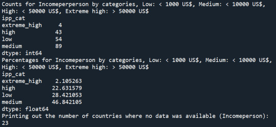
About 46,8 % of the countries fell into the medium category (income per person between 1000 and 10000 US$) while in 54 countries the income per person is less than 1000 US$. 23 countries were not regarded due to missing data.
Variable name: lifeexpectacy Description: 2011 life expectancy at birth (years) As this variable is continuous numerical variable so it can assume an infinite number of real values within a given interval. For proper interpretation categories had to be created. Low: below 60 years Medium: between 60 and 70 years High: between 70 and 80 years Extreme high: over 80 years
Result:

About 48,2 % of the countries fell into the high category (Life expectancy between 70 and 80 years) while in 38 countries the Life expectancy is less than 60years. 22 countries were not regarded due to missing data.
0 notes
Text
Data Management and Visualization (week1 - Life expectancy)
Background: After looking through the codebook for the GapMinder study, I have decided that I am particularly interested in the life expectancy. I included those relevant variables (Democracy score and Income per person) in my personal codebook which I think influences the Life expectancy. I am wondering whether the level of Democracy (non-material) or the Income per person (material) have bigger affect on the Life expectancy in countries.
Literature review: Life expectancy and Non-material assets (Democracy score) and Material assets (Income per person) Search terms used: "life expectancy democracy" and "life expectancy personal income"
There are studies investigating the effect of Democracy levels of the countries along with socioeconomic factors on the population health. These studies confirms correlation between the socioeconomic position and the health outcomes while also arguing that democracy can have an impact on health independently of the effects of socio-economic factors, it is the direct effect of democracy. The findings support the positive influence of democracy on population health (both direct and indirect effect). Although some of them revealed Incoherent polities do not have any significant health advantage over autocratic polities as the reference category.
Hypothesis: My hypothesis is that life expectancy is mostly a function of people's wealth, which ensures their access to a healthy lifestyle (living environment, nutrition, work-life balance) and health care and the level of democracy affects life expectancy only indirectly through wealth.
Reference:
"Is Democracy Good for Health?" Jalil Safaei Volume 36, Issue 4 https://doi.org/10.2190/6V5W-0N36-AQNF-GPD1
"Income distribution and life expectancy." R. G. Wilkinson BMJ. 1992 Jan 18; 304(6820): 165–168.
1 note
·
View note