juniperpublishers-biostatistics - Tumblr blog

juniperpublishers-biostatistics · 6 years ago

Text

Biometrics Technologies for Secured Identification and Personal Verification

Authored by Eludire AA*

Abstract

Biometrics technologies are becoming the foundation of an extensive array of highly secure identification and personal verification solution. It is an automated method of recognizing an individual based on physiological or behavioural characteristics such as fingerprints, distinctiveness in terms of characteristics, persistence characteristics, collectability characteristics and the ability of the method to deliver accurate results under varied environmental circumstances, acceptability, and circumvention. Biometrics technology is useful in the securing of electronic banking, financial and investment transactions, retail sales, social and health services, law enforcement. This paper examines a number of technologies for highly secured identification and personal verification.

Abbreviations: RFID: Radio Frequency Identification Devices; PIN: Personal Identification Number

Introduction

The applications of biometric technology have attracted increasing attention over the past years because of advances in computations and imaging, the identification of criminals reduced identity theft or forgery and enhanced security in electronic transaction and so forth. A number of technologies that are jointly used with automatic data capture to help machines identify objects or individuals for the purpose of increasing efficiency, reducing data entry errors are broadly referred to as Automatic identification or Auto ID. Biometrics is the use of Auto ID capability to recognize a person using different traits that can be captured or presented as data. In technical terms Biometrics is the automated technique of measuring the physical characteristics or personal trait of an individual 2 and comparing that characteristics or trait to a database for the purpose of recognizing that individual. In other words, biometrics can be used for verification as well as for identification. The verification is referred to as «one to one» matching while identification is known as «one-to-many» matching [1].

In using biometric verification two main individual features are employed: unique physiological trait or behavioural characteristics Physiological traits are stable physical characteristics with measurement that is essentially unalterable. Examples of physiological traits include individual’s physical features such as fingerprint, retina, palm prints and iris patterns. Typical examples of behavioural characteristic include individual’s voice, signature, or keystroke dynamics. It can be stated behavioural characteristics are easily influenced by both regulated actions and less regulated psychological factors. Because behavioural characteristics can change over time, the enrolled biometric reference template must be updated each time it is used. From the point of measurement reliability, greater accuracy and security is provided by biometrics based on physiological traits while behaviour-based biometrics can be less costly and less threatening to users. In any case, both techniques provide a significantly higher level of identification than passwords or cards alone. Biometric traits are unique to each individual; they can be used to prevent theft or fraud. Unlike a password or Personal Identification Number (PIN), a biometric trait cannot be forgotten, lost, or stolen. Today there are over 10,000 computer rooms, vaults, research labs, day care centres, blood banks, ATMs and military installations to which access is controlled using devices that scan an individual’s unique physiological or behavioural characteristics. Biometric authentication technologies currently available commercially or under development include fingerprint, face recognition, keystroke dynamics, palm print, retinal scan, iris pattern, signature, and voice pattern [2].

Mode of operation

Biometrics has been used throughout the human history. Kings of Babylon have used handprints to identify different things such as engraving and the like of their own. Depending on the context, a biometric system may operate either in verification mode or identification mode [3]. Evangelista Purkinije from Czech had realized from had realized fingerprint to be unique form of identification in 1823. Fingerprint was first begun to be taken in ink on dactlograms by a by Scotland Yard and the concept of fingerprinting has been unique identifier to catch criminals that took off from the Scotland Yard. In 1970's electronic reader was being developed that led to today's technologies, Sandia National Laboratories has developed hand geometry readers in 1985 and the US government has purchased the readers.

Types of biometrics

The common biometrics based on physiological or behavioural characteristic that a normal person have are:

a. Face

b. Iris

c. Retina

d. Voice

e. Handprint

f. Fingerprint

g. Signature

h. DNA pattern

i. Sweat pores

Basically, the biometric method of identifying a person is preferred over traditional methods. As the use of computer in information technology areas is rapidly increasing, a secure restricted access to privacy or personal data must be obtained. The biometric technique can be used in many application area in order to prevent unauthorized access to use the privacy data such as ATMs, smart card, computer networks, time & attendance system, desktop PCs and workstation. Nowadays, there are several types of system developed with biometrics techniques for real-time identification. The face recognition and fingerprint matching are the most popular biometric techniques used to develop the system followed by hand geometric, iris, retina, and speech. The oldest biometric technique is the electronic fingerprint recognition which has undergone researches and development to extend its applications since its applications by law enforcement. There are two related matching techniques, which are minutiae-based, and correlation- based. What makes a fingerprint unique includes three main patterns; the loop the whorl and the arc using these patterns to match a fingerprint will generally locate a positive identification [4].

The finger print biometric machine is an automated digital version of the old ink and-paper method used for more than a century for identification, primarily by law enforcement agencies. The digital version involves electronically reading users finger print when placed on a platen where the details are mined by the biometric machine algorithm and a finger print pattern analysis is performed. A fingerprint is an impression of the friction ridges on all parts of the finger and pattern recognition algorithms rely on the features found in the impression. These are sometimes known as «epidermal ridges» which caused by the underlying interface between the dermal papillae of the dermis. Gorman identified three major areas where finger print biometrics are used to include: Law enforcement purposes, fraud prevention in entitlement programs, and physical and computer access generally referred to as large-scale Automated Finger Print Imaging Systems (AFIS). It is believed that no two people have identical fingerprint in world, so the fingerprint verification and identification is most popular way to verify the authenticity or identity of a person wherever the security is a problematic question. The reason for popularity of fingerprint technique is the uniqueness of a person arising from his behaviour and personal characteristics which indicates that each and every fingerprint is unique, different from one other.

Finger print recognition is probably the most widely used and well-known biometric that is very less vulnerable to errors in harsh errors environments. Though fingerprint biometrics is applicable in all fields of human endeavour, the finger print of some individuals working in certain industries such as chemical and agricultural are often badly affected making fingerprint mode of authentication problematic. However, to overcome this problem multimodal biometrics system can be applied and fingerprint recognition systems are still considered as the right applications under the right circumstances. Phillips and Martin concluded that finger print biometrics is one of the efficient, secure, cost effective, ease to use technologies for user authentication and according to their survey almost all drawbacks are addressed in fingerprint biometric system.

Verification and identification

Biometric systems operate in two basic modes: verification and identification [5,6]. Verification mode is used to validate a person against whom they claim to be and use one to one matches by comparing biometric data taken from an individual to a biometric template stored in a database. Verification relies on individuals enrolling on the system and registering their identity prior to providing biometric samples which is a massive administrative task when applied to international border control. Identification mode uses a one to many match and searches all the templates in a database to identify an individual therefore the system does not need the compliance of the data subject. The accuracy of biometric technology depends on the accuracy and number of records within the databases.

In the verification mode, the system validates a person’s identity by comparing the captured biometric data with her own biometric template(s) stored system database. In such a system, an individual who desires to be recognized claims an identity, usually via a Personal Identification Number (PIN), a user name, a smart card, etc., and the system conducts a one- to-one comparison to determine whether the claim is true or not (e.g., "Does this biometric data belong to Janet?"). Identity verification is typically used for positive recognition, where the aim is to prevent multiple people from using the same identity.

Identification mode involves establishing a person's identity based only on biometric measurements. The comparator equivalent they obtained biometric with the ones stored in the database bank using a 1: N matching algorithm for recognition. In the identification mode, the system recognizes an individual by searching the templates of all the users in the database for a match. Therefore, the system conducts a one-to-many comparison to establish an individual's identity (or fails if the subject is not enrolled in the system database) without the subject having to claim an identity (e.g., "Whose biometric data is this?"). Identification is a critical component in negative recognition applications where the system establishes whether the person is who she (implicitly or explicitly) denies to be. The purpose of negative recognition is to prevent a single person from using multiple identities. Identification may also be used in positive recognition for convenience (the user is not required to claim an identity). While traditional methods of personal recognition such as passwords, PINs, keys, and tokens may work for positive recognition, negative recognition can only be established through biometrics [3].

Identified application areas

Staff Attendance Management is an area that has been carried out using attendance software that relies on passwords for users’ authentication. However, this type of system allows for impersonation since the passwords can be shared or tampered with. Passwords could also be forgotten at times thereby preventing the user from accessing the system [7]. Oloyede et al. [8] carried out extensive research on applicability of biometric technology to solve the problem of staff attendance. However, the researchers did not write any software to address the problems of attendance [9-12]. Marijana carried out a critical review of the extent to which biometric technology has assisted in controlling illegal entry of travelers into specific country through the integration of biometric passport. The issue regarding how the false acceptance rate can be measured in a border control setting was also looked into. The researcher concludes that the problems associated with biometric technologies such as error rates, spoofing attacks, non-universality and interoperability can be reduced through an overall security process that involves people, technology and procedures. Previously a very few work has been done relating to the academic attendance monitoring problem like radio frequency identification devices (RFID) based systems. Furthermore idea of attendance tracking systems using facial recognition techniques have also been proposed but it requires expensive apparatus still not getting the required accuracy [13-15].

Conclusion

This work presents the biometric technologies that can be used for personal identification and verification. An important area for the application of biometric technologies is implementation of an effective and efficient fingerprint- based Staff Attendance Management System aimed to address the shortcomings in recording staff attendance. This also allow attendance register system generate positive results in the process of gathering, processing and storing attendance information, and making it available for on-line consultation and generation of reports. Having this system enable staff to take their attendance at work serious.

To Know More About Biostatistics and Biometrics Open Access Journal Please Click on: https://juniperpublishers.com/bboaj/index.php

To Know More About Open Access Journals Publishers Please Click on:

Juniper Publishers

#Juniper Publishers #biostatistics #biometrics #open access publishers

0 notes

juniperpublishers-biostatistics · 6 years ago

Text

Prediction of Strong Ground Motion Using Fuzzy Inference Systems Based on Adaptive Networks

Authored by Mostafa Allameh Zadeh*

Abstract

Peak ground acceleration (PGA) estimates have been calculated in order to predict the devastation potential resulting from earthquakes in reconstruction sites. In this research, a training algorithm based on gradient descent were developed and employed by using strong ground motion records. The Artificial Neural Networks (ANN) algorithm indicated that the fitting between the predicted strong ground motion by the networks and the observed PGA values were able to yield high correlation coefficients of 0.78 for PGA. We attempt to provide a suitable prediction of the large acceleration peak from ground gravity acceleration in different areas. Methods are defined by using fuzzy inference systems based on adaptive networks, feed-forward neural networks (FFBP)by four basic parameters as input variables which influence an earthquake in regional studied. The affected indices of an earthquake include the moment magnitude, rupture distance, fault mechanism and site class. The ANFIS network — with an average error of 0.012 — is a more precise network than FFBP neural networks. The FFBP network has a mean square error of 0.017 accordingly. Nonetheless, these two networks can have a suitable estimation of probable acceleration peaks (PGA) in this area.

Keywords: Adaptive-network-based fuzzy inference systems; Feed-forward back propagation error of a neural network; Peak ground acceleration; Rupture distance

Abbreviations: PGA: Peak ground acceleration; ANN: Artificial Neural Networks; FFBP: Feed-Forward Neural Networks; FIS: Fuzzy Inference System; Mw: Moment Magnitude

Introduction

Peak ground acceleration is a very important factor that must be considered in any construction site in order to examine the potential damage that can result from earthquakes. The actual records by seismometers at nearby stations may be considered as a basis. But a reliable method of estimation may be useful for providing more detailed information of the earthquake’s characteristics and motion [1]. The peak ground acceleration parameter is often estimated by the attenuation of relationships and also by using regression analysis. PGA is one of the most important parameters, often analyzed in studies related to damages caused by earthquakes [2]. It is mostly estimated by the attenuation of equations and is developed by a regression analysis of powerful motion data. Powerful motions relating to a ground have basic effects on the structure of that region [3]. Peak ground acceleration is mostly estimated by attenuation relationships [4]. The input variables in the constructed artificial neural network model are the magnitude, the source-to-site distance and the site’s conditions. The output is the PGA. The generalization capability of ANN algorithms was tested with the same training data. Results indicated that there is a high correlation coefficient (R2) for the fitting that is between the predicted PGA values by the networks and those of the observed ones. Furthermore, comparisons between the correlations by the ANN and the regression method showed that the ANN approach performed better than the regression. Developed ANN models can be conservatively utilized to achieve a better understanding of the input parameters and their influence, and thus reach PGA predictions.

Kerh & Chaw [1] used software calculation techniques to remove the lack of certainties in declining relations. They used the mixed gradient training algorithm of Fletcher-Reeves’ back propagation error [5]. They applied three neural network models with different inputs including epicentric distance, focal depth and magnitude of the earthquakes. These records were trained and then the output results were compared with available nonlinear regression analysis. The comparisons demonstrated that the present neural network model did have a better performance than that of the other methods. From a deterministic point of view, determining the strongest level of shaking- that can potentially happen at a site- has long been an important topic in earthquake science. Also, the maximum level of shaking defines the maximum load which ultimately affects urban structures.

From a probabilistic point of view, knowledge of the greatest ground motions that can possibly occur would allow a meaningful truncation of the distribution of ground motion residuals, and thus lead to a reduction in the computed values pertaining to probabilistic seismic hazard analyses. Particularly, it points to the low annual frequencies that exceed norms which are considered for critical facilities [6,7]. Empirical recordings of ground motions that feature large amplitudes of acceleration or velocity play a key role in defining the maximum levels of ground motion, which outline the design of engineering projects, given the potentially destructive nature of motions. They also provide valuable insights into the nature of the tails that further distribute the ground motions.

Feed-forward, back propagation error in neural networks

Artificial neural networks are a set of non-linear optimizer methods which do not need certain mathematical models in order to solve problems. In regression analysis, PGA is calculated as a function of earthquake magnitude, distance from the source of the earthquake to the site under study, local condition of the site and other characteristics that are linked to the earthquake source such as slippery length and reverse, normal or wave propagation. In non-linear regression methods, non-linear relations which exist between input and output parameters are expressed as estimations, through statistical calculations within a specified relationship [8]. One of the most popular neural networks is the back propagation algorithms. It is particularly useful for data modeling and the application of predictions [9] (Equations 1, 2 and 3). It is a supervised learning technique which was first described by Werbos [10] and further developed by Rumelhart et al. [11]. Furthermore, its most useful function is for feed forward neural networks where the information moves in one direction only, forward, beginning from the input nodes through to the hidden nodes, and then to the output nodes. There are no cycles or loops in the network.

In (1), one instance of iteration is written for the back propagation algorithm. Where Xk is a vector of current weights and biases, gk is the current gradient and a is the learning rate.

In (2), where F is the performance function of error (mean square error),'t' is the target and 'a' is the real output

In (3), 'a' is the net output,(n) is the net input and 'f' is the activation function of the neuron model

In (4), the error of energy is calculated by the least squares estimate for back-propagation learning algorithm. Where N is the number of training patterns, m is the number of neurons in the output layer. And tjk is the target value of processing the neuron. Therefore, this algorithm changes synaptic weights along with the negative gradient of the error energy function. Furthermore, it mostly benefits feed-forward neural networks where the information moves in only one direction, forward, beginning from the input nodes, through to the hidden nodes, and then to the output nodes. There are no cycles or loops in the network. The basic back-propagation algorithm adjusts the weights in the steepest direction of descent wherein the performance function decreases most rapidly. This network is a general figure of a multi-layer Prospectron network with one or several occasions of connectivity. Theoretically, it can prove every theorem that can be proven by the feed-forward network. Also, problems can be solved more accurately by testing general feed-forward networks.

Results of FFBP neural network

In Figure 1, testing the output of feed-forward neural networks against the true output is demonstrated. In Figure 2, the correlation coefficient of training, testing and validating general feed-forward neural networks is shown. In Table 1, testing the output of a feed-forward network against its true output has been compared. In Figure 3, training and validating the error graph against the feed-forward neural network is shown. Mean square error versus epoch is shown in Figure 4 with the aim of training and checking the general feed-forward

network. The sensitivity factor was obtained by training the feed-forward network (Figure 5). The sensitivity factor for input parameters is shown in Table 2. The performance error function was obtained by testing the FFBP neural network (Table 3).

Data processing

The datasets of records by large amplitude considered in this study involves one sets of accelerogram selected based on their value of PGA. These records are described below in terms of the variables generally considered to control the behavior of ground motions in general i.e. Magnitude, Rupture distance, style of faulting and site classification. The dataset includes recordings from events with Moment Magnitude ranging from (5.2-7.7) and rupture distance from (0.3-51.7 km). The SC values in the models were used as (1 to 5) for S-Wave velocity (For (1), Vs>1500 m/s and (5) Vs<180m/s). One Model was developed for each ANN method. This model was developed for estimation of maximum PGA values of the three components. The Focal Mechanism values in this model were used as (1 to 5) that (1: Strike Slip, 2:Reverse, 3:Normal, 4:Reverse oblique and 5: Normal oblique). A program includes MATLAB Neural Network toolbox was coded to train and test the models for each ANN method. All recordings from crustal events correspond to rupture distances shorter than 25km. The horizontal dataset shows a predominance of records from strike-slip and reverse earthquakes. Ground motions recorded on early strong-motions instruments often required a correction to be applied to retrieve the peak motions, Filtering generally eliminates the highest frequencies for motions recorded on modern accelerographs, and thus reduces the observed PGA values. The training of networks was performed using 60 sets of data. Testing of networks was done using 14 datasets that were randomely selected among the whole data. As shown in Figure 6 (a,b), the Mw and RD values of test and train data varied in the range of (5.2-7.7) and (0.3-52 km), respectively, the fault mechanism values were given in the Figure 6c. Figure 6d illustrated the site conditions of train and test data. As seen in this figure the site conditions were commonly soft and stiff soil types. Figure 6e showed the maximum PGA of records of the three components. In ANFIS model, training and the testing of records are shown in Figures 7a,b. Final decision surfaces are shown in Figure 7c. Final quiver surfaces are shown in Figure 7d.

Adaptive network based fuzzy inference system

The fuzzy logic appeared parallel to the growth in evolution of neural networks theory. The definition of being fuzzy can be found in human decision-making. These definitions can be searched by methods related to processing information [12].ANFIS is one of hybrid neuro-fuzzy inference expert systems and it works like the Takagi-Sugeno-type fuzzy inference system, which was developed by Jang [13]. ANFIS has a similar structure to a multilayer feed-forward neural network, but the links in an ANFIS can only indicate the flow direction of signals between nodes. No weights are associated with the links [14]. ANFIS

architecture consists of five layers of nodes. Out of the five layers, the first and the fourth layers consist of adaptive nodes while the second, third and fifth layers consist of fixed nodes. The adaptive nodes are associated with respective parameters, while the fixed nodes are devoid of any parameters [15-17]. For simplicity, we assume that the fuzzy inference system under consideration has two inputs x, y and one output called z. Supposing that the rule base contains two fuzzy if-then rules(6 and 7) of the Takagi & Sugenos [18], then the type-1 ANFIS structure can be illustrated as in Figure 6.

Rule 1: If (x is A1) and (y is B1) then (f = plx + qly + r1) (5)

Rule 2: If(x is A2) and (y is B2) then (f2 = p2 x + q2 y + r2) (6)

Where x and y are the inputs, A, Bi are the fuzzy sets and fi is the output within the fuzzy region specified by the fuzzy rule. Then pi , qiand r are the design parameters that are determined during the training process, in which a circle indicates fixed nodes, whereas a square indicates adaptive nodes.

The node functions which are in the same layer are of the same function family as described below:

In Figure 8, layer (1), every node (i) is a square node with a node function like this: O1i=μAi(x)

The outputs of this layer constitute the fuzzy membership grade of the inputs, which are presented as:

Where x and y are the inputs that enter node (i), A is a linguistic label and m (x),mBi (y) can adapt any fuzzy membership function.(a,b and c) are the parameters of the membership function. As the values of these parameters change, the bell shaped function varies accordingly. In layer 2 (Figure 8), every node is a circle node labeled n. The outputs of this layer can be presented as a firing strength of rule. In layer 3, every node is a circle node labeled N. The 'th’ node calculates the ratio of the ‘ith ’ rules' firing strength to the sum of all rules belonging to the firing strength. For convenience, outputs of this layer will be termed as normalized firing strengths. In layer 4, the defuzzification layer is an adaptive node with one node. The output of each node in this layer is simply a first order polynomial.

Where Wi is the output of layer 3, {pi * * ri} is the parameter set. Parameters in this layer will be referred to as consequent parameters. In layer 5,the summation neuron is a fixed node which computes the overall output as the summation of all incoming signals. The single node in this layer is a circle node labeled E that computes the overall output as the summation of all incoming signals.

Functionally, there are almost no constraints on the node functions of an adaptive network except in the case of a piecewise differentiability. Structurally, the only limitation of network configuration is that it should be of the feed-forward type. Due to minimal restrictions, the applications of adaptive networks are immediate and immense in various areas. In this section, we propose a class of adaptive networks which are functionally equivalent to fuzzy inference systems. The targeted architecture is referred to as ANFIS, which stands for Adaptive Network-based Fuzzy Inference System. ANFIS utilizes a strategy of hybrid training algorithm to tune all parameters. It takes a given input/output data set and constructs a fuzzy inference system which has membership function parameters that are tuned, or adjusted, using a back-propagation algorithm in combination with the least-squares type of method (NAZMY .T.M, 2009). Fuzzy inference systems are also known as fuzzy- rule-based systems, fuzzy models, fuzzy associative memories or fuzzy controllers, when used as controllers. Basically, a fuzzy inference system is comprised of five functional blocks.

a. A rule base containing a number of fuzzy if-then rules.

b. A database which defines the membership functions of the fuzzy sets used in the fuzzy rules.

c. A decision-making unit which performs inference operations on the rules.

d. A fuzzification interface which transforms the crisp inputs into degrees of match with linguistic values.

e. A defuzzification interface which transform the fuzzy results of the inference into a crisp output.

Usually the rule base and database are jointly referred to as the knowledge base. The steps of fuzzy reasoning performed by fuzzy inference systems are:

a. To compare the input variables with the membership functions on the premise part so as to obtain the membership values. (That is the fuzzification step).

b. To combine multiplications or minimizations of the membership values on the premise part so as to yield the firing strength of each rule.

c. To generate the qualified consequence— either fuzzy or crisp — of each rule depending on the firing strength.

d. To aggregate the qualified consequences so as to produce a crisp output. (That is the defuzzification step).

Results ofANFIS network for maximum PGA simulation

In this research, an adaptive neuro-fuzzy inference method was applied to simulate non-linear mapping among acceleration peak conditions. The neuro-fuzzy model included an approximate fuzzy reasoning through a sugeno fuzzy inference system (FIS). The input space was fuzzified by a grid-partitioning technique. A hybrid learning algorithm was selected in order to adapt the model's parameters. Furthermore, a linear-nonlinear regression analyses and neural network model were employed to observe the relative performances. Based on our findings, it can be concluded that the neuro-fuzzy control system exhibits a superior performance, compared to the other employed methods [19,20]. In the developed ANFIS model, input-space fuzzification was carried out via the grid-partitioning technique. Fuzzy variables were divided into four triangular membership functions *i>*2> x3* 3. The 625 fuzzy ‘if-then’ rules were set up where in the fuzzy variables were connected by the T-Norm (AND) apparatus. First order sugeno FIS was selected for the approximate reasoning process. The adjustment of independent parameters was made according to the batch mode based on the hybrid learning algorithm. The ANFIS model was trained for 50epochs until the observed error ceased to fluctuate. The resultant neuro-fuzzy Simulink model structure is illustrated in Figure 9.

The input space contains four parameters- moment magnitude (Mw), rupture distance, fault mechanism and site class. The output contains vertical components of PGA, including 40 records from different regions of the world, 24 records for training, 6 records for checking and 10 records for testing the selected ANFIS network. Sixty training data and sixty checking data pairs were obtained at first. The one used here contains 625 rules, with four membership functions being assigned to each input variable, having total number of 3185 fitting parameters which are composed of 60 premise parameters and 3125 consequent parameters. This section presents the simulation results of the proposed type-3 ANFIS with both batch (off-line) and pattern (on-line) learning. In the first example, ANFIS is used to model highly nonlinear functions, where by results are compared with the neural network approach and also with relevant earlier work. In the second example, the FIS name is PGA1 and the FIS type is sugeno. We used the 'and-or' method for input partitioning. Furthermore, we used ‘wtsum’ and 'wtaver' functions for defuzzification. The ranges of input and output variables- in other words, the target variables- are Mw=(5-8), R=(1.50-80 km), fault mechanism type =(1-5),site class=(1-5) and target range (PGA)=(0.5-2.50). The number of MFs={5 5 5 5}, the MF type=Trimf and G-bell MFs (Figure 9 $10). The result of this simulation is LSE: 0.002 and the final epoch error equals to 0.0000002.

Results of the ANFIS network

The input MFs for initial fuzzy inference system and the MFs of trained FIS are shown in Figure 11 & 12. The rule base for the designed ANFIS is shown in Figure 13. Finally, a trained FIS structure is created from the initial FIS by using the ANFIS GUI editor, which is depicted in Figure 14. Also, by testing the results, one can interpret Table 4. Fuzzy parameters used for training ANFIS are shown in Table 5. Also two membership functions for ANFIS training are shown in Figure 10.

Discussion on Results

Empirical recordings have had a significant influence on the estimation of the maximum physical ground motions that can be possible. Peak ground acceleration is an important factor which needs to be investigated before testing devastation potentials that can result from earthquakes in rebuilding sites. One of the problems that deserve attention by seismologists is the occurrence of earthquakes where of the ground motion acceleration peak unexpectedly appears to be more than 1g (Figure 15-18). Valuable data on some earthquakes have been used by Strasser [6] to investigate the earthquakes' physical processes and their consequences.

Figure 15a &b shows the acceleration and velocity traces of the horizontal components falling into this category for which the recordings were available. Spectra of pseudo-acceleration response, pertaining to damping by 5%, are also shown. All the examined traces are characterized by a very pronounced peak in the short-period (T<0.3s) range of the spectrum. The peak velocities that are associated with these recordings are less than 50cm/s. Slip distribution of focal mechanism for tohoko earthquake in Japan are shown in Figure 15c. The results of Gullo and Ercelebi's [2] research (2007) indicated that the fitting between the predicted PGA values by the networks and the observed ones yielded high correlation coefficients (R2). Furthermore, comparisons between the correlations by the ANN and the regression method showed that the ANN approach performed better than the regression method (Table 6). The developed ANN models can be used conservatively so as to establish a good understanding of the influence of input parameters for the PGA predictions.

In Strasser and Bommer's [6] research, a dataset of recordings was examined. It was characterized by the recordings' large amplitudes of PGA (1g) (Figure 15). A number of physical processes have been proposed in the literature to explain these large ground motions, which are commonly divided into source, path and site related effects. While it is often a matter of convention whether these are considered to be predominantly linked to ground motion generation (source effects) or propagation (path and site effects), particularly in the nearsource region, it is important to distinguish between factors that are event-specific, station-specific and record-specific, in terms of implications for ground motion predictions and thus seismic hazard assessment. This is because only site-specific effects can be predicted for certain, in advance. In the present paper, the ANN algorithm indicated that the fitting between the predicted PGA values by the networks and the observed PGA values could yield high correlation coefficients of 0.851for PGA ( 3). Moreover, comparisons between the correlations obtained by the ANN and the regression method demonstrated that the ANN algorithm performed better than the regressions. The Levenberg-Marquart gradient method which we applied on the training algorithm contributed dominantly to fitting the results well.

It had the potential to carry out training very quickly. Moreover, the network models developed in this paper offer new insights into attenuation studies for the purpose of estimating the PGA. In this study, ANFIS and FFBP models were developed to forecast the PGA in different regions of the world. The results of two models and the observed values were compared and evaluated based on their training and validation performance (Figures 2 & 4). The results demonstrated that ANFIS and FFBP models can be applied successfully to establish accurate and reliable PGA forecasting, when comparing the results of the two networks. It was observed that the value of R belonging to the FFBP models is high (0.78) (Figure 3). Moreover, the LSE values of the ANFIS model — which is 0.012 — were lower than that of the FFBP model (Table 4). Therefore, the ANFIS model could be more accurate than the FFBP model. However, a significant advantage is evident when predicting the PGAvia ANFIS, compared to the FFBP model (Figures 16 & 17). The simulations show that the ANFIS network is good for predicting maximum peak ground acceleration in some regions of the world. Finally, the minimum testing error- obtained for the ANFIS network- is 0.002 and the ultimate epoch error is 0.012 (Table 4). This conclusion shows that the ANFIS network can be suitable and useful for predicting values of peak ground acceleration for future earthquakes. PGA-predicted values versus record numbers for three neural networks are shown in Figure 18 & 19.

Conclusion

In this study, FFBP neural networks and ANFIS were trained so as to estimate peak ground acceleration in an area. The input variables in the ANN model were the magnitude, the rupture distance, the focal mechanism and site classification. The output was the PGA only. In the end, the minimum testing error was obtained for the ANFIS network, which equaled 0.002, and the mean square error for the FFBP neural network equaled 0.017. This conclusion shows that the ANFIS network can be suitable and useful in predicting peak ground acceleration for future earthquakes.

Acknowledgement

I am very grateful to the editors and anonymous reviewers, for their suggestions aimed at improving the quality of this manuscript. I also appreciate professors Strasser and Bommer for granting necessary data to this work.

To Know More About Biostatistics and Biometrics Open Access Journal Please Click on: https://juniperpublishers.com/bboaj/index.php

To Know More About Open Access Journals Publishers Please Click on: Juniper Publishers

#Adaptive-network #fuzzy inference systems #neural network #Rupture distance #Moment Magnitude

0 notes

juniperpublishers-biostatistics · 6 years ago

Text

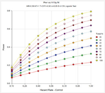
Power Analysis and Sample Size Determination in Log-Rank (Lakatos) Test

Abstract

In this study, it was aimed to investigate the method of calculating the sample size for the Log-rank test developed and proposed by Lakatos (1988) in different scenarios. To that end, Type I error was accepted as 0.05 and the constant hazard rate (p) was accepted as 0.50. The test’s power in different sample sizes was calculated using the Kaplan-Meier method. Through the Monte Carlo simulation method, each situation was repeated 10,000 times, and the results were examined. According to the simulation results the test’s power increased while the total time, sample size and incidence rate increased. When the total incidence rate was 65%, the test’s power reaches up to 80%. In this case, the sample size was above 100. When using the log-rank (Lakatos) test for survival analysis studies, the results of the asymptotic power analyzes were summarized by taking into consideration the situation, group number, total and related event frequency, hazard ratio and test power of different sample scenarios. Sincethe Lakatos method avoids extreme assumption, it provided better results in the simulation study than the other methods requiring assumption.

Keywords:Simulation; Power analysis; Lakatos method; Log-rank test; Sample size

Introduction

The period of time between a given starting time and failure of a living organism or an object is called "lifetime". It is not always possible to find out the lifetime of each patient in clinical trials. Some patients may survive although the trial came to an end, while some may quit the trial or may be excluded from follow-up for some reason. Observations whose survival times are not known due to the specified potential reasons are defined as censored observations [2]. Censored data are encountered in many areas, including medicine, biology, food, engineering and quality control. The most commonly used method for estimating the survival function of a dataset containing censored observations is the Kaplan-Meier method. Kaplan-Meier (KM) method is a non-parametric method that helps calculate the life and death functions without dividing the data on lifetimes into time intervals [3]. Kaplan-Meier method assumes that censored observations and lifetimes are independent of each other. In some cases, more than one survival function can be calculated for patients treated through different methods, and the researcher may wish to test the difference between the survival functions. One of the tests employed to compare survival functions in such cases is the Log-rank test. This test is the most commonly used method for comparing the survival curves in cases where the assumption of proportional hazard is violated [4,5].

In setting up hypotheses in a clinical trial, researchers first determine the population of the research, and then select a random sample, which they think represents the population well, and finally attempt to estimate the population. So, selecting a sample large enough to represent the population is critically important in terms of the reliability and estimation power of the study. It is desired that a planned clinical trial is of an appropriate degree of significance and has a sufficient estimation power. The estimation power is often expected to be higher than 80%. If the power of the test used is low, the test may fall short in detecting a difference that actually exists [6,7]. However, calculation of the actual power of the trial is difficult as it depends on many unknown factors such as censor rate, distribution of lost data, and survival distributions of treatment groups as well as other factors such as stop time, follow-up time, Type I and Type II error rate, and size of impact. This study aims to explore, in different scenarios, the results of the Lakatos method, which is one of the methods where power analysis and sample size calculations in comparing the survival functions of two independent groups.

Methodology

In the study, Type I error was accepted as 0.05 and the constant hazard rate was accepted as 0.50. The test's power in different sample sizes was calculated using the Lakatos method. The scenario is as follows. For instance, the sample size and time interval were accepted to be equal for the treatment groups. Parameters (e.g. 0, , p, ) were calculated for each time interval. Results obtained from repetition of each situation for 10,000 times in the Monte Carlo simulation method were examined. The sample sizes were calculated using PASS (Version 11) program [8].

Lakatos method

The method developed and suggested by Lakatos [9] is based on the assumption that the occurrence of an expected event has an equal weight in all times and that the hazard rates for individuals in different groups are the same in all times [10]. Recording time, follow-up time, and time-dependent hazard rates are used as parameters. This method is based on the Markov model with the variance of the log-rank statistic and an asymptotic mean. In this method, power can be calculated for four different cases, namely, hazard rates, median survival time, survival rate and mortality rate. In this study, the power is calculated for the hazard rates.

The parameter hazard rate is determined individually for the control group and the treatment group. The median survival time (MST) is determined and can be converted into hazard rates using the following relationship:

The parameter survival rate indicates the rate of survival up to T0 (constant time point) and can be converted into hazard rates using the following relationship: .

The parameter mortality rate indicates the rate of mortality up to T0 and can be convertedinto hazard rates using the following relationship:

The proportional hazard assumption may be violated in calculating the power and sample size for the Log-rank statistic. In this case, the sample size formula based on the Markov Process, suggested by Lakatos, can be used. In this process, the survival model contains the following parameters: noncompliance, loss of follow-up time, drop-in, and delay of treatment's effectiveness over the course of the trial. The expected value and variance of the Log-rank statistic is calculated using the hazard rates and the risk rates in each different interval. Lakatos stated that in order to calculate the sample size, the trial period needs to be divided into N equal intervals. The interval should be long enough to fix the number of patients under risk and risk rate in each interval. The sample size required to obtain the test's power (1-p) can be calculated by Equation (1) below, where 0k is the hazard rate of the incident in the kth interval, k is the ratio of patients under risk in the two treatment groups in the kth interval, dk is the number of deaths that occurred in the kthinterval, and d is defined as

Results and Discussion

The simulation results obtained are given in Table 1 & 2. The test’s power increased while the duration of the trial (recording time), sample size and incidence rate increased. The same results can be seen in Figure 1 & 2 as well. When the cumulative incidence is approximately 65% and the sample size is 100 in the recording time 1, the test's power reaches up to 80%. When the cumulative incidence is approximately 73% and the sample size is 100 in the recording time 2, the test’s power is approximately 84%. Therefore, the power value increases while the survival rate in the control and treatment groups increases.

Conclusion

Calculation of sample size is a very critical stage in clinical trials. However, this stage is often bypassed due to complexity of the procedures, which may affect the reliability of the results and result in wasted time and resources used in implementing the clinical trial. In survival analyses, log-rank test is often used to compare two treatment groups. In the present study, a simulation was carried out, and the test's power was assessed through the Lakatos method, one ofthe log-rank tests, in different sample sizes. In calculating the power of the test, the hazard rate was accepted to be 0.50 and the type I error was accepted to be 0.05. Power values were calculated for the different values of recording time, cumulative incidence, and survival rates of groups. According to the results, when the recording time is 1, the test's power is approximately 80%, whereas the recording time increases, the power value rises above 80%. Thus, the test’s power increases while the recording time increases. Also, as the cumulative incidence, sample size and survival rate increase, the test's power increases as well. As can be seen in Figure 2, when thetest’s power is above 80%, the sample size is above 100.

In a simulation study conducted by Alkan et al. [6], it was shown that as the recording time increased, the sample size increased as well in order to achieve a power above 80%. Sample sizes for achieving a power above 80% were found to be 270, 310 and 410. In their simulation study, Lakatos & Lan [1] calculated the test's power to be approximately 90% as the sample size and incidence rate increased. Therefore, they noted in their studies that the Lakatos method gives more accurate results compared to other methods, particularly under the assumption of nonproportional hazard. In conclusion, working on a sample size smaller than what is required in scientific studies decreases the power of the study results, whereas working on a sample size larger than what is required means a waste of time and resources. Thus, by determining an optimum sample size in accordance with the research hypothesis in the beginning of the study, it is possible to ensure the reliability of the study results and prevent the waste of resources.

To Know More About Biostatistics and Biometrics Open Access Journal Please Click on: https://juniperpublishers.com/bboaj/index.php

To Know More About Open Access Journals Publishers Please Click on: Juniper Publishers

#Juniper Publishers #biostatistics #biometrics #Lakatos method #Power analysis

0 notes

juniperpublishers-biostatistics · 6 years ago

Text

On A Boundary Value Problem for A Singularly Perturbed Differential Equation of Non-Classical Type

Abstract

In a semi-infinite strip we consider a boundary value problem for a non-classical type equation of third order degenerating into a hyperbolic equation. The asymptotic expansion of the problem under consideration is construction is constructed in a small parameter to within any positive degree of a small parameter.

Introduction

Boundary value problems for non-classical singularly perturbed differential equations were not studied enough. We can show the papers devoted to construction of asymptotic solutions to some boundary value problems for non-classical type differential equations [1-3].

In this note in the infinite semi-strip we consider the following boundary value problem

Where &>0 is a small parameter, is the given function.

The goal of the work is to construct the complete asymptotics in a small parameter of the solution of problem (1)-(3). When constructing the asymptotics we follow the M.I. Vishik LA & Lusternik [4] technique.

The following theorem is proved.

Theorem

where the functions Wi are determined by the first iterative process, Vj are the boundary layer type functions near the boundary x=1 determined by the second iterative process, en+1 Z is a remainder term, and for z we have the estimation

Where c1>0, c2>0 are the constants independent of e. References.

To Know More About Biostatistics and Biometrics Open Access Journal Please Click on: https://juniperpublishers.com/bboaj/index.php

To Know More About Open Access Journals Publishers Please Click on: Juniper Publishers

#Singularly Perturbed #Non-Classical Type #semi-infinite strip #boundary value #non-classical singularly

0 notes

juniperpublishers-biostatistics · 6 years ago

Text

The Deteriorating State of Methods Development

Authored by William CL Stewart*

Methods development is an important aspect of almost every major quantitative discipline (e.g. Statistics, Biostatistics, Mathematics, Machine Learning, etc.). It is primarily concerned with the creation, implementation, distribution, and maintenance of theoretical and empirical findings. Many of the most useful methods are implemented in the form of computer programs that solve complex quantitative problems for the larger research community. By establishing new methods-an enterprise that requires both art and science, a critical bridge between theory (i.e. theorems, corollaries, and lemmas) and application (i.e. data analysis) is formed. Unfortunately, methods development in modern times has been in a constant state of decline. For the last two decades, it has been -- and continues to be- attacked from four different directions: funding, development time, exposure (in the context of peer-reviewed publications), and most importantly, maintaining training and deployment of the people who can do the work. Let's examine each factor in detail.

Funding

In the 1990's, the NIH (National Institutes of Health) routinely funded grants to develop new methods through many of its centers and institutes (e.g., NIMH, NIDDK, NCRR, and NHGRI). However, by 2011 funding for methods development had been so severely cut that NCRR (National Center for Research Resources) was abolished entirely [1]. Interestingly, NCRR was replaced by NCATS (the National Center for Advancing Translational Science), which is chiefly concerned with funding clinical trials and other kinds of clinical research, not methods grants.

Development time

Methods development is almost always put at the service of some popular technology. In the fields of Statistical and Population Genetics for example, that means "genome sequencing". However, the rapid evolution of DNA-related technologies makes most newly emerging methods "out-ofdate" shortly after they appear in print. Moreover, the combined effect of rapidly evolving technologies and reduced funding can be devastating in terms of shrinking the available time for developing new methods. As such, the window for success is incredibly short, which means that methods don’t get developed and problems don’t get solved.

Exposure

Sadly, almost every high-impact journal in the quantitative sciences has pushed Methods sections to the back of the research article (or possibly even to an Appendix or Supplementary Material), while allowing only a very limited amount of space for exposition, as though the methods used are the least important part of the work and trivial to understand. On the contrary, Methods sections should be at the forefront of the presentation of any scientific work, especially when the methods play a vital role in shaping the final results.

Who does the work

With the dual insults of stark reductions in the training of the next scientific generation, and "encouraged" retirements for senior investigators who are "not productive enough" (i.e., insufficient grant funding), the so-called "next-generation" of methods developers is both poorly mentored and poorly funded, and is perhaps weaker now than ever before [2,3]. In fact, there is a troubling counter culture among young methods developers that is far more concerned with whether a new method works, than with understanding why and how it works. This paradigm shift, albeit subtle, is of the utmost import. If we continue down this path, where methods are selected from a drop-down menu but never developed, then we will find ourselves in a position where there is no one to learn from, we will be unable to incorporate new knowledge with our accepted understanding, and ultimately science will cease to advance [4].

This is why we need to encourage and support methods development, especially by developers who are trained to understand the problems on which they work. A robust methods development infrastructure empowers science by creating an array of tools and ideas to solve real problems. In particular, well-trained developers can often find synergistic approaches that liberate research efforts from simple prediction and imputation. This in turn moves researchers away from findings that are statistically significant but clinically and/or scientifically uninteresting. In summary, if we want to start thinking "outside of the box" again, and if we want to look somewhere other than "beneath the streetlight", then we must commit now, and wholeheartedly to a massive revitalization effort that restores methods development before it's too late [5].

Acknowledgement

I would like to thank Dr. David A Greenberg, and Dr. Veronica J Vieland for their thoughtful comments and valuable insights, both of which substantially improved the clarity and accessibility of this manuscript.

To Know More About Biostatistics and Biometrics Open Access Journal Please Click on: https://juniperpublishers.com/bboaj/index.php

To Know More About Open Access Journals Publishers Please Click on: Juniper Publishers

#Juniper Publishers #biostatistics #biometrics #open access journals

0 notes

juniperpublishers-biostatistics · 6 years ago

Text

Cross-Sectional Data with a Common Shock and Generalized Method of Moments

Authored by Serguey Khovansky*

Abstract

This note outlines possible issues that arise when a common shock exists in such data which models are estimated using Generalized Method of Moments. It provides a theoretical foundation of the issue, an approach to its solution and a reference to an empirical application.

Keywords: Generalized method of moments; Common data shock; Single cross-section of data

Introduction

Cross-sectional data generated at the same point in time may be affected by an exogenous stochastic common shock that influences all data units, perhaps, to a varying extent. Such data generating processes can be found in environmental, ecological and agricultural sciences as well as in economics and finance. For example, storms, floods, droughts, and earthquakes impact the development of biological systems consisting of many individual species. Shocks in the energy markets bring about changes in the production costs of firms across many industries. Interest rate shocks may be responsible for the consumption and savings decisions of many households. Technological shocks affect the evolution of ecosphere. Legal and political shocks may change the perspectives of business firms.

From the econometric point of view, a key consequence of a stochastic common shock shared by all population units is the loss of independence among individual observations, even at the asymptotic level. As a result, the standard versions of the laws of large numbers and central limit theorems become inapplicable. Consequently, the common shock makes inappropriate the regular estimation methods, e.g. GMM (Generalized Method of Moments). This happens, for example, because the large-sample properties of the estimators become dependent on the common shock and lose consistency. To be more precise, the classical GMM consistency proof of Newey & McFadden [5], is valid only for such data where dependence declines as the "distance" between them increases, i.e. even when a shock is present it should not be shared by all population units for the proof to be applicable. Thus, it is very plausible that statistical models based on GMM that do not take the common shock into account (when it indeed exists) end up with inconsistent estimates.

How to address the presence of a common shock shared by all population units? It is only intuitive that the shock must be included in the estimating procedure as a conditioned variable. As is well known, under certain circumstances unconditionally dependent events might be conditionally independent. To be more specific: If two events A and B are dependent, then Pr (A ∩ B) ≠ Pr (B) Pr (A).However, it is possible that there exists an event S with Pr(S > 0) such that conditioning on it the events A and B become independent, i.e. Pr (A ∩ B) = Pr (B) Pr (A).

Generally, theoretical and empirical research about the effect of stochastic common shocks on properties of cross-sectional estimators has received limited attention in the literature, especially in the case of GMM estimators. To a certain extent, this negligence can be explained by computational difficulties associated with estimation procedures that account for the presence of such a shock. Conley [1] examines cross-sectional GMM estimation under a version of a common shock, that is not shared by all population units. Andrews [2] looks at properties of ordinary least squares (OLS) estimators in a setting where common shocks may be present. Andrews [3] also studies properties of instrumental variable (IV) estimators and proposes a set of regularity conditions under which GMM estimators are consistent. Khovansky & Zhylyevskyy [4] suggest a modified GMM estimator and provide conditions under which these estimators are consistent. To implement the proposed GMM estimation approach, a realization of the stochastic common shock must be observed. The essential feature of the method is that it uses conditional rather than unconditional statistical moments. The conditioning is implemented on the sigma-field σX0) generated by a common shock X0 i.e. the GMM objective function is

with the estimate given by The variable Xo and the variables x1, x2,,... are all stochastic. Also, the realization of the random variableX1, X2,...,...Xn. is revealed simultaneously with the realizations of the other random variables. It should be emphasized that in this case the textbook consistency proof of Newey & McFadden [5] is not valid because the GMM objective function Q(θ) converges to a stochastic, rather than deterministic, function. By employing this approach, we can estimate some parameters of a time-series model using currently available cross-sectional data instead of historical time-series. The estimates obtained in this way would reflect the most recent data rather than the past history. Such a course may be appropriate when historical data are irrelevant for the description of the current empirical situation.

Khovansky & Zhylyevskyy [6] give a concrete empirical application which illustrates the use of the proposed estimator. It explores a financial market model comprising a cross-section of stocks and a market portfolio index. In the model, the common shock is represented by the price dynamics of the market index (which reflects the systematic risk) that induces cross-sectional dependence among individual stock returns. In addition to that, the individual stock returns are affected by stock-specific stochastic, i.e. idiosyncratic, risks. An additional important detail is in order. The effect of a common shock on each specific unit may depend on that unit, i.e. vary across the units. To model this heterogeneity appropriately, we might design this dependence as a random variable with some distribution and then, as in the case of GMM, integrate it out by applying the law of iterated expectation.

Future work

Aside from such conventional questions as asymptotic distribution, the Wald test and overidentifying restrictions test in the presence of a common shock, there is also an interest in the question of when and specifically how we should take a common shock into account when dealing with regressions (e.g. in order to obtain consistent estimates). The issues of weak identification, small sample properties, the simulated method of moments and indirect inference are other possible research extensions.

#method of moments #Common data shock #Single cross-section of data #Cross-sectional data #biostatistics #biometrics

0 notes

juniperpublishers-biostatistics · 6 years ago

Text

A Review on the Assessment of the Spatial Dependence

Authored by Pilar Garcia Soidan*

Abstract

For intrinsic random processes, an appropriate estimation of the variogram is required to derive accurate predictions, when proceeding through the kriging methodology. The resulting function must satisfy the conditionally negative definiteness condition, both to guarantee a solution for the kriging equation system and to derive a non-negative prediction error. Assessment of the resulting function is typically addressed through graphical tools, which are not necessarily conclusive, thus making it advisable to perform tests to check the adequateness of the fitted variogram.

Keywords : Intrinsic stationarity; Isotropy; Variogram

Introduction

When spatial data are collected, construction of a prediction map for the variable of interest, over the whole observation region, is typically addressed through the kriging techniques [1]. This methodology has been applied in a variety of areas (hydrology, forestry, air quality, etc.) and its practical implementation demands a previous estimation of the data correlation. The latter issue can be accomplished by approximating the variogram function [2], under the assumption that the underlying process is intrinsic, which is the least restrictive stationarity requirement.

However, estimation of the variogram is far from simple. It requires that the resulting function is valid for prediction, namely, that it fulfills the conditionally negative definiteness condition and, in practice, this problem is usually solved through a three-step procedure [3]. To start, a nonparametric method can be employed to obtain the empirical variogram or a kernel- type approach, among other options, although the functions derived in this way are not necessarily valid [4,5]. Then, in a second step, a valid parametric model is selected, so that the unknown parameters are estimated to best fit the data by any of the distinct criteria (maximum likelihood, least squares, etc.) provided in the statistics literature. Finally, the adequateness of the fitted variogram function should be checked, by using a cross-validation mechanism or goodness of fit tests. The former procedures are not always conclusive and their use is recommended for comparison of several valid models, rather than for assessment of a unique fit. Also, we could perform a test to determine the appropriateness of a variogram model, as the one introduced in Maglione & Diblasi [6], for application to random Gaussian and isotropic random processes, or a more general one suggested in Garcia-Soidan & Cotos-Yanez [7], which accounts for both the isotropic and the anisotropic scenarios.

An important shortcoming of this three-stage scheme is the choice of the parametric model. The most common options are based on the use of flexible functions, such as the Matern one, or on the selection of a model "by eye", by comparing the form of the nonparametric variogram with that derived for different valid families, typically used in practice. However this problem becomes more difficult when dealing with anisotropic variograms. Indeed, isotropy conveys that the data correlation depends only on the distance between the spatial sites and not on the direction of the lag vector, unlike the anisotropic assumption. This means that the assessment of isotropy could be a previous step, whose acceptance would simplify the selection of the model and the subsequent variogram computation. In practice, the isotropic property is typically checked through graphical methods, by plotting a nonparametric estimator in several directions, although the latter procedures are not always determinant. Formal approaches to test for isotropy have been introduced in Guan et al. [8] or in Maity & Sherman [9]. The first test was designed for its application to strictly stationary random processes, whereas the latter one works for more general settings.

Conclusion

The need to obtain an adequate variogram estimator demands a deep exploration of the available data. Firstly the isotropic condition should be checked, as this condition would simplify the characterization of the dependence structure. The graphical diagnosis for assessment of this assumption should be accompanied by the performance of some test to determine its acceptance. Then, a nonparametric estimator can be computed and used to derive a valid parametric fit, whose appropriateness can also be evaluated through any of the goodness of fit tests proposed.

To Know More About Biostatistics and Biometrics Open Access Journal Please Click on: https://juniperpublishers.com/bboaj/index.php

To Know More About Open Access Journals Publishers Please Click on: Juniper Publishers

#Juniper Publishers #open access journals #biostatistics #biometrics #kriging methodology #Variogram #spatial data

0 notes

juniperpublishers-biostatistics · 6 years ago

Text

Analysis of Biological and Biomedical Data with Circular Statistics

Abstract

In this note we will show how circular statistics allow a more accurate and better analysis of several biological and biomedical data sets for which the classical statistical tools may lead to wrong conclusions.

Keywords: Circular data; Directional statistics; von Mises distribution; Structural bioinformatics

Opinion

Several biological and biomedical data sets should by nature be considered as observations lying on the unit circle instead of on a real interval. Studying data on the unit circle requires special care, as the classical statistical concepts no longer hold for such data. Consider for instance the arrival times of patients at a hospital's emergency room or secretion times of certain human hormones. One would naively think of representing histograms of these data on a [0h00; 23h59] interval. To see the first and foremost problem of this approach, consider the problem of analyzing and modeling the secretion times of the hormone melatoninl for patients with sleep disorders. An obvious statistic of interest would be the average time point of melatonin secretion. Say for the sake of simplicity we observed two secretion times, 23h55 and 0h05. Intuitively it is obvious that the time of secretion is concentrated around midnight (0h00), however simply calculating the average time would yield noon (12h00). The reason for this problem lies at the artificial choice of cutting the cycle of a day at midnight (0h00). If we choose for example noon as cut point and represent the data on a [-12h00; 11h59] interval (the times in the interval [12h00; 23h59] are now denoted by the interval [-12h00;-0h01]), our two observations correspond to -0h05 and 0h05 and the average gives the correct value 0h00.

With more data and more spread out data, the art of carefully choosing the cut point will no longer be possible, implying that the traditional mean can no longer be used to calculate an average. This issue can be naturally solved by plotting the data on a unit circle. This allows the natural continuity between any two subsequent times and makes no difference between, say, the passage from 11h15 to 11h16 and the passage from 23h59 to 0h00. The circular mean is then obtained as follows. Suppose we rescale the data to angles θiin[0,2π] radians. These correspond to the points (cos (θi),sin (θi)) on the unit circle. The two-dimensional mean point on the circle corresponds to , where and , leading to the average angle . The latter mean value solves the above-mentioned problems.

Since such a basic concept as the average requires already special care for this type of data, the reader can imagine that all statistical concepts, ranging from descriptive statistics to hypothesis tests, need to be revisited for this type of data. Devising appropriate statistical methods to deal with circular data has grown into an entire research field called circular statistics, and is part of the more general research stream of directional statistics [1]. We have described examples of datasets where the circle was used to represent times. Obviously, it can also be perceived as a compass measuring directions as, e.g., in the study of animal orientation. Probability distributions are the building blocks of statistical methods, and many research efforts, especially in recent years, have been devoted to the study of circular probability distributions. The simplest one is the uniform distribution on the circle with constant density function for all angles θ. It is easy to see that this corresponds to the case where every angle is equally likely.

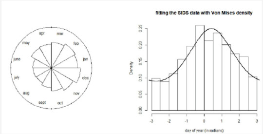
The most notorious probability distribution in circular statistics is undoubtedly the von Mises distribution. It is often viewed as the equivalent of the normal distribution for circular data and its density reads , where μ ∈ [0,2π) is the central location (or mean), the parameter Eq. 1 controls the dispersion of the distribution around π and Io(k) is a normalizing constant. We will briefly illustrate the use of this distribution on data about the Sudden Infant Death Syndrome (SIDS) studied in Mooney et al. [2]. The authors investigated monthly totals of SIDS deaths in England, Wales, Scotland and Northern Ireland for the years 1983-1998, a period including the "Back to Sleep" campaign from the early 1990s that successfully led to a reduction in SIDS deaths. Since there does not exist a natural cut point in the twelve months of a year, these data are by nature circular. We show in Figure 1 the distribution of deaths for the year 1986 both as a rose diagram (a circular histogram) as well as under the form of a more classical histogram, to which we have superimposed the best-fitting von Mises distribution (whose parameters have been estimated by means of maximum likelihood estimation). Mooney et al. [2] have analyzed the evolution of SIDS deaths over the years and investigated whether mixtures of von Mises distributions allow to discover patterns in SIDS mortality rates.

We conclude by providing the reader with an outlook on a hot research topic involving circular statistics, namely the protein structure prediction problem from structural bioinformatics. Predicting the correct three-dimensional structure of a protein given its one-dimensional protein sequence is seen as a holy grail problem. A protein consists of a sequence of amino acids, which essentially defines its three-dimensional shape and dynamic behaviour. Understanding the protein structure at local level represents a key component, and this local structure is adequately described using pairs of dihedral angles per amino acid. In recent years, researchers have made important progresses in this domain by recognizing that these pairs of angles are best described as data on the product space of two circles (a torus) and using the appropriate statistical techniques[3]. Improving further the state-of-the-art statistical tools is very likely to lead to significant further progress in this passionating problem. We hope to have convinced the reader of the usefulness and need to view appropriate biomedical and biological data as observations on the circle. For further reading, we refer the reader to the by now classical book Jammalamadaka & SenGupta[4],as well as to the recent monographs Pewsey et al. [5], focusing on using the software R for dealing with circular data, and Ley & Verdebout [6] which provides an up-to-date account on modern methodologies in the field of directional statistics.

To Know More About Biostatistics and Biometrics Open Access Journal Please Click on: https://juniperpublishers.com/bboaj/index.php

To Know More About Open Access Journals Publishers Please Click on: Juniper Publishers

#Juniper Publishers #biostatistics #biometrics

0 notes