mathsai - Tumblr blog

[mathsai]

Matrices: Examples and Methods

Matrices are fundamental mathematical structures that find applications across various fields, from computer science and physics to economics and engineering. They are a crucial part of linear algebra, a branch of mathematics that deals with vector spaces, linear transformations, and systems of linear equations. In this comprehensive guide, we will explore matrices, their properties, operations, and real-world applications. Whether you're a student seeking to grasp the basics or a professional looking to refresh your knowledge, this guide will provide you with a solid understanding of matrices.

What is a Matrix?

Matrices are rectangular arrays of numbers, symbols, or expressions arranged in rows and columns. They serve as a compact way to represent and manipulate data in various applications, making them a fundamental concept in linear algebra. 

Definition and Notation:

A matrix is usually denoted by a capital letter, such as A, and is described by its dimensions: m × n, where m represents the number of rows, and n represents the number of columns. The individual elements of a matrix are typically denoted using subscripts, e.g., a_ij represents the element in the i-th row and j-th column of matrix A.

Types of Matrices:

Matrices come in various types, including square matrices (m = n), row matrices (1 × n), column matrices (m × 1), and rectangular matrices (m ≠ n). Other specialized types include diagonal matrices, symmetric matrices, and skew-symmetric matrices.

Matrix Size and Elements:

The size of a matrix is determined by the number of rows and columns it possesses. For example, a 2 × 3 matrix has two rows and three columns. Matrix elements can be real numbers, complex numbers, or even functions.

Examples:

Identity Matrix: An n × n square matrix with 1s on the main diagonal and 0s elsewhere.

I = | 1 0 0 |

 | 0 1 0 |

 | 0 0 1 |

Zero Matrix: A matrix where all elements are 0.

O = | 0 0 0 |

| 0 0 0 |

Matrix Operations

Matrices support several fundamental operations that enable us to manipulate and analyze data efficiently.

Addition and Subtraction:

Matrices of the same size can be added or subtracted element-wise. In this operation, corresponding elements are combined.

Example:

A = | 1 2 |

    | 3 4 |

B = | 5 6 |

    | 7 8 |

A + B = | 1+5 2+6 |

        | 3+7 4+8 |

      = | 6 8 |

        | 10 12 |

Scalar Multiplication:

A matrix can be multiplied by a scalar (a single number), which involves multiplying each element by that scalar.

Example:

A = | 1 2 |

    | 3 4 |

2A = | 2*1 2*2 |

     | 2*3 2*4 |

   = | 2 4 |

     | 6 8 |

Matrix Multiplication:

Matrix multiplication is a fundamental operation that combines two matrices to produce a new matrix. It is defined for matrices where the number of columns in the first matrix matches the number of rows in the second matrix.

Example:

A = | 1 2 |

    | 3 4 |

B = | 5 6 |

    | 7 8 |

A * B = | (1*5 + 2*7) (1*6 + 2*8) |

        | (3*5 + 4*7) (3*6 + 4*8) |

      = | 19 22 |

        | 43 50 |

Transposition:

The transpose of a matrix is obtained by swapping its rows and columns. If A is an m × n matrix, then its transpose, denoted as A^T, is an n × m matrix.

Example:

A = | 1 2 3 |

    | 4 5 6 |

A^T = | 1 4 |

      | 2 5 |

      | 3 6 |

Determinants:

The determinant is a scalar value associated with a square matrix. It is used to determine whether a matrix is invertible and plays a crucial role in solving systems of linear equations.

Example:

A = | 2 3 |

    | 1 4 |

det(A) = (2*4) - (3*1) = 8 - 3 = 5

Inverse Matrices:

Square matrices that have non-zero determinants can have inverses. The inverse of a matrix A, denoted as A^(-1), is such that A * A^(-1) = I (the identity matrix).

A = | 2 3 |

    | 1 4 |

A^(-1) = | 4/5 -3/5 |

         | -1/5 2/5 |

Solving Linear Systems 

Matrices are invaluable tools for solving systems of linear equations. This is particularly important in various fields such as physics, engineering, and economics, where systems of linear equations model real-world problems.

Augmented Matrices:

To solve systems linear equations, we often represent them as augmented matrices. Each row in the augmented matrix corresponds to an equation, and the last column holds the constants on the right side of the equations.

2x + 3y = 8

4x + 5y = 14

Augmented Matrix [A|B]:

| 2  3 |  8 |

| 4  5 | 14 |

Row Echelon Form and Reduced Row Echelon Form:

These are special forms of matrices that simplify solving linear systems. In row echelon form, the leading coefficient (the first non-zero element) of each row is 1, and the leading coefficient of each row after the first occurs to the right of the leading coefficient of the previous row. In reduced row echelon form, all entries above and below the leading 1s are 0.

Example (Row Echelon Form):

| 1  2 |  5 |

| 0 -1 | -2 |

Example (Reduced Row Echelon Form):

| 1  0 |  3 |

| 0  1 |  2 |

Gaussian Elimination:

This method transforms an augmented matrix into row echelon form and can be used to solve systems of linear equations.

2x + 3y = 8

4x + 5y = 14

Step 1: Multiply the first equation by -2 and add it to the second equation to eliminate x:

-2(2x + 3y) + (4x + 5y) = -16 + 14

-4x - 6y + 4x + 5y = -2

-y = -2

Step 2: Solve for y:

y = 2

Step 3: Substitute y into the first equation to solve for x:

2x + 3(2) = 8, 2x + 6 = 8 ,2x = 2

x = 1

Matrices Applications

Matrices are not just theoretical constructs; they have a wide range of practical applications across various disciplines.

Graphics and Computer Graphics: In computer graphics, matrices are used to represent transformations like translation, rotation, and scaling. They are pivotal for rendering 2D and 3D graphics.

Data Science and Machine Learning: Matrices play a central role in machine learning, where data is often represented as matrices. Techniques like principal component analysis (PCA) and singular value decomposition (SVD) rely heavily on matrix operations.

Quantum Mechanics: Quantum mechanics leverages matrices, particularly complex Hermitian matrices, to describe quantum states and operators. Matrix representations enable the prediction of quantum behavior.

Matrices are versatile mathematical tools with applications spanning various fields, from science and engineering to data analysis and computer graphics. This comprehensive guide has covered the fundamental concepts of matrices, including their types, operations, and applications. Whether you're solving systems of linear equations, factorizing it, or delving into advanced topics like Hermitian matrices, a solid understanding of matrices is invaluable. We encourage you to explore further and apply this knowledge to your specific area of interest, as it continue to play a vital role in modern mathematics and its practical applications. Unlock the potential of Maths.ai, where AI meets matrices for seamless mathematical exploration and learning

[mathsai]

Sequences and Series: Comprehensive Mathematical Handbook

Sequences and series are fundamental concepts in mathematics that are used in various fields, from calculus and algebra to number theory and statistics. Understanding these concepts is crucial for solving mathematical problems and real-world applications. In this comprehensive guide, we will delve into the world of sequences and series, providing explanations, examples, and methods to help you grasp these concepts thoroughly.

What is a Sequence?

A sequence is an ordered list of numbers or objects, often indexed by natural numbers (1, 2, 3, …). Each element in the sequence is called a term. Sequences can be finite or infinite, and they play a crucial role in various mathematical and scientific disciplines.

Types of Sequences

An arithmetic sequence is a sequence in which the difference between any two consecutive terms is constant. This constant difference is called the common difference (d). The formula for the nth term (an) of an arithmetic sequence is:

an = a1 + (n - 1) * d

Where:

Example 1: Find the 10th term of the arithmetic sequence with a1 = 3 and d = 2.

Using the formula: a10 = 3 + (10 - 1) * 2 = 3 + 9 * 2 = 3 + 18 = 21

A geometric sequence is a sequence in which the ratio between any two consecutive terms is constant. This constant ratio (r) is called the common ratio. The formula for the nth term (an) of a geometric sequence is:

an = a1 * r^(n-1)

Where:

Example 2: Find the 5th term of the geometric sequence with a1 = 2 and r = 3.

Using the formula: a5 = 2 * 3^(5-1) = 2 * 3^4 = 2 * 81 = 162

Special Sequences

The Fibonacci sequence is a famous sequence where each term is the sum of the two preceding ones. It starts with 0 and 1, and the sequence goes like this: 0, 1, 1, 2, 3, 5, 8, 13, 21, …

The formula for the nth Fibonacci number (Fn) can be defined recursively as follows: F1 = 0 F2 = 1 Fn = Fn-1 + Fn-2 for n > 2

A harmonic sequence is a sequence in which each term is the reciprocal of the natural numbers. The general form of a harmonic sequence is:

a_n = 1/n

What is a Series?

A series is the sum of the terms in a sequence. It represents the accumulation of values in a sequence, and there are various types of series, each with its own properties and methods of evaluation.

A. Arithmetic Series

An arithmetic series is the sum of the terms of an arithmetic sequence. The formula to calculate the sum of the first n terms (S_n) of an arithmetic series is:

S_n = n/2 * [2a_1 + (n-1)d]

Where:

Example 3: Find the sum of the first 10 terms of the arithmetic sequence with a_1 = 3 and d = 2.

Using the formula: S_10 = 10/2 * [2 * 3 + (10-1) * 2] = 5 * [6 + 18] = 5 * 24 = 120

B. Geometric Series

A geometric series is the sum of the terms of a geometric sequence. The formula to calculate the sum of the first n terms (S_n) of a geometric series is:

S_n = a_1 * (1 - r^n) / (1 - r)

Where:

Example 4: Find the sum of the first 5 terms of the geometric sequence with a_1 = 2 and r = 3.

Using the formula: S_5 = 2 * (1 - 3^5) / (1 - 3) = 2 * (1 - 243) / (-2) = (2 * (-242)) / (-2) = 242

Convergent and Divergent Series

A series is said to be convergent if the sum of its terms approaches a finite limit as the number of terms increases. Conversely, a series is divergent if the sum of its terms does not approach a finite limit.

Example 5: Consider the series 1 + 1/2 + 1/4 + 1/8 + 1/16 + … This is a geometric series with a common ratio r = 1/2. It is convergent because as n approaches infinity, the sum approaches 2.

Methods of Evaluating Series

A. Finite Sum Formula

Some series have finite formulas that allow you to calculate the sum directly without adding up individual terms. One famous example is the sum of natural numbers:

1 + 2 + 3 + 4 + … + n = n(n + 1)/2

B. Partial Sums

When you cannot find a finite formula for a series, you can use partial sums to approximate the sum. A partial sum is the sum of the first n terms of a series.

Example 6: Approximate the sum of the series 1 + 1/2 + 1/4 + 1/8 + 1/16 + … by calculating the partial sums for n = 1, 2, 3, …

Partial sums: S_1 = 1 S_2 = 1 + 1/2 = 1.5 S_3 = 1 + 1/2 + 1/4 = 1.75 S_4 = 1 + 1/2 + 1/4 + 1/8 = 1.875 …

As you can see, the partial sums get closer and closer to 2, which is the sum of the series.

C. Integral Test

The integral test is a method for determining the convergence or divergence of a series by comparing it to an integral. If f(x) is a positive, continuous, and decreasing function for all x ≥ 1, and if the series is a_n = f(n), then the series and the integral of f(x) from 1 to infinity have the same behavior:

, then the series Σ a_n diverges.

D. Comparison Test

The comparison test is used to determine the convergence or divergence of a series by comparing it to another series with known convergence properties.

E. Alternating Series Test

The alternating series test is used to determine the convergence of a series that alternates between positive and negative terms.

Example 7: The alternating series Σ (-1)^n/n is a classic example of an alternating series. It converges by the alternating series test because the terms are decreasing (1/n+1 ≤ 1/n) and approach zero as n approaches infinity.

F. Ratio Test

The ratio test is a powerful test for determining the convergence or divergence of a series.

Example 8: Consider the series Σ (1/2)^n. Using the ratio test:

lim (as n approaches infinity) |(1/2)^(n+1) / (1/2)^n| = 1/2 < 1

Since the limit is less than 1, the series Σ (1/2)^n converges absolutely.

Sequences and series are essential mathematical concepts with wide-ranging applications in various fields. In this comprehensive guide, we've covered the basics of sequences, including arithmetic and geometric sequences, as well as special sequences like the Fibonacci and harmonic sequences. We've also explored different types of series, including arithmetic and geometric series, and discussed methods for evaluating them, such as finite sum formulas, partial sums, the integral test, comparison test, alternating series test, and ratio test.

Understanding sequences and series is crucial for tackling more advanced topics in mathematics, including calculus and advanced calculus, where these concepts play a central role. Additionally, they have applications in physics, engineering, computer science, and many other disciplines. By mastering the concepts and methods presented in this guide, you'll be well-equipped to handle a wide range of mathematical problems and applications involving sequences and series. Master sequences and series with ease - Maths.ai is your ultimate resource for mathematical excellence.

[mathsai]

Integral Calculus: Examples and Methods

Integral calculus is a fundamental branch of mathematics that deals with the concept of integration. It provides a powerful tool for solving a wide range of problems related to area, volume, accumulation, and various other mathematical concepts. In this guide, we will delve into the basics of integral calculus, explore different techniques of integration, and provide practical examples to illustrate their applications.

The Fundamental Theorem of Calculus:

Integral calculus is closely tied to the concept of differentiation, as expressed by the Fundamental Theorem of Calculus. This theorem establishes a relationship between differentiation and integration, making it a cornerstone of integral calculus.

Definite and Indefinite Integrals:

Integrals can be classified into two main types: definite and indefinite integrals. A definite integral represents the area under a curve between two specific points on the x-axis. An indefinite integral, also known as an antiderivative, represents a family of functions whose derivatives yield the original function.

3. Methods of Integration:

There are various methods to evaluate integrals, each suited for different types of functions. Some common methods include:

a. Substitution Method:

The substitution method involves substituting a variable with a new expression to simplify the integral. This technique is particularly useful for integrals involving composite functions or trigonometric expressions.

b. Integration by Parts:

Integration by parts is derived from the product rule of differentiation. It involves splitting the integrand into two functions and applying a specific formula to evaluate the integral.

c. Partial Fraction Decomposition:

In practice, we utilize this method to break down intricate rational functions into simpler fractions, thus simplifying the integration process. This approach finds frequent application when working with rational functions.

d. Trigonometric Substitution:

Trigonometric substitution is used to simplify integrals involving radical expressions by substituting trigonometric identities to simplify the expression.

e. Improper Integrals:

Improper integrals involve integrating over an infinite interval or a function with an infinite discontinuity. Such integrals are evaluated using limits, and they have applications in various real-world scenarios.

4. Applications of Integral Calculus:

Integral calculus finds extensive applications in various fields, such as physics, engineering, economics, and more. Some notable applications include:

a. Area and Volume Calculations: c

b. Physics and Engineering: Integral calculus is essential for solving problems related to motion, work, energy, and many other physical phenomena.

c. Probability and Statistics: Probability density functions and cumulative distribution functions involve integrals, making integral calculus crucial in the field of statistics.

d. Economics: Integral calculus allows us to determine the area under a curve, calculate the volume of solids formed by revolution, and ascertain the surface area of three-dimensional objects.

5. Practical Examples: Let's explore some practical examples to showcase the methods of integration:

Examples

Substitution Method

Evaluate ∫(2x + 1)^2 dx using the substitution method.

Solution:

Let u = 2x + 1, then du = 2 dx. The integral becomes ∫u^2 (1/2) du, which is a simple power integral.

EIntegration by Parts Evaluate ∫x ln(x) dx using integration by parts.

Solution:

Choose u = ln(x) and dv = x dx. Apply the integration by parts formula: ∫u dv = uv - ∫v du. This leads to the integral ∫x ln(x) dx = (1/2)x^2 ln(x) - ∫(1/2)x dx.

Integral calculus is an indispensable tool for solving a wide range of mathematical problems and has a plethora of applications across various disciplines. From finding areas under curves to solving complex physical phenomena, integral calculus plays a vital role in advancing our understanding of the world. By mastering the fundamental techniques and methods of integration, one can unlock the potential to solve intricate problems and contribute to various fields of study. Explore the power of integral calculus and more with maths.ai - your gateway to mathematical enlightenment.

[mathsai]

Understanding Vector: A Complete Guide

Vector is fundamental mathematical entities used to represent quantities with both magnitude and direction. They find applications in various fields such as physics, engineering, computer graphics, and more. This guide provides a concise overview of vectors, their properties, operations, and applications.

Definition and Notation:

A vector is an ordered collection of numbers, often represented as an arrow pointing from an initial point to a terminal point in space. Each component of a vector corresponds to a direction in a specific dimension.

Components and Representation:

In a three-dimensional space, a vector v can be represented as v = (v₁, v₂, v₃), where v₁, v₂, and v₃ are the components along the x, y, and z axes, respectively. The magnitude (length) of the vector is denoted by ||v|| and is calculated as the square root of the sum of the squares of its components.

Vector Operations:

Addition:

The sum of two vectors u and v is a vector w = u + v, where each component of w is the sum of the corresponding components of u and v.

Subtraction:

The difference between two vectors u and v is a vector w = u - v.

Scalar Multiplication:

The dot product of two vectors, u and v, equals the sum of the products of their corresponding components: u₁v₁ + u₂v₂ + u₃v₃. It yields a scalar value that measures the similarity of the two vectors' directions.

Cross Product (Vector Product):

The cross product of two vectors u and v results in a new vector w = u × v. Its magnitude is ||w|| = ||u|| ||v|| sin(θ), where θ is the angle between u and v=-0=;

Properties of Vector:

Applications:

Engineering:

Vectors help model and analyze forces, moments, and other physical quantities in fields like structural analysis and fluid dynamics.

Computer Graphics:

used to represent points, directions, and transformations, forming the basis for rendering 2D and 3D graphics.

Navigation:

Vectors assist in determining positions, distances, and directions, vital for navigation systems and GPS technology.

Aeronautics:

Vectors help in understanding aircraft motion, wind speed and direction, and navigation.

Machine Learning:

employed to represent features and data points, making them essential for various machine learning algorithms.

Physics:

Vectors are extensively used in physics to describe quantities like force, velocity, acceleration, and electromagnetic fields.

Vectors are essential mathematical tools that describe quantities with both magnitude and direction. They find applications in physics, engineering, computer graphics, navigation, and more. Understanding its properties, operations, and coordinate systems is crucial for mastering their use across diverse fields.

Explore the power of mathematics and AI at Maths.ai. Discover the synergy between algorithms and vector concepts.

[mathsai]

Mathematical Dimensions: An In-Depth Overview

Dimensions are a fundamental concept in mathematics that help us understand the size, shape, and structure of objects and spaces. In this guide, we will explore them in various contexts, from the basic concept of dimension in geometry to higher-dimensional spaces and their applications in real-world scenarios.

Understanding Dimensions:

In mathematics, a dimension is a measure of the number of coordinates required to locate a point within a space. The dimension of a space is closely related to the number of independent directions in which movement is possible.

One-Dimensional Space:

A one-dimensional space is the simplest concept of dimension. Points in one-dimensional space are located using a single coordinate, typically denoted as "x."

Two-Dimensional Space:

A two-dimensional space extends the concept to a plane. It is represented by two coordinates, usually denoted as "x" and "y." Geometry and coordinate geometry extensively deal with two-dimensional spaces.

Three-Dimensional Space:

The fundamental nature of the physical world finds its most accurate description within a three-dimensional spatial framework.In this context, we employ three coordinates, typically referred to as "x," "y," and "z," to establish the precise location of a point.. Here, three coordin. This space allows us to visualize objects with depth, such as cubes, spheres, and other three-dimensional shapes.

Vector Spaces and Linear Algebra:

A three-dimensional space most accurately characterizes the physical realm. The dimension of a vector space is a pivotal metric, denoting the smallest count of vectors essential to collectively span the entirety of the space. This concept finds direct relevance in Euclidean space, where the dimension corresponds to the quantity of coordinates necessary for pinpointing a specific location within that space.

Fractals and Non-Integer Dimensions:

Not all dimensions are integers. Fractals are intricate mathematical structures with non-integer dimensions. Fractal dimension quantifies how space is occupied by fractal entities. The fractal dimension lies between the object's topological dimension (like 1D, 2D, etc.) and its Hausdorff dimension, which quantifies the object's complexity.

String Theory and Extra Dimensions:

In theoretical physics, string theory suggests the existence of more than the usual three dimensions. It proposes that the universe has extra dimensions beyond our perception. These dimensions could be compactified, meaning and they are so small that we don't directly observe them in our macroscopic world.

Practical Applications:

Dimensions have practical applications in various fields, including computer graphics, computer-aided design (CAD), architecture, and more. Understanding dimensions is essential for creating accurate representations of real-world objects and spaces in these domains.

In conclusion, they are a foundational concept in mathematics that underpins our understanding of space, shape, and structure. From one-dimensional lines to multi-dimensional spaces, and dimensions, fundamental tool used across various mathematical disciplines. They have far-reaching applications in the real world, from physics to engineering. As a result of this, we gain a deeper insight into the fundamental nature of our universe. Explore Maths.ai for insightful discussions on diverse mathematical dimensions and their real-world applications.

[mathsai]

Mastering Algebra: An In-Depth Manual

Welcome to the world of algebra, a fundamental branch of mathematics that deals with symbols, letters, and the rules for manipulating these symbols to solve various mathematical problems. Algebra plays a crucial role in both mathematics and everyday life, from solving equations to modeling real-world situations. In this comprehensive guide, we'll cover the essential concepts, provide examples, and explore problem-solving methods in algebra.

Basic Concepts of Algebra

Algebra uses letters (variables) to represent numbers or quantities in equations and expressions. These variables can stand for unknown values, enabling us to solve for them using mathematical operations.

Algebraic Expressions:

An algebraic expression is a combination of numbers, variables, and operations like addition, subtraction, multiplication, and division. For example, `3x + 2y` is an algebraic expression where `x` and `y` are variables.

Equations:

Equations are mathematical statements that assert the equality of two expressions. They involve an equal sign (`=`) and often unknown variables. Solving equations involves finding the values of variables that make the equation true.

Solving Linear Equations:

In linear equations, variables are raised to the power of 1.. The general form of a linear equation is `ax + b = 0`. To solve linear equations, isolate the variable by performing operations that maintain balance on both sides of the equation. For example, to solve `2x + 5 = 11`, subtract 5 from both sides to get `2x = 6`, then divide by 2 to find `x = 3`.

Systems of Equations:

A system of equations consists of multiple equations with the same set of variables. Solving a system involves finding values of variables that satisfy all the equations simultaneously. Methods include substitution, elimination, and matrix methods.

Polynomials:

Polynomials are expressions with one or more terms involving variables raised to non-negative integer powers. They can be added, subtracted, multiplied, and divided using polynomial operations. For example, `3x^2 + 2x - 5` is a polynomial.

Factoring:

Factoring involves breaking down a polynomial into its simpler components (factors). This is useful for simplification and solving equations. For example, factoring `x^2 - 4` yields `(x + 2)(x - 2)`.

Quadratic Equations:

Quadratic equations involve variables raised to the power of 2. The standard form is `ax^2 + bx + c = 0`. They can be solved using methods like factoring, completing the square, and the quadratic formula.

Inequalities:

Inequalities compare two expressions using symbols like `<`, `>`, `≤`, and `≥`. They represent relationships between quantities that are not necessarily equal.

Exponents and Radicals:

Exponents indicate how many times a number (base) is multiplied by itself. Radicals are the inverse operation of exponentiation. They include square roots, cube roots, etc.

Graphing Equations:

Graphs visually represent equations and functions. For linear equations, the graph is a straight line; for quadratic equations, it's a parabola. Graphs provide insights into solutions and relationships.

Applications of Algebra:

Algebra has countless applications in various fields, including physics, engineering, economics, and computer science. It's used to model real-world situations, analyze data, and solve complex problems.

Algebra is a foundational branch of mathematics that plays a vital role in problem-solving and understanding the relationships between quantities. From basic expressions to complex equations, mastering algebraic concepts empowers you to tackle a wide range of mathematical and practical challenges. By following the principles outlined in this guide and practicing with examples, you'll develop the skills to confidently navigate the world of algebra and beyond. Explore the wonders of mathematics with Maths.ai! From algebra to advanced calculus, embark on enlightening learning.

[mathsai]

Know Geometry: Concepts, Examples, and Methods

Geometry is a fundamental branch of mathematics that explores the properties and relationships of shapes, sizes, and space. From basic shapes to complex spatial configurations, geometry plays a crucial role in various fields such as architecture, engineering, art, and science. In this comprehensive guide, we will delve into the core concepts of geometry, provide illustrative examples, and outline essential methods. Whether you're a student seeking to deepen your understanding or an AI-based math enthusiast, this guide will serve as an invaluable resource.

Basic Concepts of Geometric

Geometry begins with fundamental concepts that lay the groundwork for more advanced topics. These include:

Point:

A point is a location in space, represented by a dot. It has no size, shape, or dimensions.

Line:

A line is a straight path that extends infinitely in both directions.

Plane:

A plane is a flat, two-dimensional surface that extends infinitely. At least three non-collinear points determine it.

Angle:

An angle is formed when two rays share a common endpoint (vertex). Angles are measured in degrees or radians.

Types of Angles:

Angles can be classified into various types based on their measurements and relationships:

Acute Angle:

An angle measuring less than 90 degrees.

Right Angle:

An angle measuring exactly 90 degrees.

Obtuse Angle:

An angle measuring more than 90 degrees but less than 180 degrees.

Straight Angle:

An angle measuring exactly 180 degrees.

Reflex Angle:

An angle measuring more than 180 degrees but less than 360 degrees.

Types of Polygons:

Polygons are closed shapes with straight sides. They can be categorized based on the number of sides they possess:

Triangle: A polygon with three sides.

Quadrilateral: A polygon with four sides.

Pentagon: A polygon with five sides.

Hexagon: A polygon with six sides.

Heptagon (Septagon): A polygon with seven sides.

Octagon: A polygon with eight sides.

Nonagon: A polygon with nine sides.

Decagon: A polygon with ten sides.

Congruence and Similarity:

Congruent shapes have the same size and shape, while similar shapes have the same shape but possibly different sizes. Methods to determine congruence and similarity include:

Side-Side-Side (SSS) Criterion:

Two triangles are congruent if their corresponding sides are proportional.

Side-Angle-Side (SAS) Criterion:

If two sides and the included angle of one triangle are congruent to the corresponding sides and angle of another triangle, the triangles are congruent.

Angle-Angle (AA) Criterion:

If two angles of one triangle are congruent to two angles of another triangle, the triangles are similar.

Side-Side-Angle (SSA) Criterion:

SSA is a similarity criterion that requires additional conditions to establish similarity.

The Pythagoras Theorem:

The Pythagoras theorem is a fundamental concept in geometry that relates the sides of a right triangle:

In a right triangle, the square of the length of the hypotenuse (the side opposite the right angle) is equal to the sum of the squares of the lengths of the other two sides.

Example: Consider a right triangle with legs of lengths 3 units and 4 units. The hypotenuse can be calculated using the Pythagorean theorem: (c^2 = a^2 + b^2), where (c) is the hypotenuse, (a) is the first leg, and (b) is the second leg. Substituting the values, we get (c^2 = 3^2 + 4^2), which simplifies to (c^2 = 9 + 16), and finally (c^2 = 25). Taking the square root of both sides, (c = 5). Therefore, the length of the hypotenuse is 5 units.

Coordinate Geometry:

Coordinate geometry involves using algebraic methods to study geometric shapes. It's the bridge between algebra and geometry. The Cartesian coordinate system is used to represent points on a plane.

Distance Formula:

The distance between two points ((x_1, y_1)) and ((x_2, y_2)) in a plane is given by (\sqrt{(x_2 - x_1)^2 + (y_2 - y_1)^2}).

Midpoint Formula:

The midpoint of a line segment between two points ((x_1, y_1)) and ((x_2, y_2)) is (\left(\frac{x_1 + x_2}{2}, \frac{y_1 + y_2}{2}\right)).

Three-Dimensional Geometry:

Geometry extends into three dimensions with concepts such as points, lines, and shapes in space. Common shapes include cubes, spheres, cylinders, and cones.

Trigonometry and Geometry:

Trigonometry is closely related to geometry and involves the study of the relationships between the angles and sides of triangles. Key trigonometric ratios include sine, cosine, and tangent.

Proofs of Geometry

Proofs are essential in geometry to demonstrate the validity of statements and theorems. Different methods of proof include direct proof, proof by contradiction, and proof by induction.

Geometry is a vast field that encompasses diverse concepts, methods, and applications. From understanding basic shapes to exploring complex spatial relationships, geometry plays a pivotal role in various disciplines. This guide has provided an overview of essential concepts, examples, and methods in geometry, empowering learners and AI-based systems to navigate and comprehend this fascinating mathematical realm. By mastering these fundamentals, you'll be well-equipped to tackle more advanced geometric challenges and contribute to the ever-evolving world of mathematics and its applications, use maths.ai to ace your education.

[mathsai]

Statistics: A Complete Guide with Examples and Methods 

Statistics is a branch of mathematics that involves collecting, organizing, analyzing, interpreting, and presenting data. It plays a crucial role in various fields, from science and economics to social sciences and healthcare. In this comprehensive guide, we will explore the fundamental concepts of statistics, provide practical examples, and discuss essential methods commonly used in data analysis.

Descriptive Statistics:

Descriptive statistics involves summarizing and presenting data in a meaningful way.

Measures of Central Tendency in Statistics:

Mean:

The average of a set of values.

Median:

Arrange the data in ascending order and find the middle value.

Mode:

The value that appears most frequently in a dataset.

Measures of Dispersion:

Range:

The difference between the maximum and minimum values.

Variance:

Measures how much the values in a dataset deviate from the mean.

Standard Deviation:

The square root of the variance, providing a measure of the spread of data.

Example:

Consider a dataset of exam scores: 85, 90, 75, 92, 88, 78. The mean is (85+90+75+92+88+78)/6 = 85.33, the median is 86.5, and the mode is not applicable as no value appears more than once.

Probability Distributions:

Probability distributions describe the likelihood of different outcomes in a random experiment. Two common distributions are the normal distribution and the binomial distribution.

Normal Distribution: A bell-shaped curve with a symmetric and continuous nature.

Binomial Distribution: Models the number of successes in a fixed number of independent Bernoulli trials.

Example:

In a normal distribution, around 68% of the data falls within one standard deviation of the mean, and about 95% falls within two standard deviations.

Sampling and Estimation:

Sampling involves selecting a subset of a population for analysis. Estimation techniques allow us to make inferences about the entire population based on the sample.

Random Sampling: Each member of the population has an equal chance of being selected.

Sampling Methods: Stratified sampling, cluster sampling, and systematic sampling.

Example:

To estimate the average height of students in a school, a random sample of 100 students is selected, and their heights are measured. The sample mean is then used to estimate the population mean.

Hypothesis Testing:

Hypothesis testing is used to make decisions about a population based on a sample of data. The process involves setting up null and alternative hypotheses, calculating test statistics, and determining the p-value.

Null Hypothesis (H0): The statement being tested (usually stating no effect or no difference).

Alternative Hypothesis (Ha): The opposite of the null hypothesis.

Example:

A drug company tests a new medication by comparing it to a placebo. The null hypothesis might be that the medication and placebo have no difference in effectiveness..

Correlation Analysis:

Correlation measures the strength and direction of a linear relationship between two variables. The correlation coefficient ranges from -1 to 1.

Example:

A positive correlation between hours of exercise and physical fitness indicates that as exercise increases, physical fitness tends to increase as well.

Chi-Square Test:

The chi-square test assesses the independence between categorical variables. It compares the observed frequencies in a contingency table to the expected frequencies.

Example:

To establish a relationship between gender and music preference, researchers can conduct a chi-square test on survey data.

Statistics is a powerful tool for understanding and interpreting data in various fields. This guide provided an overview of descriptive statistics, probability distributions, sampling, hypothesis testing, regression analysis, correlation analysis, and the chi-square test. By applying these methods, researchers and analysts can draw meaningful conclusions, make predictions, and guide decision-making based on data-driven insights. Visit maths.ai to take help in maths solutions.

[mathsai]

Differentiation: Guide, with Examples and Methods

Differentiation is a fundamental concept in calculus that allows us to understand how a function changes as its input values change. It is a crucial tool in mathematics and has numerous applications in various fields such as physics, engineering, economics, and more. In this comprehensive guide, we will explore the concept of differentiation, delve into its methods, and provide practical examples to help you grasp this important mathematical concept.

Understanding Differentiation:

Differentiation is the process of finding the rate at which a function's output changes with respect to its input. In other words, it measures the slope or steepness of a function at a particular point. The result of differentiation is another function, known as the derivative, which gives the instantaneous rate of change of the original function.

Methods of Differentiation:

There are several methods of differentiation that allow us to find the derivative of a function. Let's explore some of the most common methods:

1. First Principles:

The derivative of a function f(x) at a point x=a can be found using the limit definition:

f'(a) = lim (h -> 0) [f(a + h) - f(a)] / h

2. Power Rule:

For functions of the form f(x) = x^n, where n is a constant, the derivative is given by:

f'(x) = n * x^(n-1)

3. Product Rule:

For the product of two functions u(x) and v(x), the derivative is given by:

(u*v)' = u' * v + u * v'

4. Quotient Rule:

For the quotient of two functions u(x) and v(x), the derivative is given by:

(u/v)' = (u' * v - u * v') / v^2

5. Chain Rule:

For composite functions, where one function is inside another, the chain rule states:

(f(g(x)))' = f'(g(x)) * g'(x)

6. Trigonometric Functions:

Derivatives of trigonometric functions are given by well-defined rules, such as:

 sin'(x) = cos(x), cos'(x) = -sin(x), tan'(x) = sec^2(x), etc.

7. Exponential and Logarithmic Functions:

Derivatives of exponential and logarithmic functions have distinct patterns, such as

 (e^x)' = e^x, (ln(x))' = 1/x, etc.

Some Examples:

Let's illustrate differentiation with some examples:

Example 1 - Power Rule:Find the derivative of the function f(x) = 3x^4.

f'(x) = 4 * 3x^(4-1) = 12x^3

Example 2 - Product Rule:

Find the derivative of the function f(x) = x^2 * sin(x).

f'(x) = (2x * sin(x)) + (x^2 * cos(x))

Example 3 - Chain Rule:

Find the derivative of the function f(x) = e^(2x).

f'(x) = 2 * e^(2x)

Example 4 - Quotient Rule:

 Find the derivative of the function f(x) = (3x^2 + 1) / x.

f'(x) = (2 * 3x * x - (3x^2 + 1)) / x^2

= (6x^2 - 3x^2 - 1) / x^2

= (3x^2 - 1) / x^2

Applications of Differentiation:

Differentiation has wide-ranging applications in various fields:

1. Physics:

In physics, differentiation is used to calculate velocities, accelerations, and rates of change of various physical quantities.

2. Economics:

Differentiation is employed to analyze marginal changes, elasticity, and optimization in economic models.

3. Engineering:

Engineers use this to determine rates of change in voltage, current, and other quantities in electrical circuits.

4. Biology:

Differentiation helps model population growth, analyze biological processes, and understand rates of change in biological systems.

5. Optimization:

Differentiation helps find maximum and minimum points of functions, crucial in optimization problems.

6. Calculus Concepts:

Differentiation is a key step in solving differential equations, which model dynamic systems in mathematics.

Differentiation is a fundamental concept in calculus with broad applications across various disciplines. By understanding its methods and principles, you gain the ability to analyze how functions change, which is essential in understanding real-world phenomena. Through the power of differentiation, you can explore the dynamic and ever-changing nature of the world around us. Visit maths.ai for such contents elated to mathematical concepts.

[mathsai]

Integration: A Comprehensive Guide

Welcome to the comprehensive guide on integration – an essential concept in mathematics that plays a significant role in various fields, including calculus, physics, engineering, and more. In this guide, we will delve into the fundamentals of integration, explore various methods and techniques, and provide practical examples to solidify your understanding.

Introduction to Integration

Integration is a mathematical operation that deals with finding the integral of a function. It is the reverse process of differentiation. It used to calculate quantities like area, volume, work, and many more. The integral of a function represents the accumulation of its instantaneous rates of change.

Basic Concepts of Integration

Before delving into integration methods, it's important to understand the basic concepts:

Antiderivative:

An antiderivative of a function *f(x)* is a function *F(x)* whose derivative is *f(x)*, also known as an indefinite integral.

Integral Symbol:

The integral symbol (∫) is used to represent the integration operation. For instance, ∫(*f(x)*) *dx* represents the integral of *f(x)* with respect to *x*.

Definite and Indefinite Integrals

There are two types of integrals: definite and indefinite.

ndefinite Integral:

The indefinite integral of a function *f(x)* with respect to *x* is denoted as ∫(*f(x)*) *dx* + *C*, where *C* is the constant of integration. It represents a family of functions that differ by a constant.

Definite Integral:

The definite integral of a function *f(x)* from *a* to *b* is denoted as ∫_a^b (*f(x)*) *dx* and represents the net signed area between the curve and the *x*-axis over the interval *[a, b]*.

## 4. Integration Techniques

a. Substitution Method

The substitution method is used when an integral involves a composition of functions. The key idea is to substitute a new variable to simplify the integral.

Example: ∫2x * cos(x^2) * dx

Let *u = x^2*, then *du = 2x dx*. The integral becomes ∫cos(u) * du, which is simpler to solve.

b. Integration by Parts

Integration by parts is a technique based on the product rule for differentiation, used to integrate the product of two functions.

Formula: ∫u * dv = uv - ∫v * du

Example: ∫x * sin(x) * dx

Let *u = x* and *dv = sin(x) dx*. Apply the formula to get ∫x * sin(x) * dx = -x * cos(x) + ∫cos(x) dx.

c. Partial Fraction Decomposition

Partial fraction decomposition is used to integrate rational functions by breaking them into simpler fractions.

Example: ∫(3x + 1) / (x^2 + 2x) * dx

Write the fraction as *(3x + 1) / x(x + 2)* and decompose it into partial fractions: *(A / x) + (B / (x + 2))*. Solve for *A* and *B* and then integrate.

d. Trigonometric Integrals

Trigonometric integrals involve trigonometry and solved using trigonometric identities and techniques.

Example: ∫sin^2(x) * dx

Use the identity *sin^2(x) = (1 - cos(2x)) / 2* to simplify the integral.

e. Improper Integrals

Improper integrals deal with functions that have infinite limits of integration or are unbounded.

Example: ∫(1 / x) * dx from 1 to ∞

Evaluate the limit of the integral as *a* approaches ∞: ∫(1 / x) * dx from 1 to *a*. Then evaluate the limit as *a* approaches ∞.

5. Applications of Integration

Integration has various real-world applications, including:

a. Area Under a Curve

It is used to find the area between a curve. The *x*-axis within a given interval. The integral of the absolute value of a function represents the total area.

b. Work and Energy Calculations

In physics, integration is used to calculate work done by a force and potential energy in various scenarios.

6. Examples of Integration

Let's go through a couple of examples to solidify the concepts:

Example 1: Find the integral of ∫(2x + 3) * dx.**

Solution: ∫(2x + 3) * dx = x^2 + 3x + C, where *C* is the constant of integration.

**Example 2: Evaluate ∫e^(2x) * sin(x) * dx.**

Solution: Let *u = e^(2x)* and *dv = sin(x) dx*. Applying integration by parts gives the result.

It is a fundamental concept in mathematics with broad applications across various fields. This guide covered the basics of integration, techniques for solving integrals, and real-world applications. By mastering it, you'll gain the tools to solve complex problems and better understand the mathematical world around you. Remember, practice is key to becoming proficient in integration, so don't hesitate to tackle more examples, explore maths.ai and progress in your mathematical journey.

[mathsai]

Solving Thales' Theorem: A Geometric Marvel

Mathematics is a subject that not only challenges the mind but also reveals the beauty and harmony that underlie the universe. One such captivating theorem is Thales' Theorem, a fundamental principle in geometry that has been studied and appreciated for centuries. In this article, we will delve into Thales' Theorem, its significance, and explore two distinct methods to solve it, catering to both the novice and advanced learners.

Thales' Theorem: Unveiling the Concept

Thales of Miletus, a brilliant ancient Greek mathematician and philosopher, was known for his contributions to geometry and astronomy. It named after him, revolves around a rather simple yet profound geometric configuration involving a semicircle and a triangle. The theorem states that if A, B, and C are points on the circumference of a semicircle where AC is the diameter, then the angle ∠ABC formed by these points is always a right angle.

Illustrating Thales' Theorem with an Example

Let's take a concrete example to understand Thales' Theorem better. Consider a semicircle with a diameter AC and three points A, B, and C lying on its circumference.

Step 1: Setting up the Scenario

Draw a semicircle with center O and diameter AC. Place points A, B, and C on the circumference, as shown in the figure below.

[Insert Figure 1: Semicircle with points A, B, and C]

Step 2: Constructing the Triangle

To form triangle ABC, connect points A and C with a straight line segment. This line segment AC represents the diameter of the semicircle.

[Insert Figure 2: Triangle ABC]

Step 3: Examining the Angle

Measure the angle ∠ABC formed by the line segments AB and BC using a protractor. You'll find that the angle is exactly 90 degrees, confirming Thales' Theorem.

[Insert Figure 3: Measurement of angle ∠ABC]

Solving Thales' Theorem:

Method 1 - Euclidean Geometry

Step 1: Identifying the Circle Properties

Euclidean Geometry, the traditional geometry developed by the ancient Greeks, provides a systematic approach to solve Thales' Theorem.

Step 2: Employing the Inscribed Angle Theorem

One of the key concepts used to solve Thales' Theorem is the Inscribed Angle Theorem. According to this theorem, the measure of an inscribed angle is half the measure of the intercepted arc.

Step 3: Establishing the Proof

Begin by noting that angle ∠AOB is inscribed in the semicircle, and its intercepted arc is AC, which is a semicircle itself. According to the Inscribed Angle Theorem, the measure of angle ∠AOB is half the measure of the arc AC.

Since AC is a semicircle, its measure is 180 degrees. Therefore, angle ∠AOB measures 180/2 = 90 degrees. As a result, ∠AOB is a right angle.

Method 2 - Coordinate Geometry

Step 1: Coordinate System Setup

Coordinate Geometry introduces a different perspective to solving Thales' Theorem. This method involves assigning coordinates to the points on the semicircle and using algebraic techniques to prove the theorem.

Step 2: Assigning Coordinates

Consider the center of the semicircle O as the origin of the coordinate system. Let the diameter AC be the x-axis, and let point A have coordinates (-r, 0), where r is the radius of the semicircle.

Step 3: Finding Coordinates of Points B and C

Since point B lies on the semicircle, it can be located by setting up a relation between the x and y coordinates. The equation of the semicircle is x^2 + y^2 = r^2. Substituting x = r for point B on the semicircle, we get y = 0, which means point B has coordinates (r, 0).

Point C can be found by symmetry. As AC is the diameter, it passes through the origin. Therefore, point C has coordinates (r, 0), the same as point B.

Step 4: Calculating Slopes and Proving the Theorem

Calculate the slopes of line segments AB and BC using the coordinates of points A, B, and C.

Slope of AB: m_AB = (0 - 0) / (-r - r) = 0 / (-2r) = 0

Slope of BC: m_BC = (0 - 0) / (r - r) = 0 / 0 (undefined)

Both line segments AB and BC have slopes of 0, indicating that they are parallel to the x-axis.

Since AB and BC are parallel, they are perpendicular to the y-axis. By definition, perpendicular lines have slopes that are negative reciprocals of each other. Since the slope of AB is 0, the slope of the line perpendicular to it (BC) is undefined. This aligns with the characteristics of a vertical line.

Thus, line segment BC is a vertical line passing through point C, which confirms that angle ∠ABC is a right angle, as per Thales' Theorem.

Thales' Theorem, a geometric gem, elegantly connects points on the circumference of a semicircle to the concept of right angles. In this article, we explored Thales' Theorem through an illustrative example and examined two methods of solving it: the classical Euclidean Geometry method and the algebraic Coordinate Geometry method. These methods showcase the versatility of mathematical tools and approaches in unraveling the mysteries of geometry.

Whether you're drawn to the timeless elegance of classical geometry or fascinated by the power of coordinates and algebra, Thales' Theorem remains an enchanting illustration of the deep interplay between mathematics and the world around us. As students and enthusiasts continue to explore the beauty of mathematical concepts like Thales' Theorem, the realm of mathematics stands as a testament to human curiosity and ingenuity, offering endless avenues for discovery and understanding. Maths.ai is helping studentd in solving their maths problems and exam preparations.

[mathsai]

A Comprehensive Guide to Areas Related to Circles:

Understanding the properties and calculations related to circles is fundamental in mathematics. From the ancient times to modern-day applications, circles have played a crucial role in various fields such as geometry, physics, engineering, and more. In this article, we will delve into the world of areas related to circles, exploring the concepts, methods, and real-world applications, while providing step-by-step examples to facilitate understanding.

Basic Concepts

Before we delve into the methods of calculating areas related to circles, let's review some fundamental concepts:

Radius and Diameter:

The radius is the distance from the center of a circle to any point on its edge, while the diameter is twice the radius.

Circumference:

The circumference of a circle is the distance around its edge. It is given by the formula: (C = 2\pi r), where (r) is the radius.

Area of a Circle:

The area of a circle is the space enclosed by its edge. It is calculated using the formula: (A = \pi r^2), where (r) is the radius.

Methods for Calculating Areas Related to Circles

There are several scenarios where circles interact with other geometric shapes, leading to the calculation of areas related to circles. Let's explore two common methods for solving these problems: sector area and segment area calculations.

Method 1: Sector Area Calculation

A sector of a circle is a region enclosed by two radii and the corresponding arc. To calculate the area of a sector, follow these steps:

Step 1:

Identify the radius (r) and the angle (θ) (in radians) subtended by the sector at the center of the circle.

Step 2:

Use the formula for the area of a sector: (A_{\text{sector}} = \frac{1}{2} r^2 θ).

Example: Calculating the Area of a Sector

Consider a circle with a radius of 8 cm, and a sector subtending an angle of (60^\circ) at the center. Let's calculate the area of the sector.

Step 1: Given (r = 8) cm and (θ = 60^\circ), convert (θ) to radians: (θ = \frac{60}{180} \pi = \frac{\pi}{3}).

Step 2: Use the formula (A_{\text{sector}} = \frac{1}{2} r^2 θ): [A_{\text{sector}} = \frac{1}{2} \times 8^2 \times \frac{\pi}{3} = \frac{64}{3} \pi \approx 67.03 \, \text{cm}^2].

Methods for Calculating Areas Related to Circles

A segment of a circle is the region enclosed by a chord and the arc it subtends. To calculate the area of a segment, use these steps:

Step 1:

Identify the radius (r), the angle (θ) (in radians), and the length of the chord.

Step 2:

Calculate the area of the corresponding sector using (A_{\text{sector}} = \frac{1}{2} r^2 θ).

Step 3:

Use the formula (A_{\text{segment}} = A_{\text{sector}} - \text{Area of Triangle}), where the triangle is formed by the two radii and the chord.

Example: Calculating the Area of a Segment

Consider a circle with a radius of 10 cm, and a chord of length 12 cm, subtending an angle of (120^\circ) at the center. Let's calculate the area of the segment.

Step 1:

Given (r = 10) cm, (θ = 120^\circ), and chord length (c = 12) cm. Convert (θ) to radians: (θ = \frac{120}{180} \pi = \frac{2}{3} \pi).

Step 2:

Calculate the area of the sector using (A_{\text{sector}} = \frac{1}{2} r^2 θ): [A_{\text{sector}} = \frac{1}{2} \times 10^2 \times \frac{2}{3} \pi = \frac{100}{3} \pi \approx 104.72 \, \text{cm}^2].

Step 3:

Calculate the area of the triangle using its base and height: [A_{\text{triangle}} = \frac{1}{2} \times c \times r = \frac{1}{2} \times 12 \times 10 = 60 \, \text{cm}^2].

Step 4:

Calculate the area of the segment using (A_{\text{segment}} = A_{\text{sector}} - A_{\text{triangle}}): [A_{\text{segment}} = \frac{100}{3} \pi - 60 = \frac{100}{3} \pi - \frac{180}{3} = \frac{100 - 180}{3} \pi = -\frac{80}{3} \pi \approx -83.77 \, \text{cm}^2].

Real-World Applications

Areas related to circles have numerous applications in various fields. Some examples include:

Construction:

Architects and engineers use circle-related calculations to design circular structures like domes, arches, and circular bridges.

Manufacturing:

Circular patterns and components are common in manufacturing industries. Calculations related to areas of circular sections are crucial for designing parts such as gears and bearings.

Landscaping:

Circular lawns, fountains, and other landscaping features often require calculations of circular areas.

Physics:

Circular motion calculations are crucial in physics, where understanding areas of circular sections helps analyze rotational motion, angular velocity, and more.

Art and Design:

Artists and designers often use circular patterns and shapes in their creations. Calculating areas related to these circles contributes to achieving desired aesthetics.

Areas related to circles hold a significant place in mathematics due to their practical applications and intricate geometric properties. In this article, we explored two methods for calculating areas of sectors and segments, providing step-by-step examples for each. These calculations find relevance in various real-world scenarios, underscoring the importance of mastering these concepts. From construction to physics, circular calculations are essential tools that enable us to understand and shape the world around us. So whether you're a student aiming to ace your maths exams or a professional looking to apply mathematical principles in your field, maths.ai is a valuable asset that opens doors to a myriad of possibilities.

[mathsai]

Solving Linear Equations with Two Variables:

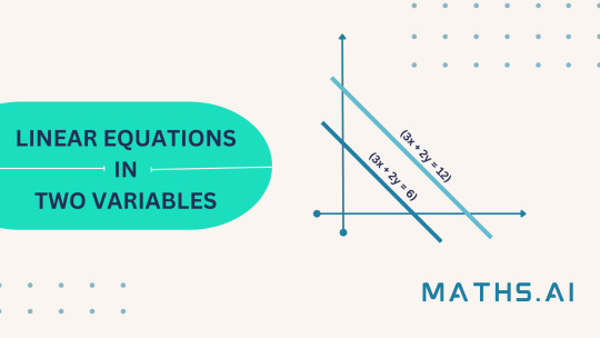
Solving linear equations with two variables is a fundamental skill in algebra that has real-world applications in various fields such as physics, economics, and engineering. These equations involve two unknowns and can be graphically represented as straight lines on a coordinate plane. In this article, we will explore two common methods for solving equations: the substitution method and the elimination method. Through step-by-step examples.

Method 1: Substitution Method

The substitution method involves solving one equation for one variable and substituting that expression into the other equation. Here's a detailed example to illustrate the process:

Example

Solve the following system of linear equations using the substitution method:

1. \(2x + y = 8\)

2. \(3x - 2y = 1\)

Step 1:

Solve one equation for one variable.

From equation (1), solve for \(y\):

\[y = 8 - 2x\]

Step 2:

Substitute the expression for \(y\) into the other equation.

Substitute \(y = 8 - 2x\) into equation (2):

\[3x - 2(8 - 2x) = 1\]

Step 3:

Solve for \(x\).

\[3x - 16 + 4x = 1\]

\[7x = 17\]

\[x = \frac{17}{7}\]

Step 4:

Substitute \(x\) value back to find \(y\).

Using the value of \(x\) in \(y = 8 - 2x\):

\[y = 8 - 2 \left(\frac{17}{7}\right) = \frac{3}{7}\]

So, the solution for the system of equations is \(x = \frac{17}{7}\) and \(y = \frac{3}{7}\).

Method 2: Elimination Method

The elimination method involves adding or subtracting the equations to eliminate one of the variables, making it easier to solve for the remaining variable. Let's solve the same system of equations using the elimination method:

Example

Solve the system of linear equations using the elimination method:

1. \(2x + y = 8\)

2. \(3x - 2y = 1\)

Step 1:

 Multiply the equations by suitable constants to make the coefficients of one of the variables equal.

Multiply equation (1) by 2 and equation (2) by 1 to make the coefficients of \(y\) equal:

\[2(2x + y) = 2 \cdot 8 \implies 4x + 2y = 16\]

\[3x - 2y = 1\]

Step 2:

 Add the equations to eliminate \(y\).

Add the two equations:

\[4x + 2y + 3x - 2y = 16 + 1\]

\[7x = 17\]

\[x = \frac{17}{7}\]

Step 3:

Substitute \(x\) value to find \(y\).

Using the value of \(x\) in equation (1):

\[2x + y = 8\]

\[2 \left(\frac{17}{7}\right) + y = 8\]

\[\frac{34}{7} + y = 8\]

\[y = \frac{3}{7}\]

The solution for the system of equations is \(x = \frac{17}{7}\) and \(y = \frac{3}{7}\).

.

Solving linear equations with two variables is a crucial skill in algebra, with applications extending to diverse fields. The substitution and elimination methods provide effective strategies for finding solutions, and through step-by-step examples, we've demonstrated how these methods work. With the advent of AI-based tools like Maths.ai, students now have access to personalized, interactive guidance that enhances their understanding and problem-solving abilities. As technology continues to evolve, the learning experience for mathematics is becoming more engaging and accessible, empowering students to excel in their studies and beyond.

[mathsai]

Finding the Area of a Triangle Step by Step 

Mathematics is often seen as a challenging subject, and one of the fundamental concepts in geometry. Students find difficulty while finding the area of a triangle. Whether you're a student grappling with geometry problems or someone looking to refresh their math skills, having a reliable Maths.ai can be immensely helpful. In this article, we will walk you through the step-by-step process of finding the area of a triangle.

Step 1: Understand the Formula

Before we dive into solving specific problems, it's essential to understand the formula used to calculate the area of a triangle. The formula is:

[ \text{Area} = \frac{1}{2} \times \text{Base} \times \text{Height} ]

Where:

"Base" refers to the length of the base of the triangle.

"Height" refers to the perpendicular distance from the base to the opposite vertex.

Step 2: Gather the Given Information

Let's start by considering a specific example problem: "Calculate the area of a triangle XYZ, where the base XY is 10 units long, and the height from vertex Z to base XY is 8 units."

In this case, we have:

Base (XY) = 10 units

Height (Z to XY) = 8 units

Step 3: Apply the Formula

Now that we have the formula and the given information, we can plug the values into the formula to calculate the area.

[ \text{Area} = \frac{1}{2} \times \text{Base} \times \text{Height} ]

Plugging in the values: [ \text{Area} = \frac{1}{2} \times 10 \times 8 ] [ \text{Area} = 5 \times 8 ] [ \text{Area} = 40 \text{ square units} ]

So, the area of triangle XYZ is 40 square units.

Step 4: Interpret the Result

Interpreting the result is equally important. In this case, the area of the triangle is 40 square units. This means that the region enclosed by the triangle XYZ covers an area of 40 square units.

Understanding how to calculate the area of a triangle is a fundamental skill in geometry. By following a step-by-step approach and utilizing Maths.ai, solving such problems becomes much more accessible and manageable. Remember to grasp the formula, gather the given information, apply the formula correctly, interpret the result, learning and mastering mathematical concepts can be an engaging and rewarding experience.

Whether you're a student aiming to ace your geometry class or an enthusiast looking to refresh your math skills, embracing AI technology like Maths.ai can provide you with the support and guidance needed to conquer maths problems with confidence. So, next time you encounter a triangle area calculation or any other maths challenge, don't hesitate to enlist the assistance of AI for a smoother learning journey.

[mathsai]

Solving Polynomials: A Step-by-Step Guide

Polynomials are mathematical expressions that involve variables raised to non-negative integer powers, combined with various coefficients and mathematical operations. Solving polynomials is a fundamental skill in algebra, and it forms the basis for solving a wide range of mathematical problems. In this article, we will explore the process of Solving Polynomials, step-by-step. We'll also provide a detailed example to illustrate the concepts.

Step 1: Understanding Polynomials

Before diving into solving polynomials, it's important to understand what they are. A polynomial is an algebraic expression consisting of terms, each of which has a coefficient and an exponent. For example, \(3x^2 - 5x + 2\) is a polynomial in the variable \(x\), where \(3\), \(-5\), and \(2\) are coefficients, and \(x^2\), \(x\), and the constant \(2\) are terms.

Step 2: Identifying the Polynomial Degree

The degree of a polynomial is determined by the highest exponent of the variable present in the polynomial. This is crucial because it helps us understand the behavior and characteristics of the polynomial. For instance, in the polynomial \(3x^2 - 5x + 2\), the highest exponent is \(2\), so the degree of the polynomial is \(2\), making it a quadratic polynomial.

Step 3: Factoring the Polynomial (if possible)

Factoring a polynomial involves breaking it down into simpler terms, which can often reveal its roots or solutions. The roots of a polynomial are the values of the variable that make the polynomial equal to zero. Let's consider an example to illustrate this process:

Example: Solve the quadratic polynomial \(x^2 - 5x + 6\) using factoring.

Solution:

1. Start with the polynomial: \(x^2 - 5x + 6\).

2. Try to factor the polynomial by finding two numbers whose product is the product of the coefficient of the quadratic term (\(1\)) and the constant term (\(6\)) and whose sum is the coefficient of the linear term (\(-5\)).

   - The numbers \(2\) and \(3\) satisfy these conditions: \(2 \times 3 = 6\) and \(2 + 3 = 5\).

3. Rewrite the middle term (\(-5x\)) using the factored numbers: \(x^2 - 2x - 3x + 6\).

4. Group the terms: \(x(x - 2) - 3(x - 2)\).

5. Factor out the common term \((x - 2)\): \((x - 2)(x - 3)\).

6. Set each factor equal to zero and solve for \(x\): \(x - 2 = 0\) or \(x - 3 = 0\).

7. Solve for \(x\): \(x = 2\) or \(x = 3\).

Step 4: Using the Quadratic Formula

In cases where factoring isn't possible or practical, the quadratic formula is a powerful tool for solving quadratic polynomials. The quadratic formula states that for a quadratic polynomial of the form \(ax^2 + bx + c = 0\), the solutions for \(x\) are given by:

\[x = \frac{-b \pm \sqrt{b^2 - 4ac}}{2a}\]

Where \(a\), \(b\), and \(c\) are the coefficients of the quadratic polynomial. Let's apply the quadratic formula to an example:

Example: Solve the quadratic polynomial \(2x^2 - 7x + 3\) using the quadratic formula.

Solution:

1. Start with the polynomial: \(2x^2 - 7x + 3\).

2. Identify the coefficients: \(a = 2\), \(b = -7\), and \(c = 3\).

3. Apply the quadratic formula: 

\[x = \frac{-(-7) \pm \sqrt{(-7)^2 - 4 \cdot 2 \cdot 3}}{2 \cdot 2}\]

4. Simplify the formula: 

\[x = \frac{7 \pm \sqrt{49 - 24}}{4}\]

\[x = \frac{7 \pm \sqrt{25}}{4}\]

5. Continue simplifying: 

\[x = \frac{7 \pm 5}{4}\]

6. Solve for both values of \(x\): 

\[x_1 = \frac{7 + 5}{4} = 3\]

\[x_2 = \frac{7 - 5}{4} = \frac{1}{2}\]

Step 5: Handling Higher-Degree Polynomials

For polynomials of degree higher than \(2\), factoring and the quadratic formula may not be sufficient. In such cases, we can use numerical methods like the Rational Root Theorem, synthetic division, or graphing to approximate solutions. Additionally, some higher-degree polynomials may have special properties that aid in finding solutions.

Solving polynomials is a crucial skill in algebra and lays the foundation for solving a variety of mathematical problems. By understanding the degree of the polynomial, factoring, using the quadratic formula, and employing other numerical methods, students can effectively find the solutions to polynomial equations. Whether the polynomial is linear, quadratic, or higher-degree, each type requires a unique approach to find its solutions. Armed with these techniques, students can confidently tackle a wide range of polynomial equations and gain a deeper appreciation for the beauty and complexity of mathematics.

In this article, we've explored the step-by-step process of solving polynomials. We've covered the fundamentals, demonstrated factoring and quadratic formula methods with examples, and touched on how to approach higher-degree polynomials. Through practice and understanding, students can master polynomial solving and develop essential problem-solving skills that extend to various mathematical and scientific disciplines. Remember, mathematics is not just about finding answers; it's about the journey of exploration, discovery, and critical thinking. Use maths.ai to unlock your mathematical journey.

[mathsai]

A Comprehensive Guide of Solving Probability:

Probability, a fundamental concept in mathematics, permeates various aspects of our lives. From predicting the outcome of a coin toss to making informed decisions in uncertain situations, probability plays a crucial role. In this guide, we will delve into the world of probability, exploring its definition, applications, and two key methods for solving probability problems. Whether you're a student seeking a deeper understanding of this topic or someone interested in brushing up on their probability skills, this article aims to provide clarity and guidance.

Probability: A Brief Overview

Probability is the measure of the likelihood that an event will occur. It is expressed as a number between 0 and 1, where 0 represents impossibility, 1 signifies certainty, and values in between reflect varying degrees of likelihood. In mathematical terms, the probability of an event A is denoted as P(A).

Applications of Probability

Probability theory finds applications in numerous fields, such as statistics, finance, science, and even artificial intelligence. It allows us to make informed predictions, assess risks, and analyze data patterns. For instance, probability is used in weather forecasting, stock market analysis, and medical research to model uncertain outcomes.

Two Methods of Solving Probability Problem

Classical Probability

Classical probability, also known as "priori" probability, is based on equally likely outcomes. This method is applicable when all possible outcomes of an experiment are equally likely, and it's commonly used in scenarios like coin tosses or rolling fair dice.

Example: Coin Toss

Imagine a fair coin toss. There are two possible outcomes: heads (H) or tails (T). Since the coin is fair, each outcome has an equal probability of 0.5. To calculate the probability of getting heads, we use the formula:

[ P(H) = \frac{\text{Number of favorable outcomes}}{\text{Total number of outcomes}} = \frac{1}{2} = 0.5. ]

Empirical Probability

Empirical probability, also called "experimental" or "observed" probability, is based on observations from actual experiments or real-world data. It involves counting the occurrences of a specific event and dividing it by the total number of trials.

Example: Rolling a Die

Consider rolling a standard six-sided die. To calculate the probability of rolling a 3, you could conduct a series of rolls and record the results. If you roll the die 100 times and get 15 threes, the empirical probability of rolling a 3 is:

[ P(\text{Rolling a 3}) = \frac{\text{Number of times 3 is rolled}}{\text{Total number of trials}} = \frac{15}{100} = 0.15. ]

Card Games as a Probability  Playground

Card games provide an excellent platform for understanding probability. A standard deck of playing cards contains 52 cards, divided into four suits: hearts, diamonds, clubs, and spades. Each suit has 13 ranks: Ace through 10, followed by Jack, Queen, and King. Let's dive into some examples to illustrate the concepts.

Example 1: Drawing a Specific CardExample 1: Drawing a Specific Card

Suppose we want to find the probability of drawing an Ace from a standard deck of 52 cards.

Step 1: Determine the Total Possible Outcomes

In a deck of 52 cards, there are 4 Aces (one in each suit). Therefore, the total possible outcomes are 52 (the total number of cards in the deck).

Step 2: Determine the Favorable Outcomes

Since there are 4 Aces in the deck, the number of favorable outcomes is 4.

Step 3: Calculate the Probability

The probability of drawing an Ace is calculated using the formula:

\[ \text{Probability} = \frac{\text{Number of Favorable Outcomes}}{\text{Total Possible Outcomes}} = \frac{4}{52} = \frac{1}{13} \approx 0.0769 \]

Example 2: Drawing Cards of a Certain Suit

Now let's consider the probability of drawing a heart from the deck.

Step 1: Total Possible Outcomes

In a deck of 52 cards, there are 13 hearts.

Step 2: Favorable Outcomes

The number of hearts in the deck is 13.

Step 3: Probability Calculation

\[ \text{Probability of drawing a heart} = \frac{\text{Number of Hearts}}{\text{Total Number of Cards}} = \frac{13}{52} = \frac{1}{4} = 0.25 \]

Probability is an essential concept with diverse applications in various fields, offering insights into uncertain situations and enabling informed decision-making. In this guide, we explored the definitions and applications of probability, focusing on two fundamental methods of solving probability problems: classical and empirical probability. We also witnessed how Maths.ai, can assist students in solving probability problems step by step, enhancing their understanding and confidence in handling such challenges.

As you continue your journey into the fascinating world of mathematics, remember that probability is not just about numbers; it's about gaining a deeper insight into the inherent uncertainty of the world around us. Through consistent practice, problem-solving, and utilizing AI-driven resources like Maths.ai, you can master probability and develop valuable skills applicable to a wide range of disciplines.

[mathsai]

Mathematical Reasoning: A Complete Guide

Mathematical Reasoning is the foundation of problem-solving and critical thinking in mathematics. It involves the ability to analyze, deduce, and draw conclusions from mathematical concepts, principles, and relationships. In this guide, we will explore the key aspects of mathematical reasoning, provide examples to illustrate its application, and discuss effective methods for developing strong mathematical reasoning skills.

Key Aspects of Mathematical Reasoning

Logical Deduction:

Mathematical reasoning involves using logical deduction to arrive at conclusions based on given information or premises. It requires the ability to follow a chain of reasoning step by step, ensuring that each step is based on sound logic.

Pattern Recognition:

Recognizing patterns and relationships is crucial for mathematical reasoning. Identifying trends and regularities helps in making conjectures and predictions, and aids in solving problems efficiently.

Abstraction:

Abstraction involves generalizing specific cases into broader concepts. It allows us to work with generalized properties rather than specific instances, making problem-solving more versatile.

Inductive and Deductive Reasoning:

Inductive reasoning involves making generalizations based on a set of specific observations, while deductive reasoning uses established principles to draw specific conclusions. Both are important for mathematical reasoning.

Counter examples:

Counterexamples are instances that disprove a conjecture or statement. Considering counterexamples is crucial to test the validity of a mathematical claim.

Proofs:

Mathematical proofs are rigorous arguments that establish the truth of a statement or proposition. Constructing and understanding proofs is a fundamental aspect of mathematical reasoning.

Examples Illustrating Mathematical Reasoning

Example: Fibonacci Numbers

Consider the Fibonacci sequence: 0, 1, 1, 2, 3, 5, 8, ..

By observing the pattern, we notice that each term is the sum of the previous two terms. This pattern leads to a conjecture: the nth term is the sum of the (n-1)th and (n-2)th terms. We can prove this by mathematical induction.

Example: Prime Numbers

 Prime numbers are positive integers greater than 1 that have no divisors other than 1 and themselves. By using deductive reasoning, we can prove that there are infinitely many prime numbers. Suppose there are only finitely many primes. We can then consider the number obtained by multiplying all existing primes and adding 1. This number is either prime itself (contradicting the assumption) or has a prime factor that is not in our list, leading to a contradiction.

Example: Pythagorean Theorem

 The Pythagorean Theorem states that in a right-angled triangle, the square of the length of the hypotenuse is equal to the sum of the squares of the other two sides.

Mathematical Reasoning: One way to prove this theorem is using geometric reasoning. Consider a square with side lengths a + b, where a and b are the lengths of the triangle's legs. The square can be divided into smaller squares and

rearranged to show that the area of the large square is equal to the sum of the areas of the two smaller squares.

Methods for Developing Strong Mathematical Reasoning Skills

Practice Problem-Solving:

Regularly solve a variety of mathematical problems. Start with simpler problems and gradually work your way up to more complex ones. This will help you develop pattern recognition and logical deduction skills.

Analyze Proofs:

Study different types of mathematical proofs. Understand the structure of a proof, from the assumptions to the conclusion. This will enhance your ability to construct rigorous arguments.

Explore Counterexamples:

When encountering a new conjecture, try to find counterexamples that might disprove it. This practice will help you refine your reasoning skills and think critically about mathematical statements.

Work Collaboratively:

Discuss mathematical problems and concepts with peers or mentors. Explaining your reasoning to others and listening to their perspectives can provide new insights and broaden your understanding.

Engage with Mathematical Literature:

Read mathematical books, papers, and articles. Exposing yourself to various mathematical ideas and approaches will expand your toolkit for reasoning.

Participate in Math Competitions:

Joining math competitions or problem-solving clubs can challenge you to think creatively and critically under time constraints.

Mathematical Reasoning is a fundamental skill that underlies all branches of mathematics. It involves logical deduction, pattern recognition, abstraction, and the ability to construct and understand proofs. By engaging with examples and following effective methods, you can develop strong mathematical reasoning skills that will serve you well in both academic and real-world problem-solving scenarios. Regular practice, thoughtful analysis, and a curious mindset are key to mastering this essential skill. Visit maths.ai to help in solving maths problems.