my-naomi-blog

[my-naomi-blog]

Week 4

INPUT 

import pandas import numpy import seaborn import matplotlib.pyplot as plt # any additional libraries would be imported here

mydata = pandas.read_csv('prostate_1.csv', low_memory=False)

# subset variables in new data frame, sub1 sub1=mydata[['AgeF','PSA', 'Cancer Volume']]

a = sub1.head print(a)

#new PSA variable, categorical 1 through 2 def PSA (row):   if row['PSA'] < 4 :      return 1   if row['PSA'] > 4 :      return 2 sub1['PSA'] = sub1.apply (lambda row: PSA (row),axis=1)

a = sub1.head print(a)

#new Age variable, categorical 1 through 2 def Age (row):   if row['AgeF']== '41-50':      return 1   if row['AgeF'] == '51-60' :      return 2   if row['AgeF'] == '61-70' :      return 3   if row['AgeF'] == '71-80' :      return 4 sub1['Age'] = sub1.apply (lambda row: Age (row),axis=1)

a = sub1.head print(a)

#new Cancer_Volume variable, categorical 1 through 4 def Cancer_Volume(row):   if row['Cancer Volume'] < 11:      return 1   if row['Cancer Volume'] >11 and row['Cancer Volume'] < 21 :      return 2   if row['Cancer Volume'] >21 and row['Cancer Volume'] <31 :      return 3   if row['Cancer Volume'] >31:      return 4 sub1['Cancer_Volume'] = sub1.apply (lambda row: Cancer_Volume(row),axis=1)

a = sub1.head print(a)

#univariate bar graph for categorical variables for PSA level # First hange format from numeric to categorical sub1["PSA"] = sub1["PSA"].astype('category')

seaborn.countplot(x="PSA", data=sub1) plt.xlabel('PSA level') plt.title('PSA level Among Adult men who visited the university medical center in the Prostate cancer Study')

#univariate bar graph for categorical variables for Age groups # First hange format from numeric to categorical sub1["AgeF"] = sub1["AgeF"].astype('category')

seaborn.countplot(x="AgeF", data=sub1) plt.xlabel('AgeF') plt.title('Age groups Among Adult men who visited the university medical center in the Prostate cancer Study')

#univariate bar graph for categorical variables for Cancer Volume # First hange format from numeric to categorical sub1["Cancer_Volume"] = sub1["Cancer_Volume"].astype('category')

seaborn.countplot(x="Cancer_Volume", data=sub1) plt.xlabel('Cancer_Volume') plt.title('Cancer Volume Among Adult men who visited the university medical center in the Prostate cancer Study')

# standard deviation and other descriptive statistics for quantitative variables

print ('PSA level') desc2 = sub1['PSA'].describe() print (desc2)

c1= sub1.groupby('PSA').size() print (c1)

print ('mode PSA level') mode1 = sub1['PSA'].mode() print (mode1)

c1= sub1.groupby('PSA').size() print (c1)

p1 = sub1.groupby('PSA').size() * 100 / len(mydata) print (p1)

# standard deviation and other descriptive statistics for quantitative variables

print ('Age') desc2 = sub1['AgeF'].describe() print (desc2)

c2= sub1.groupby('AgeF').size() print (c2)

print ('mode of Age') mode1 = sub1['AgeF'].mode() print (mode1)

p2 = sub1.groupby('AgeF').size() * 100 / len(mydata) print (p2)

print ('Cancer Volume') desc2 = sub1['Cancer_Volume'].describe() print (desc2)

c2= sub1.groupby('Cancer_Volume').size() print (c2)

print ('Mode of Cancer Volume') mode1 = sub1['Cancer_Volume'].mode() print (mode1)

# bivariate bar graph C->Q seaborn.factorplot(x='AgeF', y='PSA', data=mydata, kind="bar", ci=None) plt.xlabel('Age') plt.ylabel('PSA level')

OUTPUT

<bound method NDFrame.head of      AgeF      PSA  Cancer Volume 0   41-50    0.651         0.5599 1   51-60    0.852         0.3716 2   71-80    0.852         0.6005 3   51-60    0.852         0.3012 4   61-70    1.448         2.1170 ..    ...      ...            ... 92  61-70   80.640        16.9455 93  41-50  107.770        45.6042 94  51-60  170.716        18.3568 95  61-70  239.847        17.8143 96  61-70  265.072        32.1367

[97 rows x 3 columns]> <bound method NDFrame.head of      AgeF  PSA  Cancer Volume 0   41-50    1         0.5599 1   51-60    1         0.3716 2   71-80    1         0.6005 3   51-60    1         0.3012 4   61-70    1         2.1170 ..    ...  ...            ... 92  61-70    2        16.9455 93  41-50    2        45.6042 94  51-60    2        18.3568 95  61-70    2        17.8143 96  61-70    2        32.1367

[97 rows x 3 columns]> <bound method NDFrame.head of      AgeF  PSA  Cancer Volume  Age 0   41-50    1         0.5599    1 1   51-60    1         0.3716    2 2   71-80    1         0.6005    4 3   51-60    1         0.3012    2 4   61-70    1         2.1170    3 ..    ...  ...            ...  ... 92  61-70    2        16.9455    3 93  41-50    2        45.6042    1 94  51-60    2        18.3568    2 95  61-70    2        17.8143    3 96  61-70    2        32.1367    3

[97 rows x 4 columns]> <bound method NDFrame.head of      AgeF  PSA  Cancer Volume  Age  Cancer_Volume 0   41-50    1         0.5599    1              1 1   51-60    1         0.3716    2              1 2   71-80    1         0.6005    4              1 3   51-60    1         0.3012    2              1 4   61-70    1         2.1170    3              1 ..    ...  ...            ...  ...            ... 92  61-70    2        16.9455    3              2 93  41-50    2        45.6042    1              4 94  51-60    2        18.3568    2              2 95  61-70    2        17.8143    3              2 96  61-70    2        32.1367    3              4

[97 rows x 5 columns]> PSA level count     97 unique     2 top        2 freq      83 Name: PSA, dtype: int64 PSA 1    14 2    83 dtype: int64 mode PSA level 0    2 Name: PSA, dtype: category Categories (2, int64): [1, 2] PSA 1    14 2    83 dtype: int64 PSA 1    14.43299 2    85.56701 dtype: float64 Age count        97 unique        4 top       61-70 freq         59 Name: AgeF, dtype: object AgeF 41-50     8 51-60    17 61-70    59 71-80    13 dtype: int64 mode of Age 0    61-70 Name: AgeF, dtype: category Categories (4, object): [41-50, 51-60, 61-70, 71-80] AgeF 41-50     8.247423 51-60    17.525773 61-70    60.824742 71-80    13.402062 dtype: float64 Cancer Volume count     97 unique     4 top        1 freq      75 Name: Cancer_Volume, dtype: int64 Cancer_Volume 1    75 2    16 3     4 4     2 dtype: int64 Mode of Cancer Volume 0    1 Name: Cancer_Volume, dtype: category Categories (4, int64): [1, 2, 3, 4]

The univariate graph of PSA level:

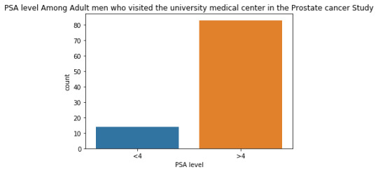
This graph is unimodal, with its highest peak at the�� category of >4 PSA level . It seems to be skewed to the left as there are higher frequencies in higher category(>4) than the lower category.

The univariate graph of Age groups:

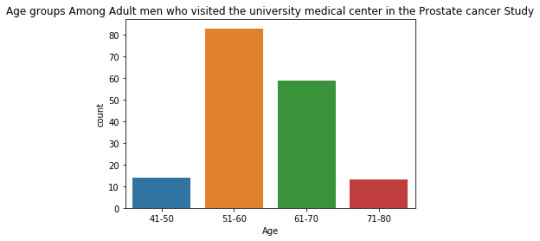
This graph is unimodal, with its highest peak at 51 to 60 age group. It seems to be skewed to the right as there are higher frequencies in the lower age ranges from 51 to 60.

The univariate graph of Cancer Volume:

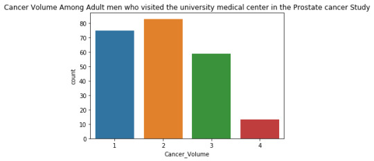
This graph is unimodal, with its highest peak at the  category of 2 (11-20) . It seems to be skewed to the right as there are higher frequencies in lower categories than the higher categories.

The graph above plots the Cancer Volume of the adult men  to the adult men corresponding Age groups. We can see that the bar chat does not show a clear relationship/trend between the two variables.

[my-naomi-blog]

Week 3

import pandas

import numpy

# any additional libraries would be imported here

mydata = pandas.read_csv('prostate_1.csv', low_memory=False)

# subset variables in new data frame, sub1

sub1=mydata[['AgeF','PSA', 'Cancer Volume']]

a = sub1.head

print(a)

#new PSA variable, categorical 1 through 2

def PSA (row):

   if row['PSA'] < 4 :

      return 1

   if row['PSA'] > 4 :

      return 2

sub1['PSA'] = sub1.apply (lambda row: PSA (row),axis=1)

a = sub1.head 

print(a)

#new Age variable, categorical 1 through 2

def Age (row):

   if row['AgeF']== '41-50':

      return 1

   if row['AgeF'] == '51-60' :

      return 2

   if row['AgeF'] == '61-70' :

      return 3

   if row['AgeF'] == '71-80' :

      return 4

sub1['Age'] = sub1.apply (lambda row: Age (row),axis=1)

a = sub1.head 

print(a)

#new Cancer_Volume variable, categorical 1 through 4

def Cancer_Volume(row):

   if row['Cancer Volume'] < 11:

      return 1

   if row['Cancer Volume'] >11 and row['Cancer Volume'] < 21 :

      return 2

   if row['Cancer Volume'] >21 and row['Cancer Volume'] <31 :

      return 3

   if row['Cancer Volume'] >31:

      return 4

sub1['Cancer_Volume'] = sub1.apply (lambda row: Cancer_Volume(row),axis=1)

a = sub1.head 

print(a)

#frequency distributions for primary and secondary ethinciity variables

print( 'counts for PSA level')

c10 = sub1['PSA'].value_counts(sort=False)

print(c10)

print( 'percentages for PSA level')

p10 = sub1['PSA'].value_counts(sort=False, normalize=True)

print (p10)

print('counts for Age')

c11 = sub1['Age'].value_counts(sort=False)

print(c11)

print( 'percentages for Age')

p11= sub1['Age'].value_counts(sort=False, normalize=True)

print (p11)

print( 'counts for Cancer Volume')

c12 = sub1['Cancer_Volume'].value_counts(sort=False)

print(c12)

print( 'percentages for Cancer Volume')

p12 = sub1['Cancer_Volume'].value_counts(sort=False, normalize=True)

print (p12)

Output

runfile('C:/Users/NAOMI/Downloads/Documents/Cousera/Data Visualization/week 3/Assignment 3 new.py', wdir='C:/Users/NAOMI/Downloads/Documents/Cousera/Data Visualization/week 3') <bound method NDFrame.head of      AgeF      PSA  Cancer Volume 0   41-50    0.651         0.5599 1   51-60    0.852         0.3716 2   71-80    0.852         0.6005 3   51-60    0.852         0.3012 4   61-70    1.448         2.1170 ..    ...      ...            ... 92  61-70   80.640        16.9455 93  41-50  107.770        45.6042 94  51-60  170.716        18.3568 95  61-70  239.847        17.8143 96  61-70  265.072        32.1367

[97 rows x 3 columns]> <bound method NDFrame.head of      AgeF  PSA  Cancer Volume 0   41-50    1         0.5599 1   51-60    1         0.3716 2   71-80    1         0.6005 3   51-60    1         0.3012 4   61-70    1         2.1170 ..    ...  ...            ... 92  61-70    2        16.9455 93  41-50    2        45.6042 94  51-60    2        18.3568 95  61-70    2        17.8143 96  61-70    2        32.1367

[97 rows x 3 columns]> <bound method NDFrame.head of      AgeF  PSA  Cancer Volume  Age 0   41-50    1         0.5599    1 1   51-60    1         0.3716    2 2   71-80    1         0.6005    4 3   51-60    1         0.3012    2 4   61-70    1         2.1170    3 ..    ...  ...            ...  ... 92  61-70    2        16.9455    3 93  41-50    2        45.6042    1 94  51-60    2        18.3568    2 95  61-70    2        17.8143    3 96  61-70    2        32.1367    3

[97 rows x 4 columns]> <bound method NDFrame.head of      AgeF  PSA  Cancer Volume  Age  Cancer_Volume 0   41-50    1         0.5599    1              1 1   51-60    1         0.3716    2              1 2   71-80    1         0.6005    4              1 3   51-60    1         0.3012    2              1 4   61-70    1         2.1170    3              1 ..    ...  ...            ...  ...            ... 92  61-70    2        16.9455    3              2 93  41-50    2        45.6042    1              4 94  51-60    2        18.3568    2              2 95  61-70    2        17.8143    3              2 96  61-70    2        32.1367    3              4

[97 rows x 5 columns]> counts for PSA level 1    14 2    83 Name: PSA, dtype: int64 percentages for PSA level 1    0.14433 2    0.85567 Name: PSA, dtype: float64 counts for Age 1     8 2    17 3    59 4    13 Name: Age, dtype: int64 percentages for Age 1    0.082474 2    0.175258 3    0.608247 4    0.134021 Name: Age, dtype: float64 counts for Cancer Volume 1    75 2    16 3     4 4     2 Name: Cancer_Volume, dtype: int64 percentages for Cancer Volume 1    0.773196 2    0.164948 3    0.041237 4    0.020619 Name: Cancer_Volume, dtype: float64

I created new data with  three variables: AgeF, PSA and Cancer Volume. The were no missing data set in my data. For Age, the most commonly endorsed is 3 (60.8%) , meaning  more than half of the  men who went for the checkup are from the age 61-70 years. For PSA, 2 (85.57%) has the highest percentage, meaning the PSA which is greater than 4 has the highest frequency of 83. For Cancer Volume, 1 ( 77.32% ) has the highest percentage among the others which means the Cancer Volume less than 10 has  the highest frequency of 75 with 77.32%.

[my-naomi-blog]

My program (code)

import pandas import numpy

mydata = pandas.read_csv("prostate_1.csv", low_memory = False)

print(len(mydata))  #prints out number of observations (row) print(len(mydata.columns))  #prints out number of columns(variables)

mydata["Age"]= mydata["AgeF"] mydata["PSA"]= mydata["PSAF"]

#counts and percentages (i.e. frequency distributions) for each variable print("count for Age groups") count1 = mydata['Age'].value_counts(sort=False) print (count1)

print("percentages for Age groups") p1 = mydata['Age'].value_counts(sort=False, normalize=True) print (p1)

print("count for PSA level")  #PSA was grouped into 2 that is <4 and >4 count2 = mydata["PSA"].value_counts(sort=False) print(count2)

print("percentages for PSA level ") p2 = mydata["PSA"].value_counts(sort=False, normalize=True) print(p2)

print("count for Weight of cancer in gm") count4 = mydata["Weight"].value_counts(sort=False) print(count4)

print("percentages for Weight of cancer in gm ") p4 = mydata["Weight"].value_counts(sort=False, normalize = True) print(p4)

# freqeuncy disributions using the 'bygroup' function cot1= mydata.groupby('Age').size() print(cot1)

pot1 = mydata.groupby('Age').size() * 100 / len(mydata) print(pot1)

cot2= mydata.groupby('PSA').size() print(cot2)

pot2 = mydata.groupby('PSA').size() * 100 / len(mydata) print (pot2)

cot4= mydata.groupby('Weight').size() print (cot4)

pot4 = mydata.groupby('Weight').size() * 100 / len(mydata) print (pot4)

#upper-case all DataFrame column names - place afer code for loading data aboave mydata.columns = map(str.upper, mydata.columns)

# bug fix for display formats to avoid run time errors - put after code for loading data above pandas.set_option('display.float_format', lambda x:'%f'%x)

Output

97

12

count for Age group

51-60    17

41-50     8

71-80    13

61-70    59

Name: Age, dtype: int64

percentages for Age groups

51-60   0.175258

41-50   0.082474

71-80   0.134021

61-70   0.608247

Name: Age, dtype: float64

count for PSA level

>4    83

<4    14

Name: PSA, dtype: int64

percentages for PSA level 

>4   0.855670

<4   0.144330

Name: PSA, dtype: float64

count for Weight

31.500000    1

29.964000    1

10.697000    1

21.542000    1

59.740000    2

            ..

23.104000    1

22.646000    1

45.604000    1

39.646000    2

42.948000    1

Name: Weight, Length: 77, dtype: int64

percentages for Weight

31.500000   0.010309

29.964000   0.010309

10.697000   0.010309

21.542000   0.010309

59.740000   0.020619

  23.104000   0.010309

22.646000   0.010309

45.604000   0.010309

39.646000   0.020619

42.948000   0.010309

Name: Weight, Length: 77, dtype: float64

Age

41-50     8

51-60    17

61-70    59

71-80    13

dtype: int64

Age

41-50    8.247423

51-60   17.525773

61-70   60.824742

71-80   13.402062

dtype: float64

PSA

<4    14

>4    83

dtype: int64

PSA

<4   14.432990

>4   85.567010

dtype: float64

Weight

10.697000     1

14.732000     1

15.959000     1

17.637000     1

20.086000     1

             ..

83.931000     1

91.836000     1

112.168000    1

119.104000    1

450.339000    1

Length: 77, dtype: int64

Weight

10.697000    1.030928

14.732000    1.030928

15.959000    1.030928

17.637000    1.030928

20.086000    1.030928

  83.931000    1.030928

91.836000    1.030928

112.168000   1.030928

119.104000   1.030928

450.339000   1.030928

Length: 77, dtype: float64

runfile('C:/Users/NAOMI/Documents/Anaconda/Anaconda work/Assignment.py', wdir='C:/Users/NAOMI/Documents/Anaconda/Anaconda work')

97

12

count for Age group

51-60    17

41-50     8

71-80    13

61-70    59

Name: Age, dtype: int64

percentages for Age groups

51-60   0.175258

41-50   0.082474

71-80   0.134021

61-70   0.608247

Name: Age, dtype: float64

count for PSA level

>4    83

<4    14

Name: PSA, dtype: int64

percentages for PSA level 

>4   0.855670

<4   0.144330

Name: PSA, dtype: float64

count for Weight

31.500000    1

29.964000    1

10.697000    1

21.542000    1

59.740000    2

            ..

23.104000    1

22.646000    1

45.604000    1

39.646000    2

42.948000    1

Name: Weight, Length: 77, dtype: int64

percentages for Weight

31.500000   0.010309

29.964000   0.010309

10.697000   0.010309

21.542000   0.010309

59.740000   0.020619

  23.104000   0.010309

22.646000   0.010309

45.604000   0.010309

39.646000   0.020619

42.948000   0.010309

Name: Weight, Length: 77, dtype: float64

Age

41-50     8

51-60    17

61-70    59

71-80    13

dtype: int64

Age

41-50    8.247423

51-60   17.525773

61-70   60.824742

71-80   13.402062

dtype: float64

PSA

<4    14

>4    83

dtype: int64

PSA

<4   14.432990

>4   85.567010

dtype: float64

Weight

10.697000     1

14.732000     1

15.959000     1

17.637000     1

20.086000     1

             ..

83.931000     1

91.836000     1

112.168000    1

119.104000    1

450.339000    1

Length: 77, dtype: int64

Weight

10.697000    1.030928

14.732000    1.030928

15.959000    1.030928

17.637000    1.030928

20.086000    1.030928

  83.931000    1.030928

91.836000    1.030928

112.168000   1.030928

119.104000   1.030928

450.339000   1.030928

Length: 77, dtype: float64

This result shows that the adult from age 61-70 has the highest frequency with 61% followed by 51-60. The PSA level was grouped into two under <4 and >4. The PSA level with >4 has the highest frequency with 86%.

[my-naomi-blog]

Regression Analysis of the factors affecting high grade prostate cancer in patients.

I have decided that I am particularly interested in high grade prostate cancer and this my own data set. I have included all the factors which I think are the main causes of high grade prostate cancer. Examples of factors include age of patients, prostate weight.

   Research Questions

1. Does age positively affect high grade prostate cancer?

2. Is there a high correlation between high grade prostate cancer and the various factors?

 Topic of Interest

Regression Analysis of the factors affecting high grade prostate cancer in patients.

 Second (Related) Topic of Interest

Correlation among variables stated in our codebook.

Correlation is the measure of the strength of the linear relationship among, usually, continuous random variables. Correlation is always between -1 and +1. Values closer to -1 and +1 indicate high negative and high positive correlation respectively i.e. a strong positive or negative association. Correlation values closer to zero indicates weak relationship among the variables of interest.

 Literature Review

Prostate cancer is the second most common diagnosed cancer and the fourth leading cause of cancer death in men worldwide (WCRF 2019). Physicians use rectal examination and prostate-specific antigen (PSA) concentration in blood to detect prostate cancer (Catalona et al. 1997, Heindenreich et al. 2014), the former is not welcome because of psychological implications and the latter could yield false-positive or false-negative results.

The severity of prostate cancer and survival probability of diagnosed patients can be estimated with the Gleason Score (Stark et al. 2009), but its accuracy and precision depend on multiple biopsies (PCEC 2019), another invasive and traumatic method. Other variables that might be associated to Gleason Score that can be obtained by less invasive methods and may be used to predict prostate cancer risk, for instance: prostate weight, benign prostate hyperplasia and seminal vesicle invasion, can be effectively detected and measured using ultrasonography (Kilic et al. 2014, Soylu et al. 2013).

The use of morphological and physiological parameters measured by noninvasive methods to predict the presence of high-grade prostate cancer remains unstudied. In this work we used seven morphological and physiological variables that can be measured in blood samples and ultrasonography to estimate the probability of presence of high-grade prostate cancer and therefore reduced the psychological impact of invasive diagnostic methods. It was recognized that age was the predominant factor affecting high grade prostate cancer (Naveda et al. 2019).

 Hypothesis

Age is the principal determinant of high grade cancer. The probability of presence of high-grade prostate cancer increases as a person ages.

  CodeBook

Adapted in part from: Hastie, T. J.; R. J. Tibshirani; and J. Friedman. The Elements of Statistical Learning: Data Mining. Inference. And Prediction. New York: Springer-Verlag, 2001.

 Applied Linear Regression Models edition 5 Kutner et al.