#data management and visualization

[drt-coursera]

Data Management and VisualizationModule 4 - Python My1stProgram

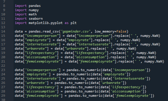
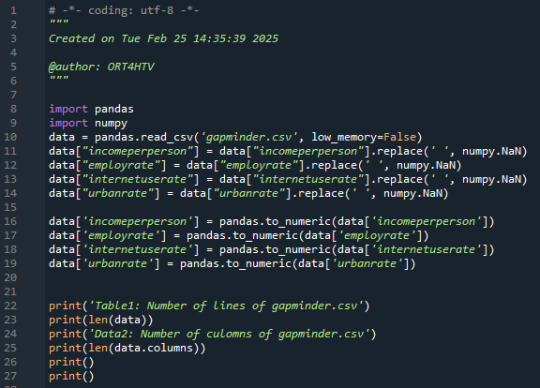
Basic data manipulation for converting ' ' to Nan:

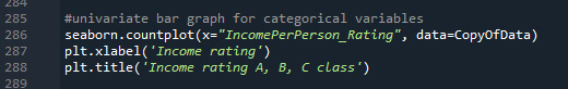
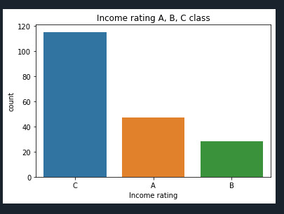
Bar graph for categorical variables:

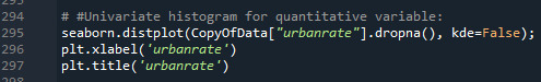
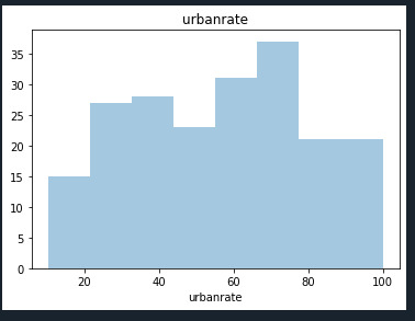
histogram for quantitative variable:

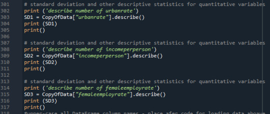
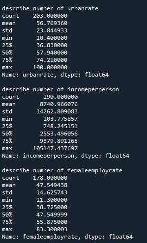
standard deviation and other descriptive statistics for quantitative variables:

Scatteerplot is created to show data desribed below:

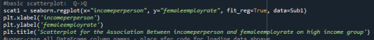
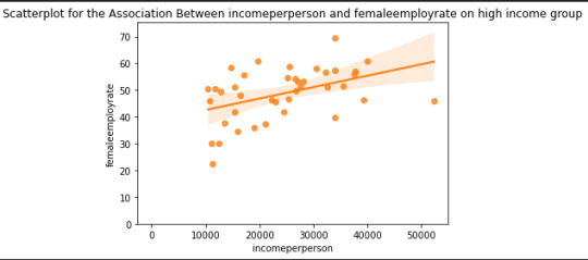
The basic hypothesis is disproved here as it is clearly visible the more the income the most the female employ rate is.

[mayaelsawy]

My Research Project Has Started

I have chosen to work with data from the World Bank Enterprise Surveys (WBES), which collect detailed information from firms across various countries about their business environment, performance, and practices. After reviewing the available datasets, I am particularly interested in exploring the relationship between green logistics practices and operating costs.

The motivation for this topic stems from growing interest in sustainable business practices, especially within supply chains, and how environmental initiatives such as green transportation, reduced packaging, or energy-efficient warehousing can impact financial performance. This issue is directly aligned with SDG 12 (Responsible Consumption and Production) and SDG 13 (Climate Action).

Main Research Question:

Is the adoption of green logistics practices associated with reduced operating costs?

Secondary Research Questions:

Do firms with environmental policies targeting logistics report lower transportation or utility costs?

Does the size or sector of a business moderate the relationship between green logistics adoption and cost outcomes?

Are firms that implement green practices more likely to report innovation or investment in sustainability?

Variables and Codes:

1. Green Logistics Practices

a. Environmental Management System (EMS)

Variable Definition: Whether the business has a certified environmental management system (e.g., ISO 14001).

Potential Codes:

1: Yes

0: No

b. Packaging Reduction

Variable Definition: Whether the firm reports taking action to reduce packaging waste for environmental reasons.

Potential Codes:

1: Yes

0: No

c. Energy Efficiency in Logistics

Variable Definition: Measures adoption of energy-saving strategies in logistics or warehouse operations.

Potential Codes:

1: Yes

0: No

2. Operating Costs

a. Overall Operating Costs

Variable Definition: Total operational costs as a percentage of revenue.

Potential Codes: Continuous variable (0–100)

b. Transportation Costs

Variable Definition: Proportion of costs spent on logistics and transportation.

Potential Codes: Continuous variable (0–100)

c. Utility Costs

Variable Definition: Proportion of business costs related to electricity, water, and fuel.

Potential Codes: Continuous variable (0–100)

3. Control Variables (Firm Characteristics)

a. Firm Size

Variable Definition: Number of employees.

Potential Codes:

1: Small (<20 employees)

2: Medium (20–99 employees)

3: Large (100+ employees)

b. Industry Sector

Variable Definition: Sector of business operations.

Potential Codes:

1: Manufacturing

2: Retail

3: Services

4: Other

c. Country or Region

Variable Definition: Geographic location of the firm.

Potential Codes: Country names or regions (e.g., Latin America, East Asia)

Literature Review Summary:

There is growing evidence linking sustainability practices with operational efficiency. A few key studies include:

Rao & Holt (2005) : Found that environmentally conscious supply chains can enhance performance by reducing waste and cutting costs.

Chiarini & Vagnoni (2017) : Demonstrated that firms with ISO 14001 certification observed long-term savings in energy and logistics costs.

Ahi & Searcy (2015) : Emphasized the dual benefit of environmental and financial performance from green logistics adoption.

Zhu, Geng & Sarkis (2013) : Found that firms in developing economies that implemented green supply chain practices reported improved cost control.

These studies support the idea that green practices are not just environmentally beneficial, but can also enhance cost efficiency and resilience in the supply chain.

Hypothesis:

Firms that adopt green logistics practices will report lower operating costs, particularly in transportation and utility expenses, compared to firms that do not implement such practices.

This relationship may vary by firm size or industry sector but is expected to hold generally across contexts.

[youngtigercheesecake]

Week 4

Creating graphs for your data code

import pandas import numpy import pandas as pd import seaborn import matplotlib.pyplot as plt

data = pd.read_csv('gapminder_pds.csv', low_memory=False)

bindata = data.copy()

convert variables to numeric format using convert_objects function

data['internetuserate'] = pd.to_numeric(data['internetuserate'], errors='coerce') bindata['internetuserate'] = pd.cut(data.internetuserate, 10)

data['incomeperperson'] = pd.to_numeric(data['incomeperperson'], errors='coerce') bindata['incomeperperson'] = pd.cut(data.incomeperperson, 10)

data['employrate'] = pd.to_numeric(data['employrate'], errors='coerce') bindata['employrate'] = pd.cut(data.employrate, 10)

data['femaleemployrate'] = pd.to_numeric(data['femaleemployrate'], errors='coerce') bindata['femaleemployrate'] = pd.cut(data.femaleemployrate, 10)

data['polityscore'] = pd.to_numeric(data['polityscore'], errors='coerce') bindata['polityscore'] = data['polityscore'] sub2 = bindata.copy()

Scatterplot for the Association Between Employment rate and lifeexpectancy

scat1 = seaborn.regplot(x="internetuserate", y="incomeperperson", fit_reg=False, data=data) plt.xlabel('Internet use rate') plt.ylabel('Income per person') plt.title('Scatterplot for the Association Between Internet use rate and Income per person')

This scatterplot show the relationship and seems to be exponential.

Univariate histogram for quantitative variable:

seaborn.distplot(data["incomeperperson"].dropna(), kde=False); plt.xlabel('Income per person')

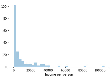
The graph is highly right skewed. Incomes are small for most of the world and the wealthy tail is quite long.

Univariate histogram for quantitative variable:

seaborn.distplot(data["employrate"].dropna(), kde=False); plt.xlabel('Employ rate')

Summary

It looks like there are associations between Internet use rate and income per person going up with internet use rate and going up an an accelerating rate.

[staybabblingbaby]

HAPPY BIRTHDAY OMG!!! HAVE THE LOVELIEST DAY EVER ‼️‼️‼️ and yummy cake!! and lots of presents!!

Thank you bby love 🫶🫶🫶🫶 I've been making charts all day lol 😅😅😅 decently fun, I suppose ❤️

Big forehead kisses 4 u ❤️ (ɔˆ ³(ˆ⌣ˆc)

[khushidubeyblog]

[chriscardenas]

Studying Mars Craters: What They Can Tell Us

I always been fascinated by the studies of space and about the stories that planets can tell us. That's why I choose to work with the data of Mars Craters Study. These craters aren't just random holes in the ground; they're like fingerprints that can reveal secrets about geological processes or atmospheric conditions over millions of years. These data can help us to uncover patterns about how impact processes work.

Research Questions

For this data analysis project, I've chosen to explore the relation between Crater Depth and Diameter Relationship, so the first research question will be:

Is there an association between crater depth and crater diameter?

Intuitively, you might think bigger craters would be deeper, but this is something that I would to confirm with the data, because reality can be way more complex due to factors like the angle of impact, composition of both the impactor and the Martian surface, erosion over time, etc.

A second topic that I would like to explore is a relation between Ejecta Complexity and Crater Depth. This second topic can tell us some information about how impacts of celestial bodies can create complex structures. I'm curious whether deeper craters, which presumably involved more energetic impacts, tend to produce more complex ejecta patterns. So, the second question will be:

Is there an association between the number of ejecta layers and crater depth?

Previous Researches Review

Using the Claude AI (Anthropic, 2023), I made a literature review about my first research question.

The relationship between crater depth and diameter has been extensively studied on Mars, researchers had found a power-law relationship that varies depending on the crater characteristics and preservation state. Tornabene et al. (2017) conducted a study using Mars Orbiter Laser Altimeter (MOLA) data on 224 pitted material craters ranging from ~1 to 150 km in diameter, finding that impact craters with pitted floor deposits are among the deepest on Mars.

Robbins and Hynek (2012) analyzed a global database of 384,343 Martian craters and found that simple craters in their database have a depth/diameter relationship of 8.9 ± 1.9%. Antoher work by Cintala and Head (1976) found depth/diameter ratios for 87 craters ranging from 12 to 100 km in diameter and 0.4 to 3.3 km in depth.

Hypothesis

Based on this small research, a hypothesis could be: There will be a significant power-law relationship between crater depth (DEPTH_RIMFLOOR_TOPOG) and crater diameter (DIAM_CIRCLE_IMAGE). Form of this relationship could be Depth = a × Diameter^b.

Bibliography

Tornabene, L. L., Osinski, G. R., McEwen, A. S., Boyce, J. M., Bray, V. J., Caudill, C. M., ... & Wray, J. J. (2017). A depth versus diameter scaling relationship for the best-preserved melt-bearing complex craters on Mars. Icarus, 299, 68-83. https://www.sciencedirect.com/science/article/abs/pii/S0019103516308363

Robbins, S. J., & Hynek, B. M. (2012). A new global database of Mars impact craters ≥1 km: 2. Global crater properties and regional variations of the simple‐to‐complex transition diameter. Journal of Geophysical Research: Planets, 117(E6). https://agupubs.onlinelibrary.wiley.com/doi/full/10.1029/2011JE003967

Cintala, M. J., Head, J. W., & Mutch, T. A. (1976). Martian crater depth/diameter relationships: Comparison with the Moon and Mercury. Proceedings, 7th Lunar and Planetary Science Conference, 3575-3587. https://ui.adsabs.harvard.edu/abs/1976LPSC….7.3575C/abstract

Anthropic. (2023). Claude (Sonnet 4 version) [Large language model]. https://www.anthropic.com/

[ppnsolutions]

How Power BI Managed Services Help the Healthcare Sector

The healthcare industry has undergone a significant digital transformation in recent years. Amid this evolution, data has become one of the most critical assets for healthcare providers. From patient records and diagnostic information to hospital management and operational data, every touchpoint generates vast amounts of data that must be properly managed, visualized, and analyzed. This is where Power BI Managed Services come into play—offering a game-changing way to streamline data management and enhance decision-making in the healthcare sector.

1. Streamlining Data Management

Healthcare organizations typically deal with numerous disparate systems—Electronic Health Records (EHR), billing systems, lab results, radiology reports, and more. Power BI Managed Services integrate all this data into a centralized dashboard, providing healthcare administrators with a unified view of their operations. Through data visualization services, these complex data sets are transformed into intuitive dashboards, helping stakeholders make informed decisions quickly.

2. Enhancing Patient Care with Real-Time Insights

Power BI Managed Services provide real-time analytics that can improve patient care significantly. For example, hospitals can monitor emergency room wait times, track patient flow, and even predict readmissions. These insights allow staff to respond quickly to emerging issues and adjust resources accordingly. With data visualization services, clinical data becomes more actionable, enabling physicians to detect patterns and intervene earlier.

3. Compliance and Regulatory Reporting

The healthcare sector is highly regulated. Organizations must meet compliance standards like HIPAA in the US or GDPR in Europe. Power BI Managed Services help automate and standardize compliance reporting by collecting data across departments and converting it into easy-to-understand compliance dashboards. These services minimize human error and ensure timely reporting, reducing regulatory risks.

4. Optimizing Operational Efficiency

Operational inefficiencies can lead to increased costs and reduced patient satisfaction. With Power BI Managed Services, administrators can track performance metrics like staff utilization, equipment usage, and departmental costs. The insights gained through data visualization services enable hospitals to identify inefficiencies and take corrective actions, thus optimizing overall performance.

5. Predictive Analytics for Proactive Healthcare

One of the biggest benefits of Power BI Managed Services in healthcare is the ability to leverage predictive analytics. By analyzing historical and real-time data, healthcare providers can predict disease outbreaks, patient readmissions, or even the likelihood of treatment success. These insights empower medical teams to take proactive steps, ultimately saving lives and reducing costs.

6. Financial Planning and Budgeting

With tight budgets and increasing costs, financial planning is a critical function for healthcare organizations. Power BI Managed Services allow financial managers to monitor revenues, expenditures, insurance claims, and payment cycles. Combined with powerful data visualization services, these tools make financial trends more transparent and easier to interpret.

7. Improved Collaboration Across Departments

Hospitals often suffer from departmental silos. Power BI Managed Services break down these barriers by integrating data from across the organization into a single platform. The result is improved collaboration between clinical, operational, and administrative teams, all working from the same data source and visual dashboards.

Conclusion

The healthcare sector’s complexity and the critical nature of its services make data management more important than ever. Power BI Managed Services not only simplify data reporting and regulatory compliance but also elevate patient care and operational efficiency. When paired with robust data visualization services, they transform raw data into actionable insights—empowering healthcare professionals to make faster, smarter decisions. For any healthcare provider looking to embrace the future of data-driven care, adopting Power BI Managed Services is not just an option—it’s a necessity.

[technologyequality]

Make Smarter Moves, Not Just Faster Ones: The AI Decision Matrix You Didn’t Know You Needed

Make Smarter Moves, Not Just Faster Ones The AI Decision Matrix You Didn’t Know You Needed Ever felt like you were making business decisions with one eye closed, spinning the Wheel of Fortune, and hoping for the best? Yeah, me too. Let’s be honest: most entrepreneurs spend more time guessing than assessing. But here’s the plot twist, guesswork doesn’t scale. That’s where the AI-powered…

[drt-coursera]

Data Management and Visualization - Module 2

My first program:

Input CSV: Gapminder

My variables:

- urbanrate

- employrate

- internetuserate

My program:

read database:

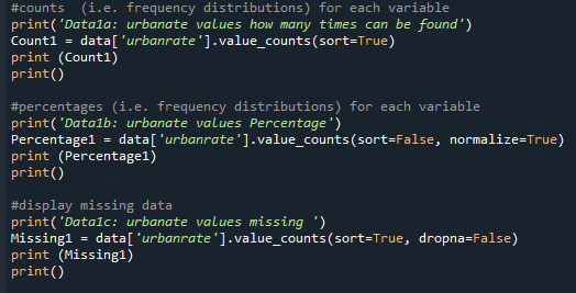
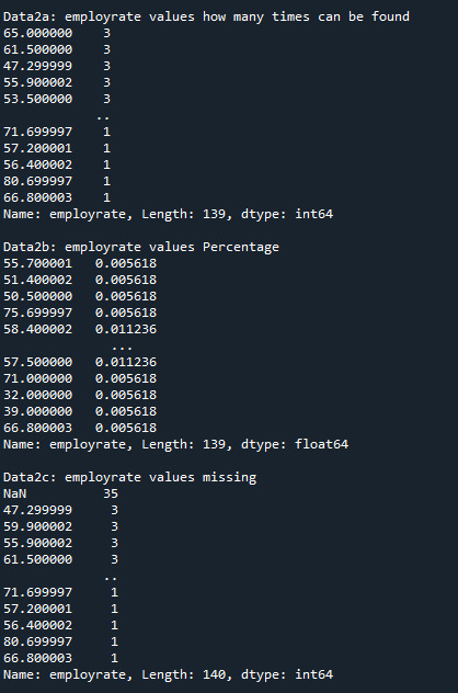
Print 'urbanrate' quantity, percentage and missing data:

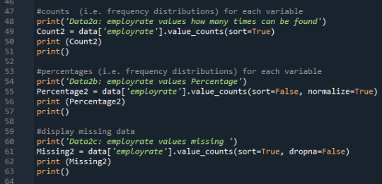
Print 'employrate' quantity, percentage and missing data:

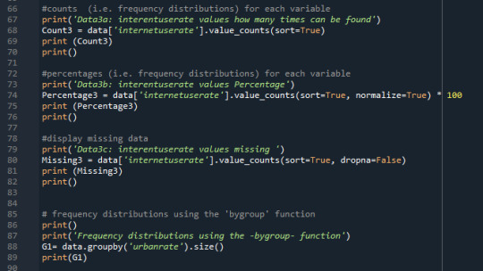
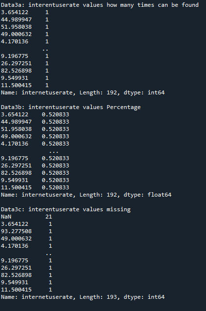
Print 'interentuserate' quantity, percentage and missing data:

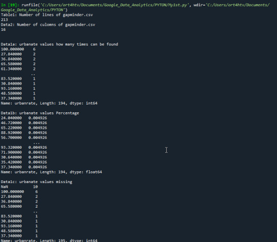
Output:

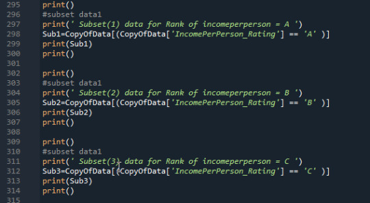
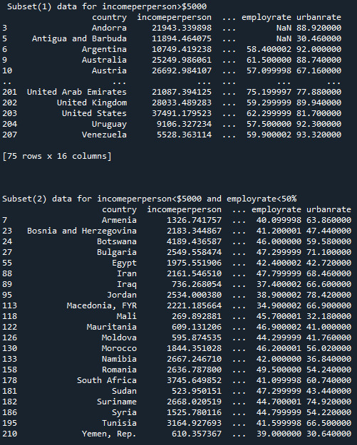
Creating subsets:

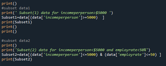
Output Subsets:

Copy of subset:

Summary:

Here I created frequency distributions displayed as count & percentage, also displays the missing data.

[igmpi]

Explore IGMPI’s Big Data Analytics program, designed for professionals seeking expertise in data-driven decision-making. Learn advanced analytics techniques, data mining, machine learning, and business intelligence tools to excel in the fast-evolving world of big data.

[infoveave]

Retailers face inventory mismanagement, demand fluctuations, and poor customer insights, impacting sales and profitability. Infoveave Pvt. Ltd. delivers retail analytics solutions, utilizing AI to track consumer behavior, forecast demand, and optimize pricing. With real-time data, retailers enhance supply chain efficiency, boost customer engagement, and maximize revenue through data-driven strategies.

[findyiot]

Human Factors: Decision making in the real world

It’s not enough for one person to know what happened yesterday—teams need to spot long-term trends to predict anomalies. Data is streaming, so static analysis doesn’t cut it. Unparsed data dumps don’t help. Being able to visualize data through dashboards or graphs helps to make sense of patterns. It is not about becoming data scientists. You do not need a degree in mechanics to drive a car. Your driving instructor tells you in simple terms how an engine works, where the oil goes, how to turn the steering wheel and which pedal to press.

Data should not be siloed. Maintenance, logistics, management, production teams — everyone needs to know some basics to make cohesive decisions. Cross-functional training is a key element to a deployment. There is a natural reluctance to embrace new things. Knowledge empowers and concurrently dispels fear of change. In hierarchical organizations there can be an aversion to the wider distribution of real-time information outside the management cadre. Inertia comes bottom up or top down, usually it is both at the same time.

[mitsdedistance]

SQL & Power BI Certification | MITSDE

Enhance your career with MITSDE’s Online Power BI Certification Course! This comprehensive program equips you with essential skills in data visualization, analytics, and business intelligence, helping you make data-driven decisions. Learn to create interactive dashboards, generate insightful reports, and analyze business trends effectively. Designed for professionals and beginners alike, this course offers hands-on training and expert guidance to boost your expertise. Stay ahead in the competitive job market—enroll today and transform your data analysis skills with Power BI!

[specbee-c-s]

Exploring the Drupal Views module

Sure you’ve worked with the Views module in Drupal but have you made the most of it? Get the full breakdown of its features and learn how to create dynamic displays in this article.

[newfangled-vady]

VADY – Transforming Raw Data into Strategic Masterpieces

VADY excels at transforming raw, unprocessed data into valuable business assets. Using AI, we refine complex data sets and convert them into actionable insights that drive strategic decision-making. Whether it's improving operational efficiency, enhancing customer experiences, or identifying new market opportunities, VADY ensures that data is a driving force behind your business’s growth. We offer businesses the tools to unlock their data’s potential, turning it into a strategic masterpiece. With VADY, companies gain a clearer understanding of their landscape, enabling them to make informed decisions that enhance performance, innovation, and profitability for the long run.