poudelbibek - Tumblr blog

poudelbibek · 2 years ago

Text

Data Analysis tools Assignment 4: Moderator

Study topic:

Employment rate Vs Suicide rate

Variables of interest:

Flow sequence for a python program

Steps:

Read the csv file.

Convert the datas of interest to numeric

Select only the readable data (exclude null or NaN)

Run Pearson correlation test on overall data.

Convert the moderator “income per person” into categorical variable into 3 categories and name the new variable as “incomegrp” a. 1 – LOW INCOME countries b. 2 – MIDDLE INCOME countries c. 3 – HIGH INCOME countries

Run Pearson correlation test for each level of moderator.

Python program

#Importing libraries

import numpy as np

import pandas

import statsmodels.formula.api as smf

import statsmodels.stats.multicomp as multi

import scipy.stats

import seaborn

import matplotlib.pyplot as plt

#Reading the data csv file

data = pandas.read_csv('gapminder.csv')

### Suiciderate is response variable whereas employment rate is explanatory variable

#setting variables of interest to numeric and creating datasets for response and explanatory variables

data['suicideper100th'] = pandas.to_numeric(data['suicideper100th'],errors = 'coerce')

data['incomeperperson'] = pandas.to_numeric(data['incomeperperson'],errors = 'coerce')

data['employrate'] = pandas.to_numeric(data['employrate'],errors = 'coerce')

#Subset for data of interest

di = data[['suicideper100th', 'incomeperperson','employrate']].dropna()

#Calculating Pearson correlation coefficient on overall data

print (scipy.stats.pearsonr(di['employrate'], di['suicideper100th']))

Output:

(0.01753468728377806, 0.8241876850138514)

#Categorizing income per person to 3 different levels to make incomeperperson as a categorical explanatory variable as well

def incomegrp (row):

if row['incomeperperson'] <= 800:

return 1

elif row['incomeperperson'] <= 9000 :

return 2

elif row['incomeperperson'] > 9000:

return 3

di['incomegrp'] = di.apply (lambda row: incomegrp (row),axis=1)

#Subgrouping data according to income group levels

sub1=di[(di['incomegrp']== 1)]

sub2=di[(di['incomegrp']== 2)]

sub3=di[(di['incomegrp']== 3)]

#Running Pearson correlation coefficient test on each sub group

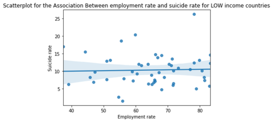
print ('Association between employment rate and suicide rate for LOW income countries')

print (scipy.stats.pearsonr(sub1['employrate'], sub1['suicideper100th']))

Output:

Association between employment rate and suicide rate for LOW income countries

(0.03469540098012962, 0.8109502633870055)

print ('Association between employment rate and suicide rate for MEDIUM income countries')

print (scipy.stats.pearsonr(sub2['employrate'], sub2['suicideper100th']))

Output:

Association between employment rate and suicide rate for MEDIUM income countries

(0.053355137933444076, 0.6539237810305579)

print ('Association between employment rate and suicide rate for HIGH income countries')

print (scipy.stats.pearsonr(sub1['employrate'], sub1['suicideper100th']))

Output:

Association between employment rate and suicide rate for HIGH income countries

(0.03469540098012962, 0.8109502633870055)

#Scatterplots

scat1 = seaborn.regplot(x="employrate", y="suicideper100th", data=sub1)

plt.xlabel('Employment rate')

plt.ylabel('Suicide rate')

plt.title('Scatterplot for the Association Between employment rate and suicide rate for LOW income countries')

print (scat1)

scat2 = seaborn.regplot(x="employrate", y="suicideper100th", data=sub2)

plt.xlabel('Employment rate')

plt.ylabel('Suicide rate')

plt.title('Scatterplot for the Association Between employment rate and suicide rate for LOW income countries')

print (scat2)

scat3 = seaborn.regplot(x="employrate", y="suicideper100th", data=sub3)

plt.xlabel('Employment rate')

plt.ylabel('Suicide rate')

plt.title('Scatterplot for the Association Between employment rate and suicide rate for LOW income countries')

print (scat3)

Discussion from Moderator tests:

When examining the association between employment rate with suicide rate, Pearson correlation test showed that suicide rate does not depend on employment rate (r = 0.01175 (very low) and p=0.824 > 0.05 significance level).

It was hypothesized that the income level of a country could be a moderator in this study. Hence, with countries sub-grouped into 3 different levels: low-income, middle-income, and high-income groups, Pearson correlation test to test an association of employment rate and suicide rate was conducted again on each group. Groupwise test again showed that for each group, the association was statistically insignificant:

Low-income countries - r = 0.0346 (very low) and p=0.65 > 0.05 significance level)

Middle-income countries - r = 0.0533 (very low) and p=0.65 > 0.05 significance level)

High-income countries - r = -0.133 (very low) and p=0.41 > 0.05 significance level)

One thing to notice from the results and the scatter plot was: As the employment rate increased, suicide rate increased as well for low and middle-income countries whereas it decreased for high-income countries (even though the slope was extremely small).

0 notes

poudelbibek · 2 years ago

Text

Data Analysis tools Assignment 3: Correlation coefficient

Reminder (research problem and defined variables)

Study topic:

Primary topic

Suicide rate Vs. incomeperperson

Variables of interest:

suicideper100th: This data gives the number of suicide due to self-inflicted injury per 100,000 people in any particular country. This rate is calculated as if all countries had the same age composition of the population. The data is based on the “Global burden of disease study” from WHO.

incomeperperson: The data contains GDP per capita in US dollars divided by midyear population. This data is calculated adjusting the global inflation (without making deductions for the depreciation of fabricated assets or for depletion and degradation of natural resources). The data was provided by world bank.

Flow sequence for a python program

Steps:

Read the csv file

Convert data of interest to numeric

Select only readable data (exclude null or NaN)

Generate scatter plot of response variable (suicideper100th) vs. explanatory variable (incomeperperson)

Generate the Pearson-correlation coefficient.

Python program

#Importing libraries

import numpy

import pandas

import statsmodels.formula.api as smf

import statsmodels.stats.multicomp as multi

import scipy.stats

import seaborn

import matplotlib.pyplot as plt

#Reading the data csv file

data = pandas.read_csv('gapminder.csv')

### Suiciderate is response variable whereas incomeperperson is explanatory variable

#setting variables of interest to numeric and creating datasets for response and explanatory variables

data['suicideper100th'] = pandas.to_numeric(data['suicideper100th'],errors = 'coerce')

data['incomeperperson'] = pandas.to_numeric(data['incomeperperson'],errors = 'coerce')

#Subset for data of interest

dataofinterest = data[['suicideper100th', 'incomeperperson']].dropna()

dataofinterest

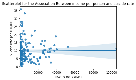
#Scatter plot

scat1 = seaborn.regplot(x="incomeperperson", y="suicideper100th", fit_reg=True, data=dataofinterest)

plt.xlabel('Income per person')

plt.ylabel('Suicide rate per 100,000')

plt.title('Scatterplot for the Association Between income per person and suicide rate')

#Pearson correlation coefficient

data_clean=dataofinterest.dropna()

print ('Association Between income per person and suicide rate')

print (scipy.stats.pearsonr(data_clean['incomeperperson'], data_clean['suicideper100th']))

Output:

Association Between income per person and suicide rate

(0.0065552893496113665, 0.9302086466053822)

Discussion from Correlation coefficient test:

When examining the association between income per person with suicide rate, correlation coefficient (r) was found to 0.00655, which is positive – so it shows a higher suicide rate with higher income); but the value is extremely small (nearly zero). This means the correlation between income per person to suicide rate is basically none. Also, the p-value is (p=0.93 > 0.05), which also indicates statistically insignificant relationship.

This can be seen from scatter plot as well. The graph looks like a straight horizontal line [nearly a y=0 line]. This again points to extremely low (close to none) association between income per person and suicide rate.

0 notes

poudelbibek · 2 years ago

Text

Data Analysis tools Assignment 2 : Chi-square tests

Reminder (research problem and defined variables)

Study topic:

Primary topic

Suicide rate Vs. Polityscore

Variables of interest:

Flow sequence for a python program

Steps:

Read the csv file.

Convert the datas of interest to numeric

Select only the readable data (exclude null or NaN)

Convert the suicideper100th into categorical variable into 2 categories and name the new variable as “suicide_severity” 0 – not severe 1 – severe

Convert the polityscore categorical variable into only 4 categories and name new variable as “broadpolityscore. -10 to -6: 0- Very poor -5 to 0: 1- Poor 1 to 5: 2- Okay 6 to 10: 3- Good

Run Chi-square test.

Run post- hoc test.

Python program

#Importing libraries

import numpy

import pandas

import statsmodels.formula.api as smf

import statsmodels.stats.multicomp as multi

# bug fix for display formats to avoid run time errors

pandas.set_option('display.float_format', lambda x:'%.2f'%x)

#Reading the data csv file

data = pandas.read_csv('gapminder.csv')

### Suiciderate is response variable whereas polityscore is explanatory variable

#setting variables of interest to numeric and creating datasets for response and explanatory variables

data['suicideper100th'] = pandas.to_numeric(data['suicideper100th'],errors = 'coerce')

data['polityscore'] = pandas.to_numeric(data['polityscore'],errors = 'coerce')

#Subset for data of interest

dataofinterest = data[['suicideper100th', 'polityscore']].dropna()

dataofinterest

#Categorizing political score data into 4 categories and giving it a name of “broadpolityscore”

#-10 to -5: Very poor à 0

# -5 to 0: Poor à 1

# 0 to 5: Okay à 2

#6 to 10: Good à 3

di = dataofinterest

#di["bins"] = pandas.cut(di["suicideper100th"], bins = 2)

bins = [-10,-5,0,5,10]

group_names = ['Very poor', 'Poor', 'Okay', 'Good']

categories = pandas.cut(dataofinterest['polityscore'], bins)

categories.value_counts(sort=False, dropna=False)

#Creating new data set for bincenters

di['bins']= pandas.cut(dataofinterest['polityscore'], bins)

di["bin_centers"] = di["bins"].apply(lambda x: x.mid)

di['bin_centers'] = pandas.to_numeric(di['bin_centers'],errors = 'coerce')

#Assigning broadpolityscore according to bin_center value

tot = len(di['bins'])

print(tot)

di.reset_index(drop=True, inplace=True)

di = di.assign(broadpolityscore=" ")

for j in range(tot):

#print(di['bin_centers'][j])

if di['bin_centers'][j]<-5:

score = 0

di['broadpolityscore'][j] = score

elif -5<di['bin_centers'][j]<0:

score = 1

di['broadpolityscore'][j] = score

elif 0<di['bin_centers'][j]<5:

score = 2

di['broadpolityscore'][j] = score

else:

score = 3

di['broadpolityscore'][j] = score

#Creating categorical response variable “suicide_severity”

#di["bins"] = pandas.cut(di["suicideper100th"], bins = 2)

di['bins'] = pandas.qcut(di['suicideper100th'], q=2)

di["bin_centers"] = di["bins"].apply(lambda x: x.mid)

#Assign suicide severity score

di.reset_index(drop=True, inplace=True)

print(len(di['bin_centers']))

di = di.assign(suicide_severity=" ")

for j in range(len(di['suicide_severity'])):

#print(di['bin_centers'][j])

if di['bin_centers'][j]<5:

bin_centers_cat = 0

di['suicide_severity'][j] = bin_centers_cat

else:

bin_centers_cat = 1

di['suicide_severity'][j] = bin_centers_cat

Results

# contingency table of observed counts

ct1=pandas.crosstab(di['suicide_severity'], di['broadpolityscore'])

print (ct1)

broadpolityscore 0 1 2 3

suicide_severity

0 13 15 8 44

1 10 12 11 46

# column percentages

colsum=ct1.sum(axis=0)

colpct=ct1/colsum

print(colpct)

broadpolityscore 0 1 2 3

suicide_severity

0 0.565217 0.555556 0.421053 0.488889

1 0.434783 0.444444 0.578947 0.511111

# chi-square

print ('chi-square value, p value, expected counts')

cs1= scipy.stats.chi2_contingency(ct1)

print (cs1)

chi-square value, p value, expected counts

(1.2365259392289194, 0.744257866100584, 3, array([[11.57232704, 11.42767296],

[13.58490566, 13.41509434],

[ 9.55974843, 9.44025157],

[45.28301887, 44.71698113]]))

# graph percent with suicide severity Vs broad political score

seaborn.factorplot(x="broadpolityscore", y="suicide_severity", data=di, kind="bar", ci=None)

plt.xlabel('Broad political score')

plt.ylabel('Suicide severity')

#Post-hoc Chi square

recode2 = {0:0, 1:1}

di['comp0v1']= di['broadpolityscore'].map(recode2)

# contingency table of observed counts

ct2=pandas.crosstab(di['suicide_severity'], di['comp0v1'])

print (ct2)

# column percentages

colsum=ct2.sum(axis=0)

colpct=ct2/colsum

print(colpct)

print ('chi-square value, p value, expected counts')

cs2= scipy.stats.chi2_contingency(ct2)

print (cs2)

Output:

comp0v1 0.0 1.0

suicide_severity

0 13 15

1 10 12

comp0v1 0.0 1.0

suicide_severity

0 0.565217 0.555556

1 0.434783 0.444444

chi-square value, p value, expected counts

(0.04718510153292781, 0.8280358709711078, 1, array([[12.88, 15.12],

[10.12, 11.88]]))

recode3 = {0:0, 2:2}

di['comp0v2']= di['broadpolityscore'].map(recode3)

# contingency table of observed counts

ct3=pandas.crosstab(di['suicide_severity'], di['comp0v2'])

print (ct3)

# column percentages

colsum=ct3.sum(axis=0)

colpct=ct3/colsum

print(colpct)

print ('chi-square value, p value, expected counts')

cs3= scipy.stats.chi2_contingency(ct3)

print (cs3)

Output:

comp0v2 0.0 2.0

suicide_severity

0 13 8

1 10 11

comp0v2 0.0 2.0

suicide_severity

0 0.565217 0.421053

1 0.434783 0.578947

chi-square value, p value, expected counts

(0.38443935926773454, 0.5352368901951887, 1, array([[11.5, 9.5],

[11.5, 9.5]]))

recode4 = {0:0, 3:3}

di['comp0v3']= di['broadpolityscore'].map(recode4)

# contingency table of observed counts

ct4=pandas.crosstab(di['suicide_severity'], di['comp0v3'])

print (ct4)

# column percentages

colsum=ct4.sum(axis=0)

colpct=ct4/colsum

print(colpct)

print ('chi-square value, p value, expected counts')

cs4= scipy.stats.chi2_contingency(ct4)

print (cs4)

Output:

comp0v3 0.0 3.0

suicide_severity

0 13 44

1 10 46

comp0v3 0.0 3.0

suicide_severity

0 0.565217 0.488889

1 0.434783 0.511111

chi-square value, p value, expected counts

(0.17618839520298316, 0.6746695456425893, 1, array([[11.60176991, 45.39823009],

[11.39823009, 44.60176991]]))

recode5 = {1:1, 2:2}

di['comp1v2']= di['broadpolityscore'].map(recode5)

# contingency table of observed counts

ct5=pandas.crosstab(di['suicide_severity'], di['comp1v2'])

print (ct5)

# column percentages

colsum=ct5.sum(axis=0)

colpct=ct5/colsum

print(colpct)

print ('chi-square value, p value, expected counts')

cs5= scipy.stats.chi2_contingency(ct5)

print (cs5)

Output:

comp1v2 1.0 2.0

suicide_severity

0 15 8

1 12 11

comp1v2 1.0 2.0

suicide_severity

0 0.555556 0.421053

1 0.444444 0.578947

chi-square value, p value, expected counts

(0.3586744639376218, 0.5492433274240123, 1, array([[13.5, 9.5],

[13.5, 9.5]]))

recode6 = {1:1, 3:3}

di['comp1v3']= di['broadpolityscore'].map(recode6)

# contingency table of observed counts

ct6=pandas.crosstab(di['suicide_severity'], di['comp1v3'])

print (ct6)

# column percentages

colsum=ct6.sum(axis=0)

colpct=ct6/colsum

print(colpct)

print ('chi-square value, p value, expected counts')

cs6= scipy.stats.chi2_contingency(ct6)

print (cs6)

Output:

comp1v3 1.0 3.0

suicide_severity

0 15 44

1 12 46

comp1v3 1.0 3.0

suicide_severity

0 0.555556 0.488889

1 0.444444 0.511111

chi-square value, p value, expected counts

(0.15072326125073082, 0.697845139978909, 1, array([[13.61538462, 45.38461538],

[13.38461538, 44.61538462]]))

recode7 = {2:2, 3:3}

di['comp2v3']= di['broadpolityscore'].map(recode7)

# contingency table of observed counts

ct7=pandas.crosstab(di['suicide_severity'], di['comp2v3'])

print (ct7)

# column percentages

colsum=ct7.sum(axis=0)

colpct=ct7/colsum

print(colpct)

print ('chi-square value, p value, expected counts')

cs7= scipy.stats.chi2_contingency(ct7)

print (cs7)

Output:

comp2v3 2.0 3.0

suicide_severity

0 8 44

1 11 46

comp2v3 2.0 3.0

suicide_severity

0 0.421053 0.488889

1 0.578947 0.511111

chi-square value, p value, expected counts

(0.08133967256197186, 0.7754900707886289, 1, array([[ 9.06422018, 42.93577982],

[ 9.93577982, 47.06422018]]))

Discussion from Chi-square test models:

When examining the association between political score with suicide rate, Chi-square showed that suicide rate does not depend on political score (p=0.744 > significance level). The degree of freedom was 3 (explanatory variable (4) – 1). Looking at the bar chart of suicide severity vs broad political score, the means (suicide_severity) of each political score level [polityscore, 0 – 43.4%; polityscore, 1 – 44.4% polityscore, 2 – 57.9% ; polityscore, 3 – 51.1% ] look really close with each other further confirming not much of an association between political score and the suicide severity.

Post hoc Chi-square revealed the same finding as Chi-square -> that the dependence of political score [divided into 4 categories as a categorical explanatory variable] and suicide severity [categorical response variable] were not statistically significant in each case (p value in each case was higher than the significance level). Hence accepting the null hypothesis will be reasonable here. All the comparisons were statistically similar.

0 notes

poudelbibek · 2 years ago

Text

Data Analysis tools Assignment 1 [ Suicide rate Vs political score]

Study topic:

Primary topic

Suicide rate Vs. Polityscore

Variables of interest:

Polityscore: This is an interesting data where there is a score ranging from -10 to 10. The score indicates how politically free the country is with -10 being the country with least democratic and free nature and 10 being the highest.

Flow sequence for a python program

Steps:

Python program

#Importing libraries

import numpy

import pandas

import statsmodels.formula.api as smf

import statsmodels.stats.multicomp as multi

# bug fix for display formats to avoid run time errors

pandas.set_option('display.float_format', lambda x:'%.2f'%x)

#Reading the data csv file

data = pandas.read_csv('gapminder.csv')

### Suiciderate is response variable whereas polityscore is explanatory variable

#setting variables of interest to numeric and creating datasets for response and explanatory variables

data['suicideper100th'] = pandas.to_numeric(data['suicideper100th'],errors = 'coerce')

data['polityscore'] = pandas.to_numeric(data['polityscore'],errors = 'coerce')

#Subset for data of interest

dataofinterest = data[['suicideper100th', 'polityscore']].dropna()

dataofinterest

#Categorizing political score data into 4 categories and giving it a name of “broadpolityscore”

#-10 to -5: Very poor à 0

# -5 to 0: Poor à 1

# 0 to 5: Okay à 2

#6 to 10: Good à 3

di = dataofinterest

#di["bins"] = pandas.cut(di["suicideper100th"], bins = 2)

bins = [-10,-5,0,5,10]

group_names = ['Very poor', 'Poor', 'Okay', 'Good']

categories = pandas.cut(dataofinterest['polityscore'], bins)

categories.value_counts(sort=False, dropna=False)

#Creating new data set for bincenters

di['bins']= pandas.cut(dataofinterest['polityscore'], bins)

di["bin_centers"] = di["bins"].apply(lambda x: x.mid)

di['bin_centers'] = pandas.to_numeric(di['bin_centers'],errors = 'coerce')

#Assigning broadpolityscore according to bin_center value

tot = len(di['bins'])

print(tot)

di.reset_index(drop=True, inplace=True)

di = di.assign(broadpolityscore=" ")

for j in range(tot):

#print(di['bin_centers'][j])

if di['bin_centers'][j]<-5:

score = 0

di['broadpolityscore'][j] = score

elif -5<di['bin_centers'][j]<0:

score = 1

di['broadpolityscore'][j] = score

elif 0<di['bin_centers'][j]<5:

score = 2

di['broadpolityscore'][j] = score

else:

score = 3

di['broadpolityscore'][j] = score

#Mean

print ('means for numcigmo_est by major depression status')

m1= di.groupby('broadpolityscore').mean()

print (m1)

Output: Mean:

suicideper100th

broadpolityscore

0 9.304686

1 9.262136

2 10.299483

3 10.397801

Output: Standard deviation:

suicideper100th

broadpolityscore

0 7.949021

1 6.242215

2 5.868889

3 6.351548

#OLS model - ANOVA

model1 = smf.ols(formula='suicideper100th ~ C(broadpolityscore)', data=di)

results1 = model1.fit()

print (results1.summary())

Output:

OLS Regression Results

==============================================================================

Dep. Variable: suicideper100th R-squared: 0.006

Model: OLS Adj. R-squared: -0.013

Method: Least Squares F-statistic: 0.3248

Date: Mon, 03 Apr 2023 Prob (F-statistic): 0.807

Time: 16:54:34 Log-Likelihood: -521.99

No. Observations: 159 AIC: 1052.

Df Residuals: 155 BIC: 1064.

Df Model: 3

Covariance Type: nonrobust

============================================================================================

coef std err t P>|t| [0.025 0.975]

--------------------------------------------------------------------------------------------

Intercept 9.3047 1.362 6.831 0.000 6.614 11.995

C(broadpolityscore)[T.1] -0.0425 1.854 -0.023 0.982 -3.704 3.619

C(broadpolityscore)[T.2] 0.9948 2.025 0.491 0.624 -3.005 4.995

C(broadpolityscore)[T.3] 1.0931 1.526 0.716 0.475 -1.922 4.108

==============================================================================

Omnibus: 47.317 Durbin-Watson: 2.134

Prob(Omnibus): 0.000 Jarque-Bera (JB): 91.187

Skew: 1.384 Prob(JB): 1.58e-20

Kurtosis: 5.471 Cond. No. 6.73

==============================================================================

Warnings:

[1] Standard Errors assume that the covariance matrix of the errors is correctly specified.

#Post-hoc ANOVA

mc1 = multi.MultiComparison(di['suicideper100th'], di['broadpolityscore'])

res1 = mc1.tukeyhsd()

print(res1.summary())

Output:

Multiple Comparison of Means - Tukey HSD, FWER=0.05

===================================================

group1 group2 meandiff p-adj lower upper reject

---------------------------------------------------

0 1 -0.0425 0.9 -4.8566 4.7715 False

0 2 0.9948 0.9 -4.2649 6.2545 False

0 3 1.0931 0.8833 -2.8708 5.0571 False

1 2 1.0373 0.9 -4.043 6.1177 False

1 3 1.1357 0.8408 -2.5871 4.8584 False

2 3 0.0983 0.9 -4.1851 4.3817 False

---------------------------------------------------

Discussion from ANOVA models:

When examining the association between political score with suicide rate, ANOVA showed that suicide rate does not depend on political score (p>0.05). Looking at the mean suicide rate values of different political score categories, all the means were very close to each other [9.30,9.26,10.29 and 10.39].

Post hoc ANOVA revealed that the dependence of political score [divided into 4 categories as a categorical explanatory variable] and suicide rate [ quantitative response variable] were not statistically significant p= 0.807 (which is p>0.05) andF[3,159] = 0.3248. Post hoc comparison between categories of political score also revealed that none of the political scores associated significantly [all had p>0.05, hence accepting the null hypothesis] with suicide rate. All the comparisons were statistically similar.

0 notes

poudelbibek · 2 years ago

Text

Regression modeling in practice Assignment 4

Regression modeling Assignment 4

Reminder (research problem and defined variables)

Study topic:

Primary topic

Suicide rate Vs. Income per person

Variables of interest:

Secondary topic

Suicide rate Vs. Employrate and polityscore

Flow sequence for a python program

Steps:

Read the csv file.

Convert the datas of interest to numeric

Select only the readable data (exclude null or NaN)

Bin the suicide rate data and assign them into 2 binary categories a. [New variable creation: Suicide severity] b.Suicide severity = 0 if suicideper100th is less than 5: =1 if more than or equal to 5

Logistic regression on suicide severity vs incomedata

Logistic regression on suicide severity vs incomedata categorized into different levels (0.0, 7994.471] 116 - Income level 1 (7994.471, 15988.941] 14 – Income level 2 (15988.941, 23983.412] 5 – Income level 3 (23983.412, 31977.882] 10 – Income level 4 (31977.882, 39972.353] 7 – Income level 5

Logistic regression on suicide severity vs employdata and politydata and the various combinations

Print the OR data and confidence intervals.

Python program

#Importing libraries

import numpy as np

import pandas as pandas

import statsmodels.api as sm

import statsmodels.formula.api as smf

import seaborn

import matplotlib.pyplot as plt

# bug fix for display formats to avoid run time errors

pandas.set_option('display.float_format', lambda x:'%.2f'%x)

#Reading the data csv file

data = pandas.read_csv('gapminder.csv')

### Suiciderate is response whereas incomeperperson is explanatory variable

#setting variables of interest to numeric and creating datasets for response and explanatory variables

data['suicideper100th'] = pandas.to_numeric(data['suicideper100th'],errors = 'coerce')

data['incomeperperson'] = pandas.to_numeric(data['incomeperperson'],errors = 'coerce')

data['employrate'] = pandas.to_numeric(data['employrate'],errors = 'coerce')

data['polityscore'] = pandas.to_numeric(data['polityscore'],errors = 'coerce')

#Subset for data of interest

dataofinterest = data[['country','incomeperperson','suicideper100th' ,'employrate','polityscore']]

#Filtering countries with valid data of interests (exlude null columns)

unnulldataonly = dataofinterest[dataofinterest['suicideper100th'].notna() & dataofinterest['incomeperperson'].notna() & dataofinterest['employrate'].notna() & dataofinterest['polityscore'].notna()]

incomeonly = unnulldataonly.incomeperperson

suicideonly = unnulldataonly.suicideper100th

polityonly = unnulldataonly.polityscore

employrateonly = unnulldataonly.employrate

unnullcountry = unnulldataonly.country#Center the explanatory variable i.e. incomeperperson

#Integrating data of interests with centered explanatory variable

di = pandas.DataFrame(unnullcountry)

#Merge centered income data and suicide data into new dataframe

di = pandas.concat([di,suicideonly,incomeonly,employrateonly,polityonly],axis=1)

#di["bins"] = pandas.cut(di["suicideper100th"], bins = 2)

di['bins'] = pandas.qcut(di['suicideper100th'], q=2)

di["bin_centers"] = di["bins"].apply(lambda x: x.mid)

#Assign suicide severity score (creating binary categorical response variable)

di.reset_index(drop=True, inplace=True)

print(len(di['bin_centers']))

di = di.assign(suicide_severity=" ")

for j in range(len(di['suicide_severity'])):

#print(di['bin_centers'][j])

if di['bin_centers'][j]<5:

bin_centers_cat = 0

di['suicide_severity'][j] = bin_centers_cat

else:

bin_centers_cat = 1

di['suicide_severity'][j] = bin_centers_cat

#setting variables of interest to numeric and creating datasets for response and explanatory variables

di['suicideper100th'] = pandas.to_numeric(di['suicideper100th'],errors = 'coerce')

di['incomeperperson'] = pandas.to_numeric(di['incomeperperson'],errors = 'coerce')

di['suicide_severity'] = pandas.to_numeric(di['suicide_severity'],errors = 'coerce')

di['employrate'] = pandas.to_numeric(di['employrate'],errors = 'coerce')

di['polityscore'] = pandas.to_numeric(di['polityscore'],errors = 'coerce')

#Logistic regression on suicide severity vs income per person

lreg1 = smf.logit(formula = 'suicide_severity ~ incomeperperson', data = di).fit()

print (lreg1.summary())

# odds ratios

print ("Odds Ratios")

print (numpy.exp(lreg1.params))

Output

Logit Regression Results

==============================================================================

Dep. Variable: suicide_severity No. Observations: 152

Model: Logit Df Residuals: 150

Method: MLE Df Model: 1

Date: Fri, 03 Mar 2023 Pseudo R-squ.: 0.007466

Time: 11:15:08 Log-Likelihood: -104.57

converged: True LL-Null: -105.36

Covariance Type: nonrobust LLR p-value: 0.2097

===================================================================================

coef std err z P>|z| [0.025 0.975]

-----------------------------------------------------------------------------------

Intercept -0.1400 0.197 -0.710 0.478 -0.527 0.247

incomeperperson 2.108e-05 1.7e-05 1.237 0.216 -1.23e-05 5.45e-05

===================================================================================

Odds Ratios

Intercept 0.87

incomeperperson 1.00

dtype: float64

# odd ratios with 95% confidence intervals

params = lreg1.params

conf = lreg1.conf_int()

conf['OR'] = params

conf.columns = ['Lower CI', 'Upper CI', 'OR']

print (numpy.exp(conf))

Output:

Lower CI Upper CI OR

Intercept 0.59 1.28 0.87

incomeperperson 1.00 1.00 1.00

# logistic regression with incomeperperson and employrate

lreg2 = smf.logit(formula = 'suicide_severity ~ incomeperperson + employrate', data = di).fit()

print (lreg2.summary())

# odd ratios with 95% confidence intervals

params = lreg2.params

conf = lreg2.conf_int()

conf['OR'] = params

conf.columns = ['Lower CI', 'Upper CI', 'OR']

print (numpy.exp(conf))

Output:

Logit Regression Results

==============================================================================

Dep. Variable: suicide_severity No. Observations: 152

Model: Logit Df Residuals: 149

Method: MLE Df Model: 2

Date: Fri, 03 Mar 2023 Pseudo R-squ.: 0.01781

Time: 11:15:14 Log-Likelihood: -103.48

converged: True LL-Null: -105.36

Covariance Type: nonrobust LLR p-value: 0.1531

===================================================================================

coef std err z P>|z| [0.025 0.975]

-----------------------------------------------------------------------------------

Intercept -1.5408 0.980 -1.573 0.116 -3.461 0.379

incomeperperson 2.245e-05 1.73e-05 1.297 0.195 -1.15e-05 5.64e-05

employrate 0.0235 0.016 1.462 0.144 -0.008 0.055

===================================================================================

Lower CI Upper CI OR

Intercept 0.03 1.46 0.21

incomeperperson 1.00 1.00 1.00

employrate 0.99 1.06 1.02

# logistic regression with polityscore

lreg3 = smf.logit(formula = 'suicide_severity ~ polityscore', data = di).fit()

print (lreg3.summary())

# odd ratios with 95% confidence intervals

print ("Odds Ratios")

params = lreg3.params

conf = lreg3.conf_int()

conf['OR'] = params

conf.columns = ['Lower CI', 'Upper CI', 'OR']

print (numpy.exp(conf))

Output

Logit Regression Results

==============================================================================

Dep. Variable: suicide_severity No. Observations: 152

Model: Logit Df Residuals: 150

Method: MLE Df Model: 1

Date: Fri, 03 Mar 2023 Pseudo R-squ.: 0.008922

Time: 11:15:19 Log-Likelihood: -104.42

converged: True LL-Null: -105.36

Covariance Type: nonrobust LLR p-value: 0.1703

===============================================================================

coef std err z P>|z| [0.025 0.975]

-------------------------------------------------------------------------------

Intercept -0.1396 0.193 -0.722 0.470 -0.518 0.239

polityscore 0.0360 0.026 1.362 0.173 -0.016 0.088

===============================================================================

Odds Ratios

Lower CI Upper CI OR

Intercept 0.60 1.27 0.87

polityscore 0.98 1.09 1.04

# logistic regression with incomeperperson and polityscore

lreg4 = smf.logit(formula = 'suicide_severity ~ incomeperperson + polityscore', data = di).fit()

print (lreg2.summary())

# odd ratios with 95% confidence intervals

params = lreg4.params

conf = lreg4.conf_int()

conf['OR'] = params

conf.columns = ['Lower CI', 'Upper CI', 'OR']

print (numpy.exp(conf))

Output

Logit Regression Results

==============================================================================

Dep. Variable: suicide_severity No. Observations: 152

Model: Logit Df Residuals: 149

Method: MLE Df Model: 2

Date: Fri, 03 Mar 2023 Pseudo R-squ.: 0.01278

Time: 13:54:07 Log-Likelihood: -104.01

converged: True LL-Null: -105.36

Covariance Type: nonrobust LLR p-value: 0.2602

===================================================================================

coef std err z P>|z| [0.025 0.975]

-----------------------------------------------------------------------------------

Intercept -0.2174 0.212 -1.027 0.304 -0.632 0.197

incomeperperson 1.586e-05 1.77e-05 0.894 0.371 -1.89e-05 5.06e-05

polityscore 0.0290 0.027 1.055 0.292 -0.025 0.083

===================================================================================

Lower CI Upper CI OR

Intercept 0.53 1.22 0.80

incomeperperson 1.00 1.00 1.00

polityscore 0.98 1.09 1.03

#Categorizing income per person to 5 different levels to make incomeperperson as a categorical explanatory variable as well

incomeperperson_bins = pandas.cut(di['incomeperperson'], bins = np.linspace(0,di['incomeperperson'].max(),num=6))

Output

(0.0, 7994.471] 116

(7994.471, 15988.941] 14

(15988.941, 23983.412] 5

(23983.412, 31977.882] 10

(31977.882, 39972.353] 7

#Taking mean of bins and reading value counts

di['incomeperperson_bins'] = pandas.cut(di['incomeperperson'], bins = np.linspace(0,di['incomeperperson'].max(),num=6))

di["income_bin_centers"] = di["incomeperperson_bins"].apply(lambda x: x.mid)

di["income_bin_centers"]=di["income_bin_centers"].apply(lambda x:round(x,2))

print(di["income_bin_centers"].value_counts())

Output

3997.24 116

11991.71 14

27980.65 10

35975.12 7

19986.18 5

#Assigning income level

di = di.assign(incomelevel=" ")

di.loc[di['income_bin_centers']==3997.24, 'incomelevel'] = '1'

di.loc[di['income_bin_centers']==11991.71 , 'incomelevel'] = '2'

di.loc[di['income_bin_centers']==27980.65, 'incomelevel'] = '3'

di.loc[di['income_bin_centers']==35975.12, 'incomelevel'] = '4'

di.loc[di['income_bin_centers']==19986.18 , 'incomelevel'] = '5'

di['incomelevel'] = pandas.to_numeric(di['incomelevel'],errors = 'coerce')

di['income_bin_centers'] = pandas.to_numeric(di['income_bin_centers'],errors = 'coerce')

# logistic regression with incomelevel and employrate

lreg6 = smf.logit(formula = 'suicide_severity ~ incomelevel', data = di).fit()

print (lreg6.summary())

# odd ratios with 95% confidence intervals

params = lreg6.params

conf = lreg6.conf_int()

conf['OR'] = params

conf.columns = ['Lower CI', 'Upper CI', 'OR']

print (numpy.exp(conf))

Output

Logit Regression Results

==============================================================================

Dep. Variable: suicide_severity No. Observations: 152

Model: Logit Df Residuals: 150

Method: MLE Df Model: 1

Date: Fri, 03 Mar 2023 Pseudo R-squ.: 0.005051

Time: 11:52:28 Log-Likelihood: -104.83

converged: True LL-Null: -105.36

Covariance Type: nonrobust LLR p-value: 0.3022

===============================================================================

coef std err z P>|z| [0.025 0.975]

-------------------------------------------------------------------------------

Intercept -0.2456 0.289 -0.849 0.396 -0.813 0.321

incomelevel 0.1650 0.162 1.020 0.308 -0.152 0.482

===============================================================================

Lower CI Upper CI OR

Intercept 0.44 1.38 0.78

incomelevel 0.86 1.62 1.18

# logistic regression with incomelevel of incomelevel 2 and employrate

lreg6 = smf.logit(formula = 'suicide_severity ~ C(incomelevel,Treatment(reference=2))', data = di).fit()

print (lreg6.summary())

# odd ratios with 95% confidence intervals

params = lreg6.params

conf = lreg6.conf_int()

conf['OR'] = params

conf.columns = ['Lower CI', 'Upper CI', 'OR']

print (numpy.exp(conf))

Output:

Logit Regression Results

==============================================================================

Dep. Variable: suicide_severity No. Observations: 152

Model: Logit Df Residuals: 147

Method: MLE Df Model: 4

Date: Fri, 03 Mar 2023 Pseudo R-squ.: 0.02369

Time: 11:53:31 Log-Likelihood: -102.86

converged: True LL-Null: -105.36

Covariance Type: nonrobust LLR p-value: 0.2882

===============================================================================================================

coef std err z P>|z| [0.025 0.975]

---------------------------------------------------------------------------------------------------------------

Intercept -0.0690 0.186 -0.371 0.710 -0.433 0.295

C(incomelevel, Treatment(reference=1))[T.2] -0.2187 0.571 -0.383 0.702 -1.338 0.901

C(incomelevel, Treatment(reference=1))[T.3] 0.4745 0.672 0.706 0.480 -0.842 1.791

C(incomelevel, Treatment(reference=1))[T.4] 1.8608 1.096 1.698 0.090 -0.287 4.009

C(incomelevel, Treatment(reference=1))[T.5] -0.3365 0.932 -0.361 0.718 -2.162 1.489

===============================================================================================================

Lower CI Upper CI OR

Intercept 0.65 1.34 0.93

C(incomelevel, Treatment(reference=1))[T.2] 0.26 2.46 0.80

C(incomelevel, Treatment(reference=1))[T.3] 0.43 6.00 1.61

C(incomelevel, Treatment(reference=1))[T.4] 0.75 55.08 6.43

C(incomelevel, Treatment(reference=1))[T.5] 0.12 4.43 0.71

Conclusions:

Income per person was not associated with suicide severity (OR=1, 95% CI = 1.0-1.0, p = 0.216).

Not major association of polityscore with suicide severity was also observed (OR=1.04, 95% CI = 0.98-1.09, p = 0.173). Slightly higher tendency of suicide severity was seen in the countries with higher political score.

The logistic regression while accounting for both income per person and polity score showed following results. It clearly shows even with adjustment of polity score, income per person is statistically non-significant. There was not much hint of confounding.

Lower CI Upper CI OR p

Intercept 0.53 1.22 0.80 0.304

incomeperperson 1.00 1.00 1.00 0.371

polityscore 0.98 1.09 1.03 0.292

After binning income level into 5 different categories and saving them as income levels (1-5), logistic regression was carried out with incomelevel with suicide severity which showed following results. As the income level increases the probability of suicide severity also increases. Countries with higher income are seen to have experienced higher suicide severities. This was quite an interesting find because it contradicts a popular belief that the higher income countries are more content and have less suicidal severities.

Lower CI Upper CI OR p

Intercept 0.44 1.38 0.78 0.396

incomelevel 0.86 1.62 1.18 0.308

Also, logistic regression on suicide severity with incomelevel 2 as a treatment group was done. This result was interesting. It showed that even though there was still no statistically significant association between income level 2 to other income levels, one thing that was striking was that income level 4 had times more probability of having suicide severity than income level 2. Similarly, countries with income level 1 and 3 had 1.24 and 2 times more likely suicide severity. The countries with lowest suicide severity were with income level 5.

Lower CI Upper CI OR p

Intercept 0.26 2.16 0.75 0.594

C(incomelevel, Treatment(reference=2))[T.1]0.41 3.81 1.24 0.702

C(incomelevel, Treatment(reference=2))[T.3]0.38 10.41 2.00 0.410

C(incomelevel, Treatment(reference=2))[T.4]0.75 85.31 8.00 0.085

C(incomelevel, Treatment(reference=2))[T.5]0.11 7.11 0.89 0.912

0 notes

poudelbibek · 2 years ago

Text

Data visualization Module 4 Assignment

Data visualization Assignment 4

Reminder (research problem and defined variables)

Study topic:

Primary topic

Suicide rate Vs. various socio-economic reasons (income per person/ employment rate/ country’s political score)

Variables of interest:

Python program

#importing libraries

import pandas

import numpy as np

import matplotlib.pyplot as plt

import seaborn

#Reading data

data = pandas.read_csv('gapminder_data.csv', low_memory=False)

#setting variables of interest to numeric

data['suicideper100th'] = pandas.to_numeric(data['suicideper100th'],errors = 'coerce')

data['employrate'] = pandas.to_numeric(data['employrate'],errors = 'coerce')

data['polityscore'] = pandas.to_numeric(data['polityscore'],errors = 'coerce')

data['incomeperperson'] = pandas.to_numeric(data['incomeperperson'],errors = 'coerce')

#Coding out missing data or Filtering countries with valid data for various variables

#Filtering countries with valid suicidedata and determine center and spread

suicidedata = data[data['suicideper100th'].notna()]

Num_suicidedata = len(suicidedata)

print('Number of countries with available suicide data:', Num_suicidedata)

print('Number of countries with missing suiciderate data:', len(data)-Num_suicidedata)

suicidedata['suicideper100th'].describe()

Output

Number of countries with available suicide data: 191

Number of countries with missing suiciderate data: 22

count 191.000000

mean 9.640839

std 6.300178

min 0.201449

25% 4.988449

50% 8.262893

75% 12.328551

max 35.752872

Name: suicideper100th, dtype: float64

Discussion:

Range: 0.2-35.75

Center (Mean): 9.64

Center (Median): 8.26

Standard deviation: 6.3

#Filtering countries with valid income data

incomedata = data[data['incomeperperson'].notna()]

Num_incomedata = len(incomedata)

print('Number of countries with available incomeperperson data:', Num_incomedata)

print('Number of countries with missing incomeperperson data:', len(data)-Num_incomedata)

incomedata['incomeperperson'].describe()

Output:

Number of countries with available incomeperperson data: 190

Number of countries with missing incomeperperson data: 23

Out[45]:

count 190.000000

mean 8740.966076

std 14262.809083

min 103.775857

25% 748.245151

50% 2553.496056

75% 9379.891166

max 105147.437700

Name: incomeperperson, dtype: float64

Discussion:

Range: 103.77 – 105147.43

Center (Mean): 8740.96

Center (Median): 2553.49

Standard deviation: 14262.80

#Filtering countries with valid employment rate data

employratedata = data[data['employrate'].notna()]

Num_employratedata = len(employratedata)

print('Number of countries with available employment rate data:', Num_employratedata)

print('Number of countries with missing employment rate data:', len(data)-Num_employratedata)

employratedata['employrate'].describe()

Output

Number of countries with available employment rate data: 178

Number of countries with missing employment rate data: 35

Out[44]:

count 178.000000

mean 58.635955

std 10.519454

min 32.000000

25% 51.225000

50% 58.699999

75% 64.975000

max 83.199997

Name: employrate, dtype: float64

Discussion:

Range: 32-83.19

Center (Mean): 58.63

Center (Median): 58.69

Standard deviation: 10.52

#Filtering countries with valid political score data

politydata = data[data['polityscore'].notna()]

Num_politydata = len(politydata)

print('Number of countries with available political score data:', Num_politydata)

print('Number of countries with missing political score data:', len(data)-Num_politydata)

politydata['polityscore'].describe()

Output

Number of countries with available political score data: 161

Number of countries with missing political score data: 52

Out[22]:

count 161.000000

mean 3.689441

std 6.314899

min -10.000000

25% -2.000000

50% 6.000000

75% 9.000000

max 10.000000

Name: polityscore, dtype: float64

Discussion:

Range: -10 to 10

Center (Mean): 3.68

Center (Median): 6

Standard deviation: 6.31

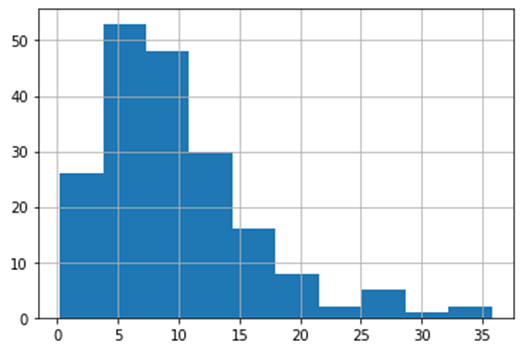
#Univariate histogram for suicide data:

seaborn.distplot(suicidedata['suicideper100th'].dropna(), kde=False);

plt.xlabel('Number of suicide per 100000')

plt.title('Number of countries Vs suicide per 100000 according to gapminder data')

#Univariate histogram for income data:

seaborn.distplot(incomedata['incomeperperson'].dropna(), kde=False);

plt.xlabel('Income per person')

plt.title('Number of countries Vs different income per person data')

#Univariate histogram for employment rate data:

seaborn.distplot(employratedata['employrate'].dropna(), kde=False);

plt.xlabel('Employment rate')

plt.title('Number of countries Vs different employment rate data')

#Univariate histogram for political score data:

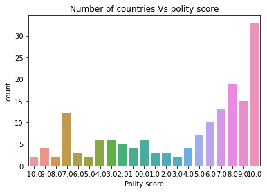
politydata['polityscore']= politydata['polityscore'].astype('category')

seaborn.countplot(x="polityscore", data=politydata);

plt.xlabel('Polity score')

plt.title('Number of countries Vs polity score')

#Plotting histograms of each variable

#Alternative way to generate histogram

plt.figure(figsize=(16,12))

plt.subplot(2,2,1)

plt.title('Suicide rate or suicideper100th')

suicidedata['suicideper100th'].hist(bins=10)

plt.subplot(2,2,2)

incomedata['incomeperperson'].hist(bins=10)

plt.title('Income per person')

plt.subplot(2,2,3)

employratedata['employrate'].hist(bins=10)

plt.title('Employment rate')

plt.subplot(2,2,4)

politydata['polityscore'].hist(bins=10)

plt.title('Political score or polityscore')

Discussion from univariate plots

It is quite clear from the univariate histogram plots that the number of suicide and income per person data is skewed left, employment rate data is unimodal and almost-normally distributed whereas the political score is skewed right. This means that the most of the countries have lower suicide rate and lower income data and only few countries have exceptionally high number for both these data. Employment rate is near-normal distribution meaning the data are spread uniformly about the mean center of the employment rate. Political score of most countries are more than the mean (which is zero). Hence, more countries have positive political score and there are lesser number of countries with negative political score.

#Binning and creating new category

#Categorizing countries in 5 different levels

bins = [0,1000,5000,10000,25000,300000]

group_names = ['Very poor,0-1000', 'Poor,1000-5000', 'Medium,5000-10000', 'Rich,10000-25000','Very rich,25000-300000']

categories = pandas.cut(incomedata['incomeperperson'], bins, labels=group_names)

incomedata['categories']= pandas.cut(incomedata['incomeperperson'], bins, labels=group_names)

pandas.value_counts(categories)

Output

Poor,1000-5000 61

Very poor,0-1000 54

Medium,5000-10000 28

Very rich,25000-300000 24

Rich,10000-25000 23

Name: incomeperperson, dtype: int64

#Bivariate plots

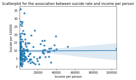
scat1 = seaborn.regplot(x="incomeperperson", y="suicideper100th", fit_reg=True, data=suicidedata)

plt.xlabel('Income per person')

plt.ylabel('Suicide per 100000')

plt.title('Scatterplot for the association between suicide rate and income per person')

# quartile split (use qcut function & ask for 4 groups - gives you quartile split)

print ('Income per person - 4 categories - quartiles')

incomedata['INCOMEGRP4']=pandas.qcut(incomedata.incomeperperson, 4, labels=["1=25th%tile","2=50%tile","3=75%tile","4=100%tile"])

c10 = incomedata['INCOMEGRP4'].value_counts(sort=False, dropna=True)

print(c10)

# bivariate bar graph C->Q

seaborn.catplot(x='INCOMEGRP4', y='suicideper100th', data=incomedata, kind="bar", ci=None)

plt.xlabel('income group')

plt.ylabel('Mean suicide rate')

c11= incomedata.groupby('INCOMEGRP4').size()

print (c11)

Output

Income per person - 4 categories - quartiles

1=25th%tile 48

2=50%tile 47

3=75%tile 47

4=100%tile 48

Name: INCOMEGRP4, dtype: int64

INCOMEGRP4

1=25th%tile 48

2=50%tile 47

3=75%tile 47

4=100%tile 48

dtype: int64

#Bivariate plot for suicide rate vs employment rate

scat2 = seaborn.regplot(x="employrate", y="suicideper100th", fit_reg=True, data=suicidedata)

plt.xlabel('Employment rate')

plt.ylabel('Suicide per 100000')

plt.title('Scatterplot for the association between suicide rate and employment rate')

#Bivariate C->Q plot for suicide rate vs political score

suicidedata["polityscore"] = suicidedata["polityscore"].astype('category')

seaborn.catplot(x="polityscore", y="suicideper100th", data=suicidedata, kind="bar", ci=None)

plt.xlabel('Polityscore')

plt.ylabel('Suicide per 100000')

plt.title('Categorical plot of suicide rate and political score')

# quartile split (use qcut function & ask for 4 groups - gives you quartile split)

politydata['polityscore4']=pandas.qcut(politydata.polityscore, 4, labels=["1=25th%tile","2=50%tile","3=75%tile","4=100%tile"])

c12 = politydata['polityscore4'].value_counts(sort=False, dropna=True)

print(c12)

# bivariate bar graph C->Q

seaborn.catplot(x='polityscore4', y='suicideper100th', data=politydata, kind="bar", ci=None)

plt.xlabel('political score grp')

plt.ylabel('Mean suicide rate')

c13= politydata.groupby('polityscore').size()

print (c13)

Output

1=25th%tile 42

2=50%tile 39

3=75%tile 47

4=100%tile 33

Name: polityscore4, dtype: int64

polityscore

-10.0 2

-9.0 4

-8.0 2

-7.0 12

-6.0 3

-5.0 2

-4.0 6

-3.0 6

-2.0 5

-1.0 4

0.0 6

1.0 3

2.0 3

3.0 2

4.0 4

5.0 7

6.0 10

7.0 13

8.0 19

9.0 15

10.0 33

dtype: int64

Discussion from bivariate plots

It is clear from the scatter plot that the income per person have almost no relationship with the suicide data. There is neither positive nor negative slope (the line seems to be almost horizontal). It is further confirmed by categorical bar chart as well. When income data was split into 4 categories, the mean suicide rate still didn’t show the clear trend. All the income categories had almost same mean suicide rate. Similar trend was seen for employment rate and political score as well.

0 notes

poudelbibek · 2 years ago

Text

Regression modeling Module 3 Assignment

Reminder (research problem and defined variables)

Study topic:

Primary topic

Suicide rate Vs. Income per person

Variables of interest:

incomeperperson: The data contains GDP per capita in US dollars divided by midyear population. This data is calculated adjusting the global inflation (without making deductions for the depreciation of fabricated assests or for depletion and degradation of natural resources). The data was provided by world bank.

Flow sequence for a python program

Steps:

Read the csv file.

Convert the datas of interest to numeric

Select only the readable data (exclude null or NaN)

Center the explanatory variable (by subtracting mean)

Merge the centered explanatory variable and response variable into a subset data

Fit Response variable vs. Explanatory variable into a linear regression model

Introduce other explanatory variable and Fit Response variable vs. Explanatory variable into a multiple regression model

Construct Q-Q plot, standardized residual plot, regression plot and leverage plot to evaluate the model fit

Python program

#Importing libraries

import numpy as np

import pandas as pandas

import statsmodels.api as sm

import statsmodels.formula.api as smf

import seaborn

import matplotlib.pyplot as plt

# bug fix for display formats to avoid run time errors

pandas.set_option('display.float_format', lambda x:'%.2f'%x)

#Reading the data csv file

data = pandas.read_csv('gapminder.csv')

### Suiciderate is response whereas incomeperperson is explanatory variable

#setting variables of interest to numeric and creating datasets for response and explanatory variables

data['suicideper100th'] = pandas.to_numeric(data['suicideper100th'],errors = 'coerce')

data['incomeperperson'] = pandas.to_numeric(data['incomeperperson'],errors = 'coerce')

data['employrate'] = pandas.to_numeric(data['employrate'],errors = 'coerce')

data['polityscore'] = pandas.to_numeric(data['polityscore'],errors = 'coerce')

#Subset for data of interest

dataofinterest = data[['country','incomeperperson','suicideper100th' ,'employrate','polityscore']]

#Filtering countries with valid suicidedata and incomeperpersondata

suicidedata = dataofinterest[dataofinterest['suicideper100th'].notna()].suicideper100th

incomedata = dataofinterest[dataofinterest['incomeperperson'].notna()].incomeperperson

employratedata = dataofinterest[dataofinterest['employrate'].notna()].employrate

politydata = dataofinterest[dataofinterest['polityscore'].notna()].polityscore

#Center the explanatory variable i.e. incomeperperson

center_function = lambda politydata: politydata - politydata.mean()

politydata_centered = center_function(politydata)

print(politydata_centered.mean())

Output (Mean of centered polityscore_centered): - 3.91681166451608e-16

#Integrating data of interests with centered explanatory variable

di = pandas.DataFrame(data['country'])

#Merge centered income data and suicide data into new dataframe

di = pandas.concat([di,incomedata,suicidedata,employratedata,politydata_centered],axis=1)

##Basic linear regression

reg1 = smf.ols('suicideper100th ~ incomeperperson',data=di).fit()

print(reg1.summary())

Output:

OLS Regression Results

==============================================================================

Dep. Variable: suicideper100th R-squared: 0.000

Model: OLS Adj. R-squared: -0.006

Method: Least Squares F-statistic: 0.007692

Date: Fri, 24 Feb 2023 Prob (F-statistic): 0.930

Time: 18:05:50 Log-Likelihood: -586.59

No. Observations: 181 AIC: 1177.

Df Residuals: 179 BIC: 1184.

Df Model: 1

Covariance Type: nonrobust

===================================================================================

coef std err t P>|t| [0.025 0.975]

-----------------------------------------------------------------------------------

Intercept 9.6483 0.543 17.767 0.000 8.577 10.720

incomeperperson 3.237e-06 3.69e-05 0.088 0.930 -6.96e-05 7.61e-05

==============================================================================

Omnibus: 53.138 Durbin-Watson: 2.089

Prob(Omnibus): 0.000 Jarque-Bera (JB): 108.474

Skew: 1.370 Prob(JB): 2.79e-24

Kurtosis: 5.622 Cond. No. 1.73e+04

==============================================================================

Warnings:

[1] Standard Errors assume that the covariance matrix of the errors is correctly specified.

[2] The condition number is large, 1.73e+04. This might indicate that there are

strong multicollinearity or other numerical problems.

Linear regression eqn: Suicideper100th = 9.6483 + 3.237*10^-6 * incomeperperson

P-value: 0.93 (higher than α -statistically not significant)

R2 = 0.00 (very weak fit of a model)

#Multiple regression model

reg3 = smf.ols('suicideper100th ~ incomeperperson + I(incomeperperson**2) + employrate + polityscore',data=di).fit()

print(reg3.summary())

OLS Regression Results

==============================================================================

Dep. Variable: suicideper100th R-squared: 0.023

Model: OLS Adj. R-squared: -0.004

Method: Least Squares F-statistic: 0.8568

Date: Fri, 24 Feb 2023 Prob (F-statistic): 0.492

Time: 18:05:51 Log-Likelihood: -494.67

No. Observations: 152 AIC: 999.3

Df Residuals: 147 BIC: 1014.

Df Model: 4

Covariance Type: nonrobust

===========================================================================================

coef std err t P>|t| [0.025 0.975]

-------------------------------------------------------------------------------------------

Intercept 8.7690 3.320 2.641 0.009 2.208 15.330

incomeperperson -0.0002 0.000 -0.786 0.433 -0.001 0.000

I(incomeperperson ** 2) 4.213e-09 5.74e-09 0.734 0.464 -7.14e-09 1.56e-08

employrate 0.0279 0.053 0.530 0.597 -0.076 0.132

polityscore 0.1456 0.088 1.658 0.099 -0.028 0.319

==============================================================================

Omnibus: 47.889 Durbin-Watson: 2.080

Prob(Omnibus): 0.000 Jarque-Bera (JB): 96.798

Skew: 1.420 Prob(JB): 9.56e-22

Kurtosis: 5.687 Cond. No. 2.27e+09

==============================================================================

Discussion: Even though R2 increased to 0.023 it is still a very weak model fit. The p values for all the variables (incomeperperson, incomeperperson**2, employrate, and polityscore) are above the significance level. This means that all the variables are statistically insignificant.

Confidence intervals:

#Q-Q plot

fig1=sm.qqplot(reg3.resid, line='r')

Q-Q plot clearly shows how poor the model is. The model is especially worse when the explanatory variables are very high or very low.

#Standardized residual plot

stdres = pandas.DataFrame(reg3.resid_pearson)

fig2 = plt.plot(stdres,'o',ls='None')

l = plt.axhline(y=0, color = 'r')

plt.ylabel('Standardized Residual')

plt.xlabel('Observation Number')

print(fig2)

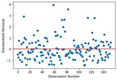
Discussion: The standardized residual plot clearly shows that the couple of data above three standard deviations away (meaning they are outliers). Also there are many datas above 2.5 standard deviations away meaning the model is a poor fit. There are however no data on the lower bound meaning there are no data below -2 standard deviations away.

#Regression plots for incomeperperson

fig3 = plt.figure(figsize=(12,8))

fig3 = sm.graphics.plot_regress_exog(reg3,"incomeperperson",fig=fig3)

Discussion: The residuals are significantly high when the income values are lower. Partial regression plot shows there is significant prediction error.

#Leverage plot

fig5 = sm.graphics.influence_plot(reg3,size = 8)

print(fig5)

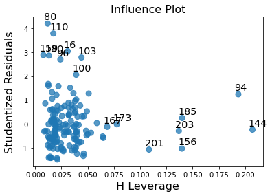
Discussion: Similar to standard residual plot, leverage plot also shows there are some outliers above 2 but not below -2. However, the outliers above 2 are of smaller significance or influence. The data with high leverage are not seen to be outliers.

0 notes

poudelbibek · 2 years ago

Text

Data management and visualization Module 3 Assignment

Data visualization Assignment 3

Reminder (research problem and defined variables)

Study topic:

Primary topic

Suicide rate Vs. various socio-economic reasons (income per person/ employment rate/ country’s political score)

Variables of interest:

Python program

import pandas

import numpy as np

import matplotlib.pyplot as plt

# any additional libraries would be imported here

#Reading data

data = pandas.read_csv('gapminder_data.csv', low_memory=False)

print (len(data)) #number of observations (rows)

print (len(data.columns)) # number of variables (columns)

213

#Assuring data collected is what we want

data.head()

#setting variables of interest to numeric

data['suicideper100th'] = pandas.to_numeric(data['suicideper100th'],errors = 'coerce')

data['employrate'] = pandas.to_numeric(data['employrate'],errors = 'coerce')

data['polityscore'] = pandas.to_numeric(data['polityscore'],errors = 'coerce')

data['incomeperperson'] = pandas.to_numeric(data['incomeperperson'],errors = 'coerce')

#Coding out missing data or Filtering countries with valid data for various variables

#Filtering countries with valid suicidedata

suicidedata = data[data['suicideper100th'].notna()]

Num_suicidedata = len(suicidedata)

print('Number of countries with available suicide data:', Num_suicidedata)

print('Number of countries with missing suiciderate data:', len(data)-Num_suicidedata)

#Filtering countries with valid employment rate data

employratedata = data[data['employrate'].notna()]

Num_employratedata = len(employratedata)

print('Number of countries with available employment rate data:', Num_employratedata)

print('Number of countries with missing employment rate data:', len(data)-Num_employratedata)

#Filtering countries with valid income data

incomedata = data[data['incomeperperson'].notna()]

Num_incomedata = len(incomedata)

print('Number of countries with available incomeperperson data:', Num_incomedata)

print('Number of countries with missing incomeperperson data:', len(data)-Num_incomedata)

#Filtering countries with valid political score data

politydata = data[data['polityscore'].notna()]

Num_politydata = len(politydata)

print('Number of countries with available political score data:', Num_politydata)

print('Number of countries with missing political score data:', len(data)-Num_politydata)

Output

Number of countries with available suicide data: 191

Number of countries with missing suiciderate data: 22

Number of countries with available employment rate data: 178

Number of countries with missing employment rate data: 35

Number of countries with available incomeperperson data: 190

Number of countries with missing incomeperperson data: 23

Number of countries with available political score data: 161

Number of countries with missing political score data: 52

#Binning variables and creating frequency tables

#Separate variables 10 levels and count the frequency

suiciderate_bins = pandas.cut(suicidedata['suicideper100th'], bins = np.linspace(0,40,num=11))

suiciderate_bins.value_counts(sort=False, dropna=False)

Output

(0.0, 4.0] 27

(4.0, 8.0] 61

(8.0, 12.0] 50

(12.0, 16.0] 31

(16.0, 20.0] 8

(20.0, 24.0] 6

(24.0, 28.0] 4

(28.0, 32.0] 2

(32.0, 36.0] 2

(36.0, 40.0] 0

Name: suicideper100th, dtype: int64

incomeperperson_bins = pandas.cut(incomedata['incomeperperson'], bins = np.linspace(0,110000,num=12))

incomeperperson_bins.value_counts(sort=False, dropna=False)

Output:

(0.0, 10000.0] 143

(10000.0, 20000.0] 17

(20000.0, 30000.0] 14

(30000.0, 40000.0] 12

(40000.0, 50000.0] 0

(50000.0, 60000.0] 1

(60000.0, 70000.0] 1

(70000.0, 80000.0] 0

(80000.0, 90000.0] 1

(90000.0, 100000.0] 0

(100000.0, 110000.0] 1

Name: incomeperperson, dtype: int64

employrate_bins = pandas.cut(employratedata['employrate'], bins = np.linspace(0,100,num=11))

employrate_bins.value_counts(sort=False, dropna=False)

Output

(0.0, 10.0] 0

(10.0, 20.0] 0

(20.0, 30.0] 0

(30.0, 40.0] 5

(40.0, 50.0] 32

(50.0, 60.0] 67

(60.0, 70.0] 47

(70.0, 80.0] 21

(80.0, 90.0] 6

(90.0, 100.0] 0

Name: employrate, dtype: int64

#For polityscore as it is already discretized from -10 to to, it's not required to bin

data['polityscore'].value_counts(sort=False, dropna=False)

Output

0.0 6

9.0 15

2.0 3

NaN 52

-2.0 5

8.0 19

5.0 7

10.0 33

-7.0 12

7.0 13

3.0 2

6.0 10

-4.0 6

-1.0 4

-3.0 6

-5.0 2

1.0 3

-6.0 3

-9.0 4

4.0 4

-8.0 2

-10.0 2

Name: polityscore, dtype: int64

#Plotting histograms of each variable

plt.figure(figsize=(16,12))

plt.subplot(2,2,1)

plt.title('Suicide rate or suicideper100th')

suicidedata['suicideper100th'].hist(bins=10)

plt.subplot(2,2,2)

incomedata['incomeperperson'].hist(bins=10)

plt.title('Income per person')

plt.subplot(2,2,3)

employratedata['employrate'].hist(bins=10)

plt.title('Employment rate')

plt.subplot(2,2,4)

politydata['polityscore'].hist(bins=10)

plt.title('Political score or polityscore')

Output

Summary of histogram results:

Suicideper100th – Lots of countries seem to have suicide rate between 5-15 per 100,000. There are very few countries which reported the amount of suicide more than 20 per 100,000 deaths.

Incomeperperson – Around 140 countries have their income per person ranging from 0-10000. The countries with income per person higher than 40000 are extremely few.

Employrate – Employment rate data actually had a near-nominal distribution. There are few countries with low employment rate (around 30) and some countries with very high employment rate (around 90) but majority of them are between 40-70 with mean being around 55-60 %.

Polityscore – The histogram plot shows that many countries in the world are actually democratic and have higher freedom of speech. Around 70 countries have political score more than 7.5. Sadly, there are still countries with -10 polityscore as well.

#Categorizing countries in 5 different levels

bins = [0,1000,5000,10000,25000,300000]

group_names = ['Very poor,0-1000', 'Poor,1000-5000', 'Medium,5000-10000', 'Rich,10000-25000','Very rich,25000-300000']

categories = pandas.cut(incomedata['incomeperperson'], bins, labels=group_names)

incomedata['categories']= pandas.cut(incomedata['incomeperperson'], bins, labels=group_names)

pandas.value_counts(categories)

Output

Poor,1000-5000 61

Very poor,0-1000 54

Medium,5000-10000 28

Very rich,25000-300000 24

Rich,10000-25000 23

Name: incomeperperson, dtype: int64

#Creating subset data of countries of 5 different income levels

Veryrichcountries = incomedata[incomedata['categories']=='Very rich,25000-300000']

Richcountries = incomedata[incomedata['categories']=='Rich,10000-25000']

Mediumcountries = incomedata[incomedata['categories']=='Medium,5000-10000']

Poorcountries = incomedata[incomedata['categories']=='Poor,1000-5000']

Verypoorcountries = incomedata[incomedata['categories']=='Very poor,0-1000']

#Average of suicide rate of different categorical countries

print('The average suicide rate of very rich countries is:',Veryrichcountries['suicideper100th'].mean())

print('The average suicide rate of rich countries is:',Richcountries['suicideper100th'].mean())

print('The average suicide rate of medium countries is:',Mediumcountries['suicideper100th'].mean())

print('The average suicide rate of poor countries is:',Poorcountries['suicideper100th'].mean())

print('The average suicide rate of very poor countries is:',Verypoorcountries['suicideper100th'].mean())

Output

The average suicide rate of very rich countries is: 10.369718011599998

The average suicide rate of rich countries is: 7.746234288666666

The average suicide rate of medium countries is: 10.028339147740738

The average suicide rate of poor countries is: 9.534145223233335

The average suicide rate of very poor countries is: 10.150774681113209

0 notes

poudelbibek · 2 years ago

Text

Data management and visualization Module 2 Assignment

Reminder (research problem and defined variables)

Study topic:

Primary topic

Suicide rate Vs. various socio-economic reasons (income per person/ employment rate/ country’s political score)

Variables of interest:

incomeperperson: The data contains GDP per capita in US dollars divided by midyear population. This data is calculated adjusting the global inflation (without making deductions for the depreciation of fabricated assests or for depletion and degradation of natural resources). The data was provided by world bank.

employrate: This data provides the percentage of total population of age group (above 15) that has been employed during the given year. This data was provided by International labour organization.

Python program

#Importing libraries

import pandas

import numpy

# any additional libraries would be imported here

#Reading data

data = pandas.read_csv('gapminder_data.csv', low_memory=False)

print (len(data)) #number of observations (rows)

print (len(data.columns)) # number of variables (columns)

#Assuring data collected is what we want

data.head()

#Number of countries

Num_countries = len(data)

print(Num_countries)

#Number of parameters

Num_parameters = data.shape[1] #0 for rows 1 for columns using shape command

print(Num_parameters)

#setting variables of interest to numeric

###

data['suicideper100th'] = pandas.to_numeric(data['suicideper100th'],errors = 'coerce')

data['employrate'] = pandas.to_numeric(data['employrate'],errors = 'coerce')

data['polityscore'] = pandas.to_numeric(data['polityscore'],errors = 'coerce')

data['incomeperperson'] = pandas.to_numeric(data['incomeperperson'],errors = 'coerce')

###

#Filtering countries with valid suicidedata

suicidedata = data[data['suicideper100th'].notna()]

Num_suicidedata = len(suicidedata)

print(Num_suicidedata)

#Filtering countries with valid employment rate data

employratedata = data[data['employrate'].notna()]

Num_employratedata = len(employratedata)

print(Num_employratedata)

#Filtering countries with valid income data

incomedata = data[data['incomeperperson'].notna()]

Num_incomedata = len(incomedata)

print(Num_incomedata)

#Filtering countries with valid political score data

politydata = data[data['polityscore'].notna()]

Num_politydata = len(politydata)

print(Num_politydata)

#Highest and lowest data of every parameter

Highest_income = incomedata['incomeperperson'].max()

Lowest_income = incomedata['incomeperperson'].min()

print('Highest income = {0:0.2f} and Lowest income = {1:0.2f}'.format(Highest_income,Lowest_income))

Highest income = 105147.44 and Lowest income = 103.78

Highest_employrate = employratedata['employrate'].max()

Lowest_employrate = employratedata['employrate'].min()

print('Highest employment rate = {0:0.2f} and Lowest employment rate = {1:0.2f}'.format(Highest_employrate,Lowest_employrate)) Highest employment rate = 83.20 and Lowest employment rate = 32.00

Highest_polityscore = politydata['polityscore'].max()

Lowest_polityscore = politydata['polityscore'].min()

print('Highest polityscore = {0:0.2f} and Lowest polityscore = {1:0.2f}'.format(Highest_polityscore,Lowest_polityscore))

Highest polityscore = 10.00 and Lowest polityscore = -10.00

Highest_suiciderate = suicidedata['suicideper100th'].max()

Lowest_suiciderate = suicidedata['suicideper100th'].min()

print('Highest suicide rate = {0:0.2f} and Lowest suicide rate = {1:0.2f}'.format(Highest_suiciderate,Lowest_suiciderate))

Highest suicide rate = 35.75 and Lowest suicide rate = 0.20

#Frequency tables

#Separate variables 10 levels and count the frequency

suiciderate_bins = pandas.cut(suicidedata['suicideper100th'], bins = np.linspace(0,40,num=11))

suiciderate_bins.value_counts(sort=False, dropna=False)

(0.0, 4.0] 27

(4.0, 8.0] 61

(8.0, 12.0] 50

(12.0, 16.0] 31

(16.0, 20.0] 8

(20.0, 24.0] 6

(24.0, 28.0] 4

(28.0, 32.0] 2

(32.0, 36.0] 2

(36.0, 40.0] 0

Name: suicideper100th, dtype: int64

incomeperperson_bins = pandas.cut(incomedata['incomeperperson'], bins = np.linspace(0,110000,num=12))

incomeperperson_bins.value_counts(sort=False, dropna=False)

(0.0, 10000.0] 143

(10000.0, 20000.0] 17

(20000.0, 30000.0] 14

(30000.0, 40000.0] 12

(40000.0, 50000.0] 0

(50000.0, 60000.0] 1

(60000.0, 70000.0] 1

(70000.0, 80000.0] 0

(80000.0, 90000.0] 1

(90000.0, 100000.0] 0

(100000.0, 110000.0] 1

employrate_bins = pandas.cut(employratedata['employrate'], bins = np.linspace(0,100,num=11))

employrate_bins.value_counts(sort=False, dropna=False)

(0.0, 10.0] 0

(10.0, 20.0] 0

(20.0, 30.0] 0

(30.0, 40.0] 5

(40.0, 50.0] 32

(50.0, 60.0] 67

(60.0, 70.0] 47

(70.0, 80.0] 21

(80.0, 90.0] 6

(90.0, 100.0] 0

Name: employrate, dtype: int64

#For polityscore as it is already discretized from -10 to to, it's not required to bin

data['polityscore'].value_counts(sort=False, dropna=False)

-1 4

10 33

-6 3

1 3

9 15

5 7

3 2

-4 6

-5 2

6 10

4 4

-8 2

7 13

-7 12

2 3

-3 6

8 19

-10 2

-2 5

0 6

-9 4

Name: polityscore, dtype: int64

#Plotting histograms of each variable

suicidedata['suicideper100th'].hist(bins=10)

incomedata['incomeperperson'].hist(bins=10)

employratedata['employrate'].hist(bins=10)

politydata['polityscore'].hist(bins=10)

Summary of findings:

There is a data of 213 countries.

Missing data for various parameters

suicideper100th – The given dataset presents suicide data for 191 countries meaning 22 countries data is missing.

Employrate – 178 countries data found, 35 countries missing

Incomeperperson – 190 countries data found, 23 countries missing

Polityscore – 161 countries data found, 52 countries missing

Highest and lowest data:

Suicideper100th - Highest suicide rate = 35.75 and Lowest suicide rate = 0.20

Incomeperperson - Highest income = 105147.44 and Lowest income = 103.78

Employrate - Highest employment rate = 83.20 and Lowest employment rate = 32.00

Polityscore - Highest polityscore = 10.00 and Lowest polityscore = -10.00

Frequency table:

Suicideper100th

(0.0, 4.0] 27

(4.0, 8.0] 61

(8.0, 12.0] 50

(12.0, 16.0] 31

(16.0, 20.0] 8

(20.0, 24.0] 6

(24.0, 28.0] 4

(28.0, 32.0] 2

(32.0, 36.0] 2

(36.0, 40.0] 0

Incomeperperson

(0.0, 10000.0] 143

(10000.0, 20000.0] 17

(20000.0, 30000.0] 14

(30000.0, 40000.0] 12

(40000.0, 50000.0] 0

(50000.0, 60000.0] 1

(60000.0, 70000.0] 1

(70000.0, 80000.0] 0

(80000.0, 90000.0] 1

(90000.0, 100000.0] 0

(100000.0, 110000.0] 1

Employrate:

0.0, 10.0] 0

(10.0, 20.0] 0

(20.0, 30.0] 0

(30.0, 40.0] 5

(40.0, 50.0] 32

(50.0, 60.0] 67

(60.0, 70.0] 47

(70.0, 80.0] 21

(80.0, 90.0] 6

(90.0, 100.0] 0

Polityscore

-1 4

10 33

Missing 52

-6 3

1 3

9 15

5 7

3 2

-4 6

-5 2

6 10

4 4

-8 2

7 13

-7 12

2 3

-3 6

8 19

-10 2

-2 5

0 6

-9 4

Summary of histogram results:

Suicideper100th – Lots of countries seem to have suicide rate between 5-15 per 100,000. There are very few countries which reported the amount of suicide more than 20 per 100,000 deaths.

Incomeperperson – Around 140 countries have their income per person ranging from 0-10000. The countries with income per person higher than 40000 are extremely few.

0 notes

poudelbibek · 2 years ago

Text

Regression Modeling in Practice Module 2 Assignment

Regression modeling Assignment 2

Reminder (research problem and defined variables)

Study topic:

Primary topic

Suicide rate Vs. Income per person

Variables of interest:

Flow sequence for a python program

Steps:

Read the csv file.

Convert the data of interest to numeric.

Select only the readable data (exclude null or NaN).

Center the explanatory variable by subtracting mean (however not needed on the explanatory variable we have chosen).

Merge the centered explanatory variable and response variable into a subset data.

Scatterplot the Response variable vs. Explanatory variable.

Fit Response variable vs. Explanatory variable into a linear regression model.

Python program

#Importing libraries

import numpy as np

import pandas as pandas

import statsmodels.api

import statsmodels.formula.api as smf

import seaborn

import matplotlib.pyplot as plt

# bug fix for display formats to avoid run time errors

pandas.set_option('display.float_format', lambda x:'%.2f'%x)

#Reading the data csv file

data = pandas.read_csv('gapminder.csv')

### Suiciderate is response whereas incomeperperson is explanatory variable

#setting variables of interest to numeric and creating datasets for response and explanatory variables

data['suicideper100th'] = pandas.to_numeric(data['suicideper100th'],errors = 'coerce')

data['incomeperperson'] = pandas.to_numeric(data['incomeperperson'],errors = 'coerce')

#Subset for data of interest

dataofinterest = data[['country','incomeperperson','suicideper100th']]

#Filtering countries with valid suicidedata and incomeperpersondata

suicidedata = dataofinterest[dataofinterest['suicideper100th'].notna()].suicideper100th

incomedata = dataofinterest[dataofinterest['incomeperperson'].notna()].incomeperperson

###This step is not needed

#Mean of income data

print(incomedata.mean())

Output (Mean of actual explanatory variable): 8740.966

#Center the explanatory variable i.e. incomeperperson

center_function = lambda incomedata: incomedata - incomedata.mean()

incomedata_centered = center_function(incomedata)

print(incomedata_centered.mean())

Output (Mean of centered explanatory variable): -3.934761288722879e-12

(The mean is very small,close to 0, meaning that the centering has been properly executed)

#Integrating data of interests with centered explanatory variable

di = pandas.DataFrame(data['country'])

#Merge centered income data and suicide data into new dataframe

di = pandas.concat([di,incomedata,suicidedata],axis=1)

##Basic linear regression

#Scatterplot

s1 = seaborn.regplot(x="incomeperperson", y = "suicideper100th", scatter = True, data=di)

plt.xlabel('Incomeperperson_Centered')

plt.ylabel('Suicideper100th')

plt.title('Scatterplot for association between suicide rate and income per person')

print (s1)

#Linear regression model

reg1 = smf.ols('suicideper100th ~ incomeperperson',data=di).fit()

print(reg1.summary())

OLS Regression Results

==============================================================================

Dep. Variable: suicideper100th R-squared: 0.000

Model: OLS Adj. R-squared: -0.006

Method: Least Squares F-statistic: 0.007692

Date: Sun, 19 Feb 2023 Prob (F-statistic): 0.930

Time: 22:35:18 Log-Likelihood: -586.59

No. Observations: 181 AIC: 1177.

Df Residuals: 179 BIC: 1184.

Df Model: 1

Covariance Type: nonrobust

===================================================================================

coef std err t P>|t| [0.025 0.975]

-----------------------------------------------------------------------------------

Intercept 9.6483 0.543 17.767 0.000 8.577 10.720

incomeperperson 3.237e-06 3.69e-05 0.088 0.930 -6.96e-05 7.61e-05

==============================================================================

Omnibus: 53.138 Durbin-Watson: 2.089

Prob(Omnibus): 0.000 Jarque-Bera (JB): 108.474

Skew: 1.370 Prob(JB): 2.79e-24

Kurtosis: 5.622 Cond. No. 1.73e+04 ==============================================================================

Warnings:

[1] Standard Errors assume that the covariance matrix of the errors is correctly specified.

[2] The condition number is large, 1.26e+04. This might indicate that there are

strong multicollinearity or other numerical problems.

Discussion from regression results:

The regression analysis provided multiple insight of the data and the association between our response variable (suicide rate) and explanatory variable (income per person). First of all, the R2 value was seen to be 0.000 which indicated that the fitted line was an extremely bad fit meaning there was no linear relationship between explanatory and response variable. This can also be seen from the scatter plot which clearly shows huge deviations of actual data from the fitted line.

The regression coefficients were:

Intercept = 9.6483

slope (of incomeperpeson) = 3.237e-6

It means that for every 1 step change in income per person, the change in suicideper100th will be 3.237e-6.

Importantly, the key observation from the data was even though income per person was supposed to have a significant association with the suicide rate, the p value being 0.93 (p=0.93) showed that the relation between income per person and suicide rate was not statistically significant.

From the omnibus and Jarque-Bera test, we saw that the prob (omnibus) and Prob(JB) were 0 and 2.79e-24 which is extremely low. This signifies that our data was clearly not distributed normally. The assumption of normal distribution in linear regression modeling is, hence, not true for this dataset. From the scatter plot, we can observe that the assumption of homoscedasticity was also not met by this dataset. The deviation of data from the fitted line is of inconstant variance.

0 notes

poudelbibek · 2 years ago

Text

Regression Modeling in Practice Module 1 Assignment

Research data to be studied: Suicide rate per 100,000 people in different countries

Sample:

The dataset that would be used in the study will be the Gapminder dataset. Gapminder collects a data from various reliable sources such as World Health Organization (WHO), International labor organization (ILO), World Bank, etc. The suicide rate per 100,000 population data was based on combination of time series from WHO Violence and Injury Prevention (VIP) and data from WHO Global Burden of Disease 2002 and 2004. The data is collected from 192 UN listed countries and 21 additional different areas giving a total of 213 (N=213) data sets as the geographic areas. The data consists of record for different genders and age groups.

Procedure:

The presented data is a country-level surveillance data collected by different government and international agencies in different areas during 2002-2004. Since suicide data was recorded by each country or a region, those data were drawn by WHO and was ultimately collected by Gapminder from the WHO database. As mentioned earlier, the suicide rate per 100,000 population data was collected via different sources in 2002 and 2004 from 192 UN listed countries and 21 additional different areas giving a total of 213 (N=213) data sets as the geographic areas. The purpose of this study was to figure out the suicide rate of any country and how it is affected by other causes.

Methods:

Deaths recorded in this data strictly only consists of the mortality data due to self-inflicted injury. The assessment of whether the death falls into accident or self-harm was done by health agencies before categorizing them. Also, this data was age adjusted which means that the reported rate is computed using the direct method by applying age-specific rates in a population of interest to a standardized age distribution. This eliminates differences in observed rates that result from age differences in population composition. The suicide rate here is the response variable. What we are interested are the causes on what is affecting the suicide rate. Hence, I am interested in how the income of a person, employment rate and the political score of a country affects the suicide rate. Suicide rate was recorded per 100,000 population in any given country whereas income per person is an average income of a person per annum and employment rate is based on percentage of total population that are currently employed. Political score is based on the democratic score of a country. It ranged from -10 to 10 where -10 represents a country with autocratic government whereas value 10 was assigned to a liberal country with high freedom of speech. Various linear regression models and dependency plots will be generated to study the association of various causes to the suicide rate.

0 notes

poudelbibek · 2 years ago

Text

Data Management and Visualization Module 1 Assignment

Dataset:

I chose the gapminder dataset for my project. I am interested in socio-economic data of different countries.

Study topic:

Primary topic

I am highly interested in knowing about suicide rate of different countries and how they are being affected by various socio-economic reasons.

In particular, I want to study the dependency of suicide rate with two different economic factors: income per person and employment rate. The questions I would be exploring are:

Is the suicide rate affected by income per person?

Is higher unemployment rate associated with higher suicide rate?

Secondary topic

In addition, I am also interested not only in the economic reason but the social reason as well for high suicide rate in any country. So, the secondary question that I will be asking is:

How much does a country’s democracy score (free nature) affect the suicide rate of that country?

Personalized codebook:

Adapted from the gapminder codebook, I have down-selected the following parameters as a part of my study:

incomeperperson: The data contains GDP per capita in US dollars divided by midyear population. This data is calculated adjusting the global inflation (without making deductions for the depreciation of fabricated assests or for depletion and degradation of natural resources). The data was provided by world bank.

employrate: This data provides the percentage of total population of age group (above 15) that has been employed during the given year. This data was provided by International labour organization.

Literature review:

Suicide has been a topic of intriguing study across many countries. Various research has been conducted to determine cause of suicide [1-6]. Suicides are most commonly associated with low income, family stress, alcohol consumption, relationship issues, career failures and many other socio-economic issues. Ying and Chang [1] reported that a low income family with an unemployed man/woman is at high risk for adult male suicide. Similarly, Chen et al. [2] accounted family conflicts and job unavailability as major perpetrators for suicide [2]. Similarly, the nature of job has also been pinpointed by several study as a cause for depression in many people. For example, farming all across the world is one of the low-income job and that has been accounted as a reason for a spike in suicide among farmers in many countries [3]. Hence, the correlation between income per person and employment rate with suicide rate was chosen for this statistical study.

More interestingly, there are several studies on effect of political climate on suicide rate of the particular country [4-6]. Politically, the weight of the evidence suggests that laws increasing social welfare expenditures and other policies assisting persons with low incomes (e.g., minimum wage) tend to lower suicide rates [4]. Flavin and Radcliff [5] reported that general state policy liberalism and the governing ideologies of state governments are linked to suicide rates as well. Also, sadly the news of suicide bombers with some political ideologies often are heard in the news [6]. So, study on effect of political score of a country on suicide rate would be another interesting statistical study.

Hypothesis:

Economic condition is the biggest factor to lead people to clinical depression (and ultimately suicide). Hence, a hypothesis is made that the higher the income per person and employment rate is, lower the suicide rate will be. Another reason for suicide is a political reason. Most of the people want to be politically free and have their freedom of speech. Autocratic state and restricting people on their speech might also lead to depression and a feeling to hurt oneself. National policies and regulations might dictate how people react to a crisis: be that social or financial. Hence, the country with higher positive polity score has been hypothesized to have lower suicide rate.

References

[1] Ying, Yung-hsiang, and Koyin Chang. "A study of suicide and socioeconomic factors." Suicide and life-threatening behavior 39, no. 2 (2009): 214-226.

[2] Chen, Ying-Yeh, Kevin Chien-Chang Wu, Saman Yousuf, and Paul SF Yip. "Suicide in Asia: opportunities and challenges." Epidemiologic reviews 34, no. 1 (2012): 129-144.

[3] Behere, Prakash B., and Manik C. Bhise. "Farmers' suicide: Across culture." Indian Journal of psychiatry 51, no. 4 (2009): 242.

[4] Stack, Steven. "Contributing factors to suicide: Political, social, cultural and economic." Preventive medicine 152 (2021): 106498.

[5] Flavin, Patrick, and Benjamin Radcliff. "Public policies and suicide rates in the American states." Social Indicators Research 90, no. 2 (2009): 195-209.

[6] Soibelman, Mali. "Palestinian suicide bombers." Journal of investigative psychology and offender profiling 1, no. 3 (2004): 175-190.

1 note · View note