razorvision-blog - Tumblr blog

razorvision-blog · 13 years

Text

How to Compile RGBDemo 0.6.1

Introduction

RGBDemo is computer vision software in C++ for Kinect.

The software library includes an app (the reconstructor), which builds 3D models quickly and easily as you move the kinect around a room.

Prerequisites:

This tutorial is for Windows (specifically, I’m using windows 7).

Kinect and Software/Drivers. If you don’t have a Kinect or haven’t installed OpenNI, you should check out one of my first tutorials for details. Here is one that explains the Kinect prerequisites and how to install the software required: http://razorvision.tumblr.com/post/14221437255/compiling-the-open-source-kinect-fusion-pcl-point

Visual Studio 2008 or 2010 (I use 2010 in the tutorial)

32 vs. 64 bit

I recommend that you use 32 bit everything until the kinks are worked out with 64 bit.

Install OpenNI

If you have installed PCL through the all-in-one installer, then you'll need to uninstall the version of OpenNI that it installed. Do that first from the windows control panel before continuing.

Go to the OpenNI website at:

http://www.openni.org/

At the top, click Downloads --> OpenNI Modules

From the drop down, select OpenNI Binaries.

From the second drop down, then select "Unstable"

Finally, select the correct version for your operating system and 32-bit or 64-bit.

Click download and then install it.

Install OpenNI Nite

Go to the OpenNI website at:

http://www.openni.org/

At the top, click Downloads --> OpenNI Modules

From the drop down, select OpenNI Compliant Middleware Binaries.

From the second drop down, then select "Unstable"

Finally, select the correct version for your operating system and 32-bit or 64-bit.

Click download and then install it.

Download the Source Code

Download the latest version of RGBDemo from

https://github.com/nburrus/rgbdemo

Click the “zip” link: https://github.com/nburrus/rgbdemo/zipball/master

download it to the folder: C:\RGBDemo-0.6.1-git

Extract the contents there such that the folder calibration is at location:

C:\RGBDemo-0.6.1-git\calibration

Also download the Nestk source code, which is the base library for all this code. The demo depends on it.

Go to https://github.com/nburrus/nestk

And click the “Zip” link:

https://github.com/nburrus/nestk/zipball/master

Extract the contents of the download to the folder

C:\RGBDemo-0.6.1-git\nestk

Such that the “cmake” folder is located at:

C:\RGBDemo-0.6.1-git\nestk\cmake

Compile QT for Visual Studio 2010 if Necessary

If you are using Visual Studio 2010, you’ll need to follow the instructions here:

Download the QT source code from:

http://get.qt.nokia.com/qt/source/qt-everywhere-opensource-src-4.7.3.zip

After installing QT, you will need to compile it using the Visual Studio 2010 Command Prompt

This is located at Start --> All Programs --> Microsoft Visual Studio 2010 --> Visual Studio Tools -->

Visual Studio Command Prompt (2010)

Open that and then navigate to c:\qt\4.7.4

Type (without the quotes) into the command prompt.

configure -release -no-webkit -no-phonon -no-phonon-backend -no-script -no-scripttools -no-qt3support -no-multimedia -no-ltcg

Hit Enter

Next, type nmake after it is all done configuring.

This will take a while! Maybe 30 minutes.

If you need more help configuring this properly. You can see the original article on how to do it here:

http://stackoverflow.com/questions/5601950/how-to-build-qt-for-visual-studio-2010

Now add QT’s bin folder to the path.

For me, I went to: Start --> Right Click Computer --> Click Properties --> Click Advanced System Settings on the left side --> Click Environment Variables near the bottom right --> Go to the second section of the window that opened under “System Variables”. Scroll to the “Path” variable and click edit.

Add an extra semicolon to the end of the value and then append the path: C:\Qt\4.7.4\bin

Click ok on both windows. That’s all!

Configure Source Code With CMake GUI

If you haven’t already, download and install CMake GUI.

Open CMake GUI. Set the source directory (the first textbox) to C:/RGBDemo-0.6.1-git

Set the build directory (the second textbox) to C:/RGBDemo-0.6.1-git/build

Click the file menu and then click “Delete Cache” just in case to make sure CMake doesn’t screw up from previous projects you’ve used it with.

Click the Configure button

Choose your compiler and click ok. I chose Visual Studio 2010 Win64.

OpenCV

If you haven’t downloaded and installed OpenCV, do so. You’ll need at least version 2.2, which is what I use in this tutorial.

Navigate to the Ungrouped Entries in CMake and set the OpenCV_Dir to C:\OpenCV2.2 or the folder where you installed opencv.

Use PCL

Something I should mention here is that if you decide to enable PCL, the modeller may be more accurate, but it will also be very slow. This causes two problems. One is that it's not as much fun if it's slow. The second is that a slow frame rate also is a problem for accuracy because you can move the camera farther between frames, which makes errors more likely. I'm currently working on improving this part by downloading the video from the kinect all at once at a high frame rate, and then process it afterwards using Kinfu and RGBDemo. Stay tuned for my progress!

Navigate to NESTK and set check the NESTK_USE_PCL variable.

To use PCL, you’ll have to have it installed. You can see my earlier tutorial on how to do this here:

http://razorvision.tumblr.com/post/14221437255/compiling-the-open-source-kinect-fusion-pcl-point

Or, you can also visit the PCL website and try following their tutorials. It shouldn’t be too hard because they have an all-in-one installer. You can find those installers here:

PCL All-In-One Installers

NITE

Navigate to NITE and set the NITE_LIBRARY variable.

My NITE_INCLUDE_DIR is C:/Program Files (x86)/PrimeSense/NITE/Include

So, I navigated to that directory’s parent to find the lib directory.

My library was located at:

C:/Program Files (x86)/PrimeSense/NITE/LIB/XnVNITE_1_4_2.lib

So, that’s what I set the NITE_LIBRARY variable to.

Hit Configure again

Now you’ll need to continue setting some more variables.

QHULL

Navigate to QHULL and set the variable QHULL_INCLUDE_DIR to

C:/Program Files (x86)/PCL 1.3.1/3rdParty/qhull/include

or the directory you installed PCL under.

Hit Configure again

Now you should finally have no errors in the CMake log. It’s ready to build and generate your project files.

Possible CMake Error: “cannot create imported target”

For some reason you may get errors like I did saying something like: add_library cannot create imported target "boost_date_time-mt-static"

because another target with the same name already exists.

It seems to be a bug, but to fix them for ourselves, we have to add some code like the following for each error that occurs:

Open the file: C:\Program Files (x86)\Boost\lib\Boost.cmake to edit it.

Take the name mentioned in the error, such as boost_date_time-mt-static and then write some code like this:

IF(NOT boost_date_time-mt-static_included)

# Create imported target boost_date_time-mt-shared

ADD_LIBRARY(boost_date_time-mt-shared SHARED IMPORTED)

SET(boost_date_time-mt-static_included 1)

ENDIF()

Instead of doing this for each library, you can wrap all the libraries with the statement:

IF(NOT boost_date_time-mt-static_included)

And

ENDIF()

If you have trouble figuring this out, feel free to email me. davidhere40 at g mail

Generate Project Files using CMake GUI

Now that your CMake project is configured,

Click the Generate Button

This will generate your Visual Studio Project Files under

C:/RGBDemo-0.6.1-git/build

Fix Code Errors

error C2872: 'flann' : ambiguous symbol

This error is caused by a conflict between an embedded flann in OpenCV and a external dependency of PCL on another copy of Flann.

To fix this error….

Open the file

C:\Program Files (x86)\PCL 1.3.1\include\pcl-1.3\pcl\kdtree\kdtree_flann.h

And change line 64 from

template <typename PointT, typename Dist = flann::L2_Simple<float> >

template <typename PointT, typename Dist = ::flann::L2_Simple<float> >

Notice that I added two colons in front of “flann::L2_Simple”.

Do the same at line 79 of the same file.

Change

typedef flann::Index <Dist> FLANNIndex;

typedef ::flann::Index <Dist> FLANNIndex;

Compile the Project

Navigate to and open the project

C:/RGBDemo-0.6.1-git/build/RGBDemo.sln

You can try to build the whole project by going to the menu:

Build --> Build Solution

Or you can just right click on the demo project you are interested in, right click and then click “Build”.

The demo project I’m most interested in at the moment is rgdb-reconstructor

You will likely run into errors as I did. The main error you want to expect is the “unresolved external symbol” error. To fix this, just add the following library to the additional dependencies of the project that is generating the error.

C:\Program Files (x86)\PrimeSense\NITE\Lib\XnVNITE_1_4_2.lib

For details on how to do this, see the “Errors/Troubleshooting” section below.

You can watch as it compiles using the Output window, accessible from the menu at: View --> Output.

It may take a while to compile if you compile all the projects.

Errors/Troubleshooting

The first time you compile the project, you may get errors. I certainly did.

First, try compiling again, just in case a dependency was created during the first build.

Unresolved External Symbol

"__declspec(dllimport)……."

For some reason, the NITE library was not added to the project even though I told CMake where it is twice!

To fix this, right click on the affected projects.

Add the library file

C:\Program Files (x86)\PrimeSense\NITE\Lib\XnVNITE_1_4_2.lib

Make sure this is the correct location and library that you have installed. If it isn’t, then change the name to the file you have in that folder.

To add this file: Right Click on the project generating the error (such as rgbd-reconstructor) --> Click Properties --> Configuration Properties --> Linker --> Input --> Additional Dependencies --> Edit (the edit option drops down when you click on the value box).

Add the item:

C:\Program Files (x86)\PrimeSense\NITE\Lib\XnVNITE_1_4_2.lib

To the end of the list of libraries.

You’ll have to do this for every project that you want to compile that generates this error. Try compiling individual projects to make sure other errors are not occurring also. You can do this by right clicking on an individual project and then clicking “Build”.

error LNK1104: cannot open file 'C:\Program Files\OpenNI\Lib\openNI.lib'

If you get this error, it is because you have installed the 32 bit version of OpenNI on a 64 bit machine. Which is fine, but you need to change the path to the openNI.lib file in every project to the correct directory at:

C:\Program Files (x86)\OpenNI\Lib\openNI.lib

An alternative is to just copy the OpenNI folder to C:\Program Files\

From C:\Program Files (x86)\

Finally, Running The Executable

copy glut32.dll from C:\RGBDemo-0.6.1-git\nestk\deps\win32\glut-msvc\glut32.dll into the windows folder at:

C:\Windows

Note that if this doesn't work, try copying it into the Windows\System32 folder. If all else fails, just copy it into the same directory as the executable.

Copy OpenCV dll's (version 2.2) from your opencv folder. They were located at the following locations for me: C:\OpenCV2.2\bin\ copy the following files for example. opencv_core220d.dll opencv_imgproc220d.dll opencv_features2d220d.dll opencv_calib3d220d.dll opencv_highgui220d.dll opencv_flann220d.dll

To copy all of these, I simply did the search

*220*.dll

in the folder C:\OpenCV2.2\bin\

Copy all the file into your Windows Folder also at:

C:\Windows

Now you can run the executable at:

C:\RGBDemo-0.6.1-git\build\bin\Debug\rgbd-reconstructor.exe

Note that if you compiled in debug mode, it may be quite a bit slower than Release mode.

2 notes · View notes

razorvision-blog · 13 years

Text

How Kinect and Kinect Fusion (Kinfu) Work

Earlier this month I created a video to show how Kinfu works. But I also needed to understand the algorithm in depth. So, I wrote this article as I learned. It is not done yet. I still need to clean it up and correct any mistakes I may have made when I first wrote it. But it may still be useful to someone out there. The video that gives an overview of how Kinect and Kinect Fusion works can be seen here:

See my video explanation here: http://www.youtube.com/watch?v=zzb_RQWrt6I

1. Grab the raw depth data from the Kinect infrared sensor

An infrared projector projects invisible light onto the scene. It is carefully designed to project the dots the way a laser does, so that the dots don't expand as much with distance.

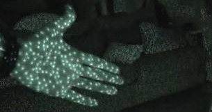
In the image above, you can see the infrared speckle. Notice at the top of the user’s hand, some of speckles are distorted. Such information might be used by the sensor to detect more than just one 3D position. It might also be used to detect shape. This is done in other computer vision algorithms that use structured light techniques.

This light is read in by an infrared camera (or sensor). It’s just like a regular camera, but for infrared light instead of visible light.

The light has patterns in it. It is randomly generated at the factory, but if you look at it, you’ll notice that it’s not uniform. Because of this, the Kinect can match the patterns of dot clusters to hard-coded images it has of the projected pattern. This hard-coded data is embedded at manufacturing.

Once this pattern is read in through the infrared camera, it looks for correlations. If it finds a good correlation, it will consider it a match. The processor within the kinect is then able to use this information to triangulate the 3D position of the points.

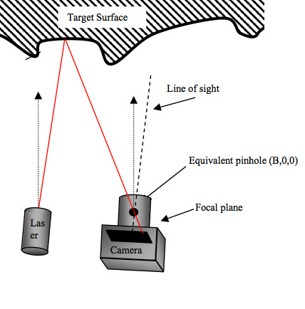
Notice that if the surface the dot hits is farther or closer, it will land on a different pixel within the camera. The pixel it lands on tells us the direction the light took through the camera's focal point. And because we know which exact dot it was that came from the projector, we know its original trajectory also. The last piece of information we need is the relative positions of the camera and projector relative to each other. This is hard coded into the kinect. This forms a triangle. Using geometry (triangulation), we can determine the 3D position of the surface. Of course, it’s not perfectly precise, but I’m told it is accurate to within an inch in height and 3 mm in width.

http://ntuzhchen.blogspot.com/2010/12/how-kinect-works-prime-sense.html

http://www.joystiq.com/2010/06/19/kinect-how-it-works-from-the-company-behind-the-tech/

According to some sources, the Kinect is also able to detect changes in the pattern due to surface roughness of the object it lands on. I'm not sure if the kinect uses this information.

After all this math, the Kinect is able to produce a depth map, like the following. The different shades/colors represent different depths.

2. Filter the raw depth data with a bilateral filter to remove erroneous measurements.

A bilateral filter performs smoothing. Basically, it goes through each pixel and recalculates the pixel’s value based on the values around it. It does this in a window around the pixel. The amount used from different pixels are weighted, so that some contribute more and some less. The pixels that are closest to the center of the filter and are similar to the center depth value receive a higher weight.

The following is an image that has had bilateral filtering applied to it.

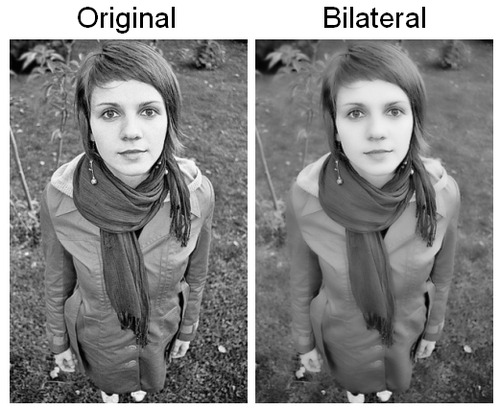
Of course, the above example gray 2D image. But, you get the point. It smooths out the differences between pixels. This has the effect of reducing some clarity, but in exchange it removes a lot of errors, which is what we need when the image is noisy.

But, now consider the following 2D image. It’s a 2D image, but it represents 3D depth values. Bilateral filtering can be applied to this depth map just like we did in the 2D gray image! The result is that the errors in the 3D depths are smoothed out.

An important feature of bilateral filters is that they preserve sharp edges because it will not smooth as much between pixels that have large differences.

Technical details of the a Kinect-fusion-like algorithm and the bilateral filter can be found here: http://gmeyer3.projects.cs.illinois.edu/cs498dwh/final/

http://en.wikipedia.org/wiki/Bilateral_filter

3. Convert the raw depth map into a map of vertices with their corresponding normal vectors.

So, now we have a filtered depth map, which is a picture that represents depth from the point of view of the infrared sensor. But, what we need to convert this 2D+gray representation into 3D coordinates with metric units, such as millimeters. To do this, we create a vertex for each point in the image where x is the x pixel, y is the y pixel, and z is the depth value. Then, we use a calibrated matrix to back-project these points (convert them) such that they are in metric units. Multiplying by matrix K will do this for us. What results is a vertex map. A vertex map is just like a depth map except that it is 3D and instead of using color to represent the depth, we use an actual z coordinate. So, it’s no longer a 2D image. It is now a point cloud.

Here are some example normal vectors and vertices. The start of the arrow represents the location of the vertice. The normal vector represents the direction pointing away from the surface.

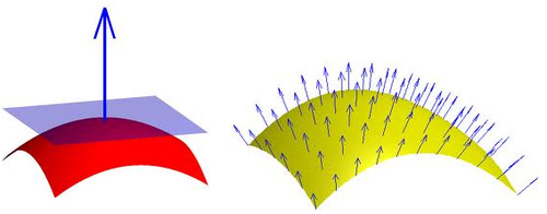
So, for each pixel in the depth map/point cloud, we calculate one of these vectors.

The following is a visualization of the normal vectors. The different colors represent different directions that the surfaces face.

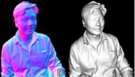
We calculate the normal for each vertice by getting the cross product between neighboring pixels. Remember, the vertices came from a depth map. So they are arranged in a regular grid just like the pixels of the depth map. So, its neighbors are the pixels that surround it. When calculating the normal, we just choose vertice that came from the x+1 pixel in the depth map and also the vertice that came from the y+1 pixel in the depth map. With these two vertices plus the center vertice, we calculate the normal for the center vertice.

We’ll find out why we need the normal and vertices in the next step, where the vertex and normal vectors are used. Note that applying bilateral filtering greatly improves the quality of the normal produced for each vertice. You might read the phrase “normal maps”. This is similar to depth map, but instead the color of each pixel represents the direction of the normal. Similar colors represent similar directions.

Also, we don’t just do this once. We actually compute a pyramid of this data! What the hell is that right? Well, it’s where you create multiple copies of the depth map at smaller (or larger) resolutions. Like this:

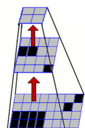
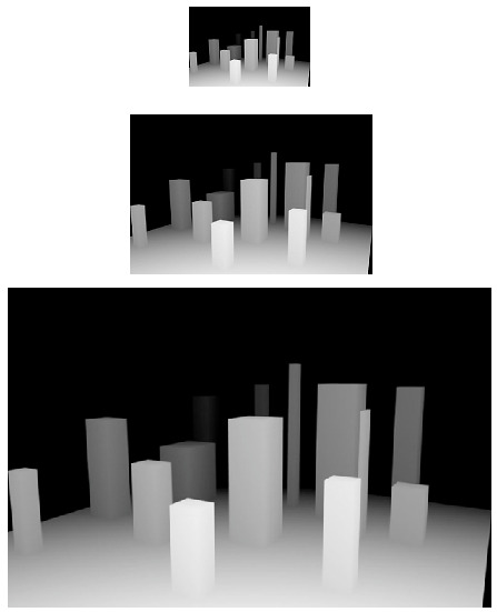
Each level in this depth-map pyramid has half the size/resolution of the previous. Kinect Fusion uses 3 levels, starting with the original depth map image at the bottom. With each level, we recalculate and store the vertices and their normals.

4. Grab a vertex map and normal map from the current model we’ve already constructed from previous iterations of the algorithm.

If we have already taken a previous depth map, then we have model already to compare our new depth map to. Our current model is simply the model we’ve constructed with all previous data. We can use the model to generate a list of vertices and normal vectors that represent it. This is just like the vertices and normal vectors from the previous step.

5. Run the ICP (Iterative Closest Point) algorithm on the two vertex and normal maps

(the new one from the camera and the one from the current model). This will generate a rotation and translation that minimizes the distance/error between the two point clouds. This 6DOF transformation (rotation and translation which has 6 degrees of freedom) tells us the cameras position relative to the current model.

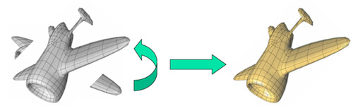
A typical Iterative Closest Point works as follows, it is trying to find the rotation and movement that will best align two point clouds like the one above. You can see that one point cloud is the whole airplane, but notice the wing pieces that are disconnected. That is a second point cloud that we want to match with the plane model.

The most important part of ICP is choosing the best starting positions of the two models so that is close to the correct match. The initial starting point is the pose of the previous frame because we assume the camera started there and has moved some small distance from there.

ICP figures out the solution by calculating how well the two models match at the current positions. But you can measure how well they match in many different ways. The typical ICP algorithm uses point-to-point errors. For every point in the first point cloud, it finds the closest point in the second point cloud and marks them as corresponding points. Then it tries to find some translation and rotation that will minimize the total error between all the corresponding point pairs. Once it finds a transformation (translation and rotation) that is sufficiently good for this iteration, it will then save those positions and repeat the algorithm.

The way that microsofts algorithm determines correspondences is not by finding the closest point in the second cloud. Instead the algorithm assumes that the changes between frames are small, because it is done in real time. So, it uses projective associations, where the two point clouds are projected into the camera’s sensor. The points that land on the same pixel are corresponding points.

It will continue doing ICP and getting closer and closer matches between the two point clouds after every iteration until they finally settle on a locally minimal match. This algorithm doesn’t always work though. You have to give it a good initial guess for how the point clouds match before it starts. Otherwise it won’t converge to a good answer. If the error is too large, then the depth map will be rejected and will not be merged with the current model.

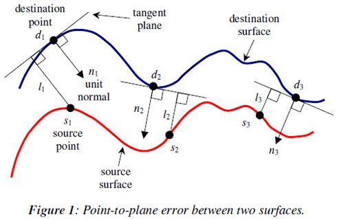
The metric used by Kinect Fusion to estimate the error between corresponding points is called the point-plane metric. Below is a diagram of this metric. Basically, instead of calculating the distance between points, it calculates the shortest distance between the line that is parallel to the surface at the first point, called the tangent line, and its corresponding point in the second cloud. This is the distance (error) used by the algorithm. For whatever reason, this converges to a good match much faster than the point-to-point metric.

Once we find a good match between the models, we now know the relative 3D position of the camera and the current model. We can also merge the current depth image with our existing model to get an even better, more refined model.

Kinect Fusion’s corresponding point pairs are not determined using the closest point method. The closest point method would find the closest point in the second cloud for each point in the first cloud and make them corresponding point pairs. Instead kinfu decides the point correspondences between models using “projective data association”. Basically it works by transforming the points from the current frame and the previous frame so that they are viewed from the same point of view. The initial guess for the pose of the current frame is the pose of the previous frame. Then, to explain it simply, it projects all of the points from both clouds into the image plane at this point of view. Then, correspondences are assigned to each point in the current depth data by selecting any of the points from the second cloud that were projected onto the same pixel in this virtual image plane. It’s sort of like overlaying the two point clouds from the same point of view and then shooting bullets through it from the viewer’s position. Wherever a bullet hits the first cloud and then the second cloud, is a correspondence.

Getting corresponding point pairs using projective data association allows ICP to run a GPU in real-time. BUT, this method assumes that motions are small between each frame! This is important. If you’re using a less powerful GPU, then it won’t function correctly. It works by taking the last frames vertices and transforming them with the same transform as the estimated current depth data. The first time ICP runs, the estimated pose of the camera is the pose we found for the last frame. This makes it so that the vertices from both depth maps are in the same coordinate system and are with respect to one view point. Then you project the last frame’s vertices into the camera to determine which virtual pixels of the current depth image land on. Because the camera has moved, some of the data may be off of the sensor’s image. In other words, the two images won’t overlap 100%. So, you ignore the ones where they don’t overlap. Wherever the vertices from the previous frame land on the new depth map, that’s where their corresponding points are. So, you can take the first one that lands on each pixel of the current depth map. Those are the corresponding points. Then you run ICP with these corresponding points. It will estimate the error, find a transform to minimize the error, and then repeat ICP again until a good match is found or it has tried too many times.

Calculating the transformation that minimizes the error between models

Upon each iteration of ICP it calculates the best transformation that minimizes the estimated error between the two models. The error is estimated by using the point-plane metric as described above. But, we haven’t talked about how to actually calculate the transformation that minimizes this error. They say: “We make a linear approximation to solve this system, by assuming only an incremental transformation occurs between frames [3, 17]. The linear system is computed and summed in parallel on the GPU using a tree reduction. The solution to this 6x6 linear system is then solved on the CPU using a Cholesky decomposition.”

Note: I think that instead of guessing that the pose of the latest frame is the same as the last frame, we might want to guess that it keeps moving in the sort of direction it was moving by tracking its motion over multiple frames and using that to predict future motion. This might improve results if motions are larger than expected by the algorithm.

Note: In the papers it refers to perspective projection of the Vi-1 vertices (vertices from the previous frame). It means to project those vertices back into the image coordinates of the sensor (a 2D image).

Merge the new depth data with the current model using the pose we just calculated.

Note that instead of using the filtered depth data, we are going to use the raw depth to add onto the current model. This is because the filter reduces noise, but it also reduces important details that we want in the final model. Any noise will be reduced as multiple iterations of the algorithm smooth out errors.

Now that we know how the new data and the existing model fit together, we can merge the data into a new, more refined and more detailed model. This is done using the Truncated Surface Distance Function (TSDF). A TSDF is calculated for the new point cloud that represents the latest depth measurements, also called the latest depth frame. We already have a TSDF for the current model. So, we combine them using weighted averaging?

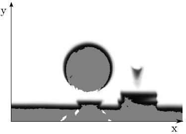
A TSDF looks something like the following when you look at just 2D section of the scene. The grey area is where no depth measurements have yet been made, and it may be because it is within a surface. The white area is where depth measurements have been made, but there was nothing there. The black is where depth measurements have been made, and it found a surface there. The TSDF assigns a value to each pixel in this grid. It finds the distance between each pixel and the closest cloud point in the current depth map we just got from the camera. This number is positive, if it’s outside of a surface, and negative if inside an area where we haven’t measured yet. We create one of these TSDFs for the new data and one for current model.

Once we have the two TSDFs, we can merge them into a single TSDF using weighted averging. This gives us our final surface representation.

We then generate the final 3D surface model by performing a ray-casting algorithm on the new TSDF.

Our new data has now been added into our current model, giving us our final model that includes all the data we have so far. Now we ready to display it to the user!

To render it, we use an algorithm called ray casting. This helps us decide what a virtual camera in that is looking at the virtual model would see. We do this by casting a ray from each pixel in the image through the focal point of the virtual camera, and do some math to figure out what is the first surface that the ray intersects with.

If the object is 100% opaque, meaning that light cannot go through it, then we know what pixel to display: it is the 3d point in the model that the ray hit. We get the value of this point and assign it to the pixel in the output image that the ray was generated from. If the pixel in the image is larger than a single 3D point, which it most likely will be, we can sample the 3D points that should be seen in the pixel and combine them into a single pixel value that represents all those 3D points from the current view point.

Color resolution is done via super resolution techniques? That way, the highest resolution texture is used. But I have not found much detail on this in the literature yet, so I’m not completely sure how it’s done.

Because we know the position of the regular color camera relative to the infrared camera, we can also perform ray casting on the color image of the scene to decide which points on the model the pixels should be assigned to. We can determine whether the image in the camera will give us the best resolution so far of the model of any given section of the model. We do this by determining 1) if we have any color data about that point yet, and 2) if we do, what angle and distance was the color resolution obtained previously? The angle and distance determines how well we can see the surface’s real colors. This will tell us whether the current camera’s perspective gives us the best resolution for a part of the model or not. If it does give us the best resolution, then we can assign the image to that section of the model. We may also want to try to guess/determine the “real” color of the point, that is invariant to lighting conditions. That way, we can then determine how the color will be scene at different viewpoints and make it look more natural when merged with nearby sections that may have used different images for color texture.

When the ray casting is performed, we can use the colors of the super resolution color model.

If the 3D model is represented with surfaces that light can pass through (opacity is less than 100%) then we can let the ray continue through the surface and pick up more color values as it goes, until the ray’s energy has been completely depleted and can travel through the surface no further. I do not believe the Kinect allows opacity of the model to be less than 100% though.

Finally the algorithm repeats in real-time around 30 times a second with every new image from the Kinect camera and sensors!

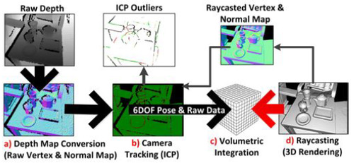
Each step of the system is run in parallel on a GPU. The different steps are: a) Depth Map Conversion to vertices and their normal. B) Camera pose (tracking) using ICP from the current depth frame to the previous depth frame. C) Given the global pose of the camera, the TSDF is merged with the current model’s TSDF. D) Ray casting to construct the current view that is displayed to the user, as well as using this ray cast to construct a vertices and their normals for this view point, which will be used in the next iteration of the algorithm in the ICP (camera pose/tracking) step.

Because Kinfu uses a TSDF, it basically constructs surfaces, rather than point clouds to display to the user. Surfaces better represents real objects and the results are more aesthetically pleasing.

As you’ve seen, the system continually tracks the 6DOF pose (6 degrees of freedom pose) of the camera and fuses live depth data from the camera into a single global 3D model in real-time. As the user explores the space, new views of the physical scene are revealed and these are fused into the same model. The reconstruction therefore grows in detail as new depth measurements are added. Holes are filled, and the model becomes more complete and refined over time.

Dictionary

AR – Augmented Reality

6DOF – 6 Degrees of Freedom the x, y and z axis plus 3 rotation axis?

Live Depth Frame – Just like the frames of a video, but in this case it is depth. The frames of a video are the individual images that make up the video.

Bundle Adjustment

Given a set of images depicting a number of 3D points from different viewpoints, bundle adjustment can be defined as the problem of simultaneously refining the 3D coordinates describing the scene geometry as well as the parameters of the relative motion and the optical characteristics of the camera(s) employed to acquire the images, according to an optimality criterion involving the corresponding image projections of all points.

Bundle adjustment is almost always used as the last step of every feature-based 3D reconstruction algorithm. It amounts to an optimization problem on the 3D structure and viewing parameters (i.e., camera pose and possibly intrinsic calibration and radial distortion), to obtain a reconstruction which is optimal under certain assumptions regarding the noise pertaining to the observed image features: If the image error is zero-mean Gaussian, then bundle adjustment is the Maximum Likelihood Estimator. Its name refers to the bundles of light rays originating from each 3D feature and converging on each camera's optical center, which are adjusted optimally with respect to both the structure and viewing parameters. Bundle adjustment was originally conceived in the field of photogrammetry during 1950s and has increasingly been used by computer vision researchers during recent years.

SLAM – Stands for Simultaneous Localization and Mapping.

(http://en.wikipedia.org/wiki/Simultaneous_localization_and_mapping)

Simultaneous localization and mapping (SLAM) is a technique used by robots and autonomous vehicles to build up a map within an unknown environment (without a priori knowledge), or to update a map within a known environment (with a priori knowledge from a given map), while at the same time keeping track of their current location.

SLAM is therefore defined as the problem of building a model leading to a new map, or repetitively improving an existing map, while at the same time localizing the robot within that map. In practice, the answers to the two characteristic questions cannot be delivered independently of each other.

ICP – Iterative Closest Point - In robotics ICP is often referred to “scan matching”.

Iterative Closest Point (ICP) is an algorithm employed to minimize the difference between two clouds of points. ICP is often used to reconstruct 2D or 3D surfaces from different scans, to localize robots and achieve optimal path planning (especially when wheel odometry is unreliable due to slippery terrain), to co-register bone models, etc.

The following is a great explanation of ICP. I also saved it locally as “ICP - Powerpoint Presentation – Very Good explanation”

http://www.cs.technion.ac.il/~cs236329/tutorials/ICP.pdf

http://en.wikipedia.org/wiki/Iterative_closest_point

Basically, on every iteration of the algorithm, the cost of points that are far away from their nearest neighbors forces the transformation to move them closer ,even if other points might move farther away from their closest matches. But, then on the next iteration, the points that had close matches will not have new closest matches and the algorithm will continue to find better and better transformations until it finds a local optimum transformation. It is only a locally optimal transformation though because it requires that the initial guess be good. If it wasn’t good, it may never find the right match.

It’s also possible to use ICP sort of algorithms for non-rigid transformations!

The point to plane metric has been shown to cause ICP to converge much faster than one that uses the point to point error metric.

Here is a really nice pdf of how the point-to-plane metric works. (saved locally as “icp - point-to-plane metric explanation.pdf”)

http://www.comp.nus.edu.sg/~lowkl/publications/lowk_point-to-plane_icp_techrep.pdf

Basically, you find the closest point between the two point clouds, just like before. But the metric or cost of their distance is calculated differently. Instead we calculate the distance between the source point and a tangent line of the destination point. The paper mentions another paper about why this converges faster than the point-to-point metric.

SDF signed distance function (SDF) introduced in [7] for the purpose of fusing partial depth scans while mitigating problems related to mesh-based reconstruction algorithms. The SDF represents surface interfaces as zeros, free space as positive values that increase with distance from the nearest surface, and (possibly) occupied space

with a similarly negative value.

Marching Cubes Algorithm –

The marching cubes algorithm is a bit confusing. What is clear is that it is used to generate the surface from a point cloud. SDF is generated from a point clouds. As mentioned before, the SDF represents surface interfaces as zeros, free space as positive values that increase with distance from the nearest surface, and (possibly) occupied space

with a similarly negative value. So, it has been shown that a good way to find the optimal surface reconstruction from this information is simply to find the weighted average of these SDF values. I assume that this averaging is done between two point clouds to get the final SDF of the combination. Then the marching cubes algorithm can be applied to this so that it finds the surface approximation that best passes through the zero point. It is approximated by checking each cube in a 3D grid. We decide whether the corners of the grids are positive or negative in the SDF. If they are negative, they are inside the surface. If they are positive, they are outside the surface. So then we split the cube in standardized ways to separate the outside corners and standard points on the cube from those that are inside the surface. Connect all of these from every cube in the 3D grid and you’ve got yourself the surface!

Here is a website that I found the most useful in understanding marching cubes. The best information is in the links at the end. http://users.polytech.unice.fr/~lingrand/MarchingCubes/accueil.html

Ray Casting - or Volume ray casting

Volume Ray Casting. Crocodile mummy provided by the Phoebe A. Hearst Museum of Anthropology, UC Berkeley. CT data was acquired by Dr. Rebecca Fahrig, Department of Radiology, Stanford University, using a Siemens SOMATOM Definition, Siemens Healthcare. The image was rendered by Fovia's High Definition Volume Rendering® engine

The technique of volume ray casting can be derived directly from the rendering equation. It provides results of very high quality, usually considered to provide the best image quality. Volume ray casting is classified as image based volume rendering technique, as the computation emanates from the output image, not the input volume data as is the case with object based techniques. In this technique, a ray is generated for each desired image pixel. Using a simple camera model, the ray starts at the center of projection of the camera (usually the eye point) and passes through the image pixel on the imaginary image plane floating in between the camera and the volume to be rendered. The ray is clipped by the boundaries of the volume in order to save time. Then the ray is sampled at regular or adaptive intervals throughout the volume. The data is interpolated at each sample point, the transfer function applied to form an RGBA sample, the sample is composited onto the accumulated RGBA of the ray, and the process repeated until the ray exits the volume. The RGBA color is converted to an RGB color and deposited in the corresponding image pixel. The process is repeated for every pixel on the screen to form the completed image.

#Kinect #Kinect Fusion #Kinfu #Computer Vision #ICP #Iterative Closest Point #Raycast #3D Models #3D MOdelling #Truncated Surface Distance Function #TSDF #SDF #Surface Distance Function

21 notes · View notes