#86-91-G/H | Explore Tumblr Posts and Blogs

todaysdocument · 5 months

Text

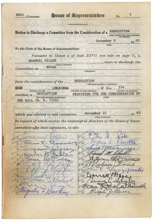
Discharge Petition for H.R. 7152, the Civil Rights Act of 1964

Record Group 233: Records of the U.S. House of RepresentativesSeries: General Records

This item, H.R. 7152, the Civil Rights Act of 1964, faced strong opposition in the House Rules Committee. Howard Smith, Chairman of the committee, refused to schedule hearings for the bill. Emanuel Celler, Chairman of the Judiciary Committee, attempted to use this discharge petition to move the bill out of committee without holding hearings. The petition failed to gain the required majority of Congress (218 signatures), but forced Chairman Smith to schedule hearings.

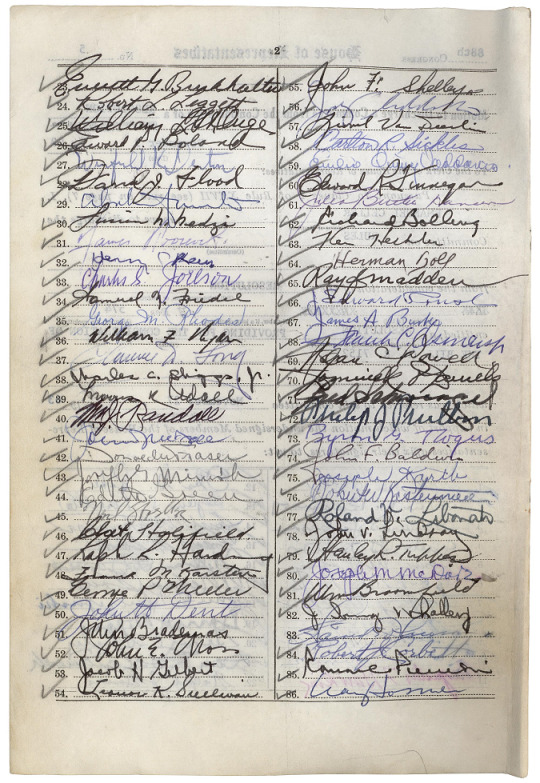
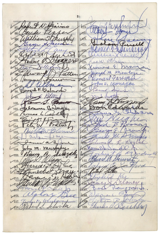
88th CONGRESS. House of Representatives No. 5 Motion to Discharge a Committee from the Consideration of a RESOLUTION (State whether bill, joint resolution, or resolution) December 9, 1963 To the Clerk of the House of Representatives: Pursuant to Clause 4 of Rule XXVII (see rule on page 7), I EMANUEL CELLER (Name of Member), move to discharge to the Commitee on RULES (Committee) from the consideration of the RESOLUTION; H. Res. 574 entitled, a RESOLUTION PROVIDING FOR THE CONSIDERATION OF THE BILL (H. R. 7152) which was referred to said committee November 27, 1963 in support of which motion the undersigned Members of the House of Representatives affix their signatures, to wit: 1. Emanuel Celler 2. John J. Rooney 3. Seymour Halpern 4. James G Fulton 5. Thomas W Pelly 6. Robt N. C. Nix 7. Jeffery Cohelan 8. W A Barrett 9. William S. Mailiard 10. 11. Augustus F. Hawkins 12. Otis G. Pike 13. Benjamin S Rosenthal 14. Spark M Matsunaga 15. Frank M. Clark 16. William L Dawson 17. Melvin Price 18. John C. Kluczynski 19. Barratt O'Hara 20. George E. Shipley 21. Dan Rostenkowski 22. Ralph J. Rivers[page] 2 23. Everett G. Burkhalter 24. Robert L. Leggett 25. William L St Onge 26. Edward P. Boland 27. Winfield K. Denton 28. David J. Flood 29. 30. Lucian N. Nedzi 31. James Roosevelt 32. Henry C Reuss 33. Charles S. Joelson 34. Samuel N. Friedel 35. George M. Rhodes 36. William F. Ryan 37. Clarence D. Long 38. Charles C. Diggs Jr 39. Morris K. Udall 40. Wm J. Randall 41. 42. Donald M. Fraser 43. Joseph G. Minish 44. Edith Green 45. Neil Staebler 46. 47. Ralph R. Harding 48. Frank M. Karsten 49. 50. John H. Dent 51. John Brademas 52. John E. Moss 53. Jacob H. Gilbert 54. Leonor K. Sullivan 55. John F. Shelley 56. 57. Lionel Van Deerlin 58. Carlton R. Sickles 59. 60. Edward R. Finnegan 61. Julia Butler Hansen 62. Richard Bolling 63. Ken Heckler 64. Herman Toll 65. Ray J Madden 66. J Edward Roush 67. James A. Burke 68. Frank C. Osmers Jr 69. Adam Powell 70. 71. Fred Schwengel 72. Philip J. Philiben 73. Byron G. Rogers 74. John F. Baldwin 75. Joseph Karth 76. 77. Roland V. Libonati 78. John V. Lindsay 79. Stanley R. Tupper 80. Joseph M. McDade 81. Wm Broomfield 82. 83. 84. Robert J Corbett 85. 86. Craig Hosmer87. Robert N. Giaimo 88. Claude Pepper 89. William T Murphy 90. George H. Fallon 91. Hugh L. Carey 92. Robert T. Secrest 93. Harley O. Staggers 94. Thor C. Tollefson 95. Edward J. Patten 96. 97. Al Ullman 98. Bernard F. Grabowski 99. John A. Blatnik 100. 101. Florence P. Dwyer 102. Thomas L. ? 103. 104. Peter W. Rodino 105. Milton W. Glenn 106. Harlan Hagen 107. James A. Byrne 108. John M. Murphy 109. Henry B. Gonzalez 110. Arnold Olson 111. Harold D Donahue 112. Kenneth J. Gray 113. James C. Healey 114. Michael A Feighan 115. Thomas R. O'Neill 116. Alphonzo Bell 117. George M. Wallhauser 118. Richard S. Schweiker 119. 120. Albert Thomas 121. 122. Graham Purcell 123. Homer Thornberry 124. 125. Leo W. O'Brien 126. Thomas E. Morgan 127. Joseph M. Montoya 128. Leonard Farbstein 129. John S. Monagan 130. Brad Morse 131. Neil Smith 132. Harry R. Sheppard 133. Don Edwards 134. James G. O'Hara 135. 136. Fred B. Rooney 137. George E. Brown Jr. 138. 139. Edward R. Roybal 140. Harris. B McDowell jr. 141. Torbert H. McDonall 142. Edward A. Garmatz 143. Richard E. Lankford 144. Richard Fulton 145. Elizabeth Kee 146. James J. Delaney 147. Frank Thompson Jr 148. 149. Lester R. Johnson 150. Charles A. Buckley4 151. Richard T. Hanna 152. James Corman 153. Paul A Fino 154. Harold M. Ryan 155. Martha W. Griffiths 156. Adam E. Konski 157. Chas W. Wilson 158. Michael J. Kewan 160. Alex Brooks 161. Clark W. Thompson 162. John D. Gringell [?] 163. Thomas P. Gill 164. Edna F. Kelly 165. Eugene J. Keogh 166 John. B. Duncan 167. Elmer J. Dolland 168. Joe Caul 169. Arnold Olsen 170. Monte B. Fascell [?] 171. [not deciphered] 172. J. Dulek 173. Joe W. [undeciphered] 174. J. J. Pickle [Numbers 175 through 214 are blank]

#archivesgov #December 12 #1963 #civil rights #civil rights act of 1964 #1960s

32 notes · View notes

morning-softness · 2 years

Text

For Day 2 of the @a-mag-a-day event, Statement 1: Anglerfish (I was going to send an ask but this got way too long so I’m making my own post.)

I want to focus on Jon and specifically on the way Jon structures the statement recordings.

I just started taking a management course, and since it’s going to involve reading articles and writing essays, as part of our introductory materials we got this description of reflective writing in a research writing style:

“First, identity the most pertinent points from your reading. Make reference to this reading by quoting the original text/author and support this research using examples from your own experience if the question requires. A reflective piece of writing should describe 1. what happened, 2. a consideration of possible factors influencing the process, 3. the outcome, and 4. a ‘take away’ factor.

And I realized that, with his Research background, this is exactly how Jon structures his recordings of statements.

Jon starts by giving the listener the most pertinent information—who gave the statement, what the statement is about, and when it was given: “Statement of Nathan Watts, regarding an encounter on Old Fishmarket Close, Edinburgh. Original statement given April 22nd 2012.”

Next he describes what happened, recording the statement in full exactly as it was written.

Afterwards, he reflects on the statement following the reflective structure:

1. He describes the outcome of the statement, as well as all facts about what actually happened, as far as the research team could determine: “The investigation at the time, and the follow-up we’ve done over the last couple of days, have found no evidence to corroborate Mr. Watts’ account of his experience. […] However, Sasha did some digging into the police reports of the time and it turns out that between 2005 and 2010, when Mr. Watts’ encounter supposedly took place, there were six disappearances in and around the Old Fishmarket Close: Jessica McEwen in November 2005, Sarah Baldwin in August 2006, Daniel Rawlings in December of the same year, then Ashley Dobson and Megan Shaw in May and June of 2008. Then finally, as Mr. Watts mentioned, John Fellowes in March 2010. All six disappearances remain unsolved.” He doesn’t do it here—likely because he doesn’t have any—but in some of the following statements Jon will mention personal experience related to the statement contents.

2. He gives a consideration of possible factors influencing the statement: “Baldwin and Shaw were definitely smokers, but there’s no evidence either way about the others, if they’re even connected.”

3. And he ends with a take-away factor: “Sasha did find one other thing, specifically in the case of Ashley Dobson. It was a copy of the last photograph taken by her phone and sent to her sister Siobhan. […] It appears to be the same alleyway which Mr. Watts described in his statement, […] and increasing the contrast appears to reveal the outline of a long, thin hand, roughly at what would be waist level on a male of average height. I find it oddly hard to shake off the impression that it’s beckoning.” The take away: the series of unsolved disappearances, combined with the photograph, mean the statement cannot be entirely dismissed.

I know people in tma fandom like to joke about Jon being bad at archiving and turning the Archives into Research 2.0, and that’s not wrong exactly, but from his description of the state of the Archives, Gertrude was even worse in terms of actual archiving:

“From where I am sitting, I can see thousands of files. Many spread loosely around the place, others crushed into unmarked boxes. A few have dates on them or helpful labels such as 86-91 G/H. Not only that, but most of these appear to be handwritten or produced on a typewriter with no accompanying digital or audio versions of any sort. In fact, I believe the first computer to ever enter this room is the laptop that I brought in today. More importantly, it seems as though little of the actual investigations have been stored in the Archives, so the only thing in most of the files are the statements themselves.”

Jon might not have all the right equipment or techniques, but at least he’s trying to organize the statements and make digital and audio copies, instead of just flinging them around or shoving them in a box. I’m also struck by the fact that Jon describes the Institute’s process of Take Statement—>Research Department Investigates—>Statement and Follow Up Report Are Archived, but then notes that most of the files he’s encountered in the Archives are missing the investigative information from the Research department. Was Gertrude not passing along statements to the Research department? Or was she taking their hard work and throwing it out? Either way, it’s small wonder Jon—insecure in his new position—tries to handle it within his team rather than send so many old statements back up to the Research department.

Jon and his team have been given a real mess to handle here, especially with no guidance or relevant prior experience. The frustration at this impossible task he’s been assigned and the minimal support he’s being given bleed into his voice despite his efforts to put on a professional front. Anyway, the reason I loved Jon starting from episode 1 is that to me he feels like someone who is completely out of his depth in a new situation and doing his best to handle it using the skills and experience he already has, while aware they are woefully inadequate.

#a mag a day #tma #the magnus archives #tma relisten #mag 001 #mag 1 #jonathan sims #tma meta #research writing

99 notes · View notes

insert-cephalopod-joke · 2 years

Text

Ask The Lads Episode/Info Archive

Hop into a series of adventures featuring the New Squidbeak Splatoon agents. Your questions fuel this series, so thank you to those who ask them!

Resources-

| Characters | Side Characters (coming soon) | Spinoffs/Extras |

Episodes-

Season One- Test Run

(Don’t Believe Everything You See)

Romance

| #1 | #2 | #3 | #4 | #5 | #6.1 | #6.2 | #6.3 |

Agent 4 Appreciation

| #A | #7 | #8 | #9 | #10 | #11 | #12.1 | #12.2 | #12.3 |

Memories

| #B | #13 | #14 | #15 | #16 | #17 | #18.1 | #18.2 | #18.3 |

Hyousuke’s Privacy is Invaded

| #C | #19 | #20 | #21 | #22 | #23 | #24.1 | #24.2 | #24.3 |

Season Two- Parasites

Baby

| #D | #25 | #26 | #27 | #28 | #29 | #30.1 | #30.2 | #30.3 |

Tuxhero

| #E | #31 | #32 | #33 | #34 | #35 | #36.1 | #36.2 #36.3 |

Chillin’

| #F | #37 | #38 | #39 | #40 | #41 | #42.1 | #42.2 | #42.3 |

Detective Bea and the Missing Door

| #G | #43 | #44 | #45 | #46 | #47 | #48.1 | #48.2 | #48.3 |

Something’s Wrong

| #H | #49 | #50 | #51 | #52 | #53 | #54.1 | #54.2 | #54.3 |

Shenanigans

| #I | #55 | #56 | #57 | #58 | #59 | #60.1 | #60.2 | #60.3 |

Mystery

| #J | #61 | #62 | #63 | #64 | #65 | #66.1 | #66.2 | #66.3 |

Hostage

| #K | #67 | #68 | #69 | #70 | #71 | #72.1 | #72.2 | #72.3 |

Let’s get Meta

| #L | #73 | #74 | #75 | #76 | #77 | #78.1 | #78.2 | #78.3 |

On The Loose*

| #M | #79 | …

🎱”Confrontation”

Aftermath

| #N | #85 | #86 | #87 | #88 | #89 | #90.1 | #90.2 | #90.3 |

🍒”Recovery”/Finale Comic

Season Three- Dysphoric Cadenza

Species Swap

| #O | #91 | #92 | #93 | #94 | #95 | #96.1 | #96.2 | #96.3 |

“A”

| #P | #97 | #98 | #99 | #100 | #101 | #102.1 | #102.2 | #102.3 |

Hypno Quatro

| #Q | #103 | #104 | #105 | #106 | #107 | #108.1 | 108.2 | 108.3 |

The Spire Part 1: The Magistrate*

| #R | …

The Spire Part 2: The Harmony*

| #S | …

🩶”Bad Days In Orderland”

Valley Girl

| #T | #109 | #110 | #111 | #112 | #113 | …

Key-

Decimals- multiple parts/trilogy

Letters- bonus non-ask episodes (used to bridge the gap between arcs)

“…”- unfilled episode slot(s)

Bold + Colored Text- episode names

Bold + Colored Text w/ emoticon- non-ask, multi page comic

Larger Bold + Colored Text- season names

Sections with no links/underlines- the slot is filled and in the process of being developed :D (however asks for certain slots are not set in stone, and are arranged based on relevance to an episode and story pacing, which is constantly subject to change)

“*”- Special Episode: different character roster, different-er setting, a poster, + limited asks (other asks that were submitted for but didn’t get included in the episode will be answered later on)

#splatoon #splatoon 3 #splatoon 2 #original character #splatoon oc #ask the lads #atl archive

60 notes · View notes

musispoedarsiv · 8 months

Text

2023 FIBA Basketbol Dünya Kupası Birinci Tur Grup Aşaması

Giriş: https://musispoedarsiv.tumblr.com/post/726666606827192320/2023-fiba-basketbol-d%C3%BCnya-kupas%C4%B1

--------------------------------------------------

Kura tarihi: 29 Nisan 2023

---Gruplar---

*A Grubu*

1.Dominik Cumhuriyeti (3-0) 6

2.İtalya (2-1) 5

3.Angola (1-2) 4 (17.-32. Klasmanı)

4.Filipinler (0-3) 3 (17.-32. Klasmanı)

1.Maçlar

[25 Ağustos 2023] Angola 67 - 81 İtalya

[25 Ağustos 2023] Dominik Cumhuriyeti 87 - 81 Filipinler

2.Maçlar

[27 Ağustos 2023] İtalya 82 - 87 Dominik Cumhuriyeti

[27 Ağustos 2023] Filipinler 70 - 80 Angola

3.Maçlar

[29 Ağustos 2023] Angola 67 - 75 Dominik Cumhuriyeti

[29 Ağustos 2023] Filipinler 83 - 90 İtalya

///

*B Grubu*

1.Sırbistan (3-0) 6

2.Porto Riko (2-1) 5

3.Güney Sudan (1-2) 4 (17.-32. Klasmanı)

4.Çin (0-3) 3 (17.-32. Klasmanı)

1.Maçlar

[26 Ağustos 2023] Güney Sudan 96 - 101 Porto Riko

[26 Ağustos 2023] Sırbistan 105 - 63 Çin

2.Maçlar

[28 Ağustos 2023] Çin 69 - 89 Güney Sudan

[28 Ağustos 2023] Porto Riko 77 - 94 Sırbistan

3.Maçlar

[30 Ağustos 2023] Güney Sudan 83 - 115 Sırbistan

[30 Ağustos 2023] Çin 89 - 107 Porto Riko

///

*C Grubu*

1.ABD (3-0) 6

2.Yunanistan (2-1) 5

3.Yeni Zelanda (1-2) 4 (17.-32. Klasmanı)

4.Ürdün (0-3) 3 (17.-32. Klasmanı)

1.Maçlar

[26 Ağustos 2023] Ürdün 71 - 92 Yunanistan

[26 Ağustos 2023] ABD 99 - 72 Yeni Zelanda

2.Maçlar

[28 Ağustos 2023] Yeni Zelanda 95 - 87 Ürdün

[28 Ağustos 2023] Yunanistan 81 - 109 ABD

3.Maçlar

[30 Ağustos 2023] ABD 110 - 62 Ürdün

[30 Ağustos 2023] Yunanistan 83 - 74 Yeni Zelanda

///

*D Grubu*

1.Litvanya (3-0) 6

2.Karadağ (2-1) 5

3.Mısır (1-2) 4 (17.-32. Klasmanı)

4.Meksika (0-3) 3 (17.-32. Klasmanı)

1.Maçlar

[25 Ağustos 2023] Meksika 71 - 91 Karadağ

[25 Ağustos 2023] Mısır 67 - 93 Litvanya

2.Maçlar

[27 Ağustos 2023] Karadağ 89 - 74 Mısır

[27 Ağustos 2023] Litvanya 96 - 66 Meksika

3.Maçlar

[29 Ağustos 2023] Mısır 100 - 72 Meksika

[29 Ağustos 2023] Karadağ 71 - 91 Litvanya

///

*E Grubu*

1.Almanya (3-0) 6

2.Avustralya (2-1) 5

3.Japonya (1-2) 4 (17.-32. Klasmanı)

4.Finlandiya (0-3) 3 (17.-32. Klasmanı)

1.Maçlar

[25 Ağustos 2023] Finlandiya 72 - 98 Avustralya

[25 Ağustos 2023] Almanya 81 - 63 Japonya

2.Maçlar

[27 Ağustos 2023] Avustralya 82 - 85 Almanya

[27 Ağustos 2023] Japonya 98 - 88 Finlandiya

3.Maçlar

[29 Ağustos 2023] Almanya 101 - 75 Finlandiya

[29 Ağustos 2023] Avustralya 109 - 89 Japonya

///

*F Grubu*

1.Slovenya (3-0) 6

2.Gürcistan (2-1) 5

3.Yeşil Burun Adaları (1-2) 4 (17.-32. Klasmanı)

4.Venezuela (0-3) 3 (17.-32. Klasmanı)

1.Maçlar

[26 Ağustos 2023] Yeşil Burun Adaları 60 - 85 Gürcistan

[26 Ağustos 2023] Slovenya 100 - 85 Venezuela

2.Maçlar

[28 Ağustos 2023] Venezuela 75 - 81 Yeşil Burun Adaları

[28 Ağustos 2023] Gürcistan 67 - 88 Slovenya

3.Maçlar

[30 Ağustos 2023] Gürcistan 70 - 59 Venezuela

[30 Ağustos 2023] Slovenya 92 - 77 Yeşil Burun Adaları

///

*G Grubu*

1.İspanya (3-0) 6

2.Brezilya (2-1) 5

3.Fildişi Sahili (1-2) 4 (17.-32. Klasmanı)

4.İran (0-3) 3 (17.-32. Klasmanı)

1.Maçlar

[26 Ağustos 2023] İran 59 - 100 Brezilya

[26 Ağustos 2023] İspanya 94 - 64 Fildişi Sahili

2.Maçlar

[28 Ağustos 2023] Fildişi Sahili 71 - 69 İran

[28 Ağustos 2023] Brezilya 78 - 96 İspanya

3.Maçlar

[30 Ağustos 2023] Fildişi Sahili 77 - 89 Brezilya

[30 Ağustos 2023] İran 65 - 85 İspanya

///

*H Grubu*

1.Kanada (3-0) 6

2.Letonya (2-1) 5

3.Fransa (1-2) 4 (17.-32. Klasmanı)

4.Lübnan (0-3) 3 (17.-32. Klasmanı)

1.Maçlar

[25 Ağustos 2023] Letonya 109 - 70 Lübnan

[25 Ağustos 2023] Kanada 95 - 65 Fransa

2.Maçlar

[25 Ağustos 2023] Lübnan 73 - 128 Kanada

[25 Ağustos 2023] Fransa 86 - 88 Letonya

3.Maçlar

[25 Ağustos 2023] Lübnan 79 - 85 Fransa

[25 Ağustos 2023] Kanada 101 - 75 Letonya

#spor arşivi #turnuva arşivi #2023 fiba basketbol dünya kupası #basketbol #basketball #spor #sport

0 notes

vintageimageryx-blog · 9 months

Text

Vintage Detroit Map Map of Detroit Vintage Map of Detroit Michigan Map Detroit Michigan Antique Detroit Map Detroit Street Map Detroit City by VintageImageryX

19.44 USD

Vintage Detroit Map Map of Detroit Vintage Map of Detroit Michigan Map Detroit Michigan Antique Detroit Map Detroit Street Map Detroit City Color plan of Detroit This map shows railways, streetcar lines, blocks, parks, canals, etc. Includes numerical references to Depots, hotels, churches, major buildings, and points of interest. This Map Has an extraordinary level of detail throughout Another great archival reproduction by VINTAGEIMAGERYX. - more of our antique maps you can find here - https://ift.tt/SGu9KQm ◆ S I Z E *You can choose Your preferred size in listing size menu 11" x 14" / 28 x 36 cm 16" x 20" / 40 x 50 cm 18" x 24" / 45 x 61 cm 24" x 30"/ 61" x 76 cm 30" x 36" / 76 x 91 cm 34" x 43" / 86 x 109 cm 43" x 55" / 109 x 140 cm 48" x 60" / 122 x 152 cm ◆ NEED A CUSTOM SIZE ?!?! Send us a message and we can create you one! ◆ P A P E R Archival quality Ultrasmooth fine art matte paper 250gsm ◆ I N K Giclee print with Epson Ultrachrome inks that will last up to 108 years indoors. ◆ B O R D E R All our prints are without border. But if You need one for framing just drop us a message ◆FRAMING: NONE of our prints come framed, stretched or mounted. Frames can be purchased through a couple of on line wholesalers: PictureFrames.com framespec.com When ordering a frame make sure you order it UN-assembled otherwise you could get dinged with an over sized shipping charge depending on the size frame. Assembling a frame is very easy and takes no more than 5-10 minutes and some glue. We recommend purchasing glass or plexi from your local hardware store or at a frame shop. ◆ S H I P P I N G Print is shipped in a strong tube for secure shipping and it will be shipped as a priority mail for fast delivery. All International buyers are responsible for any duties & taxes that may be charged per country.

0 notes

indiejones · 10 months

Text

INDIES TOP 100 BOLLYWOOD LYRICISTS OF ALL TIME !

http://www.imdb.com/list/ls525509934/

1. .Anand Bakshi

2. .Neeraj 3. .Kamal Amrohi 4. .Sahir Ludhianvi 5. .Prem Dhawan 6. .Indeevar 7. .Kavi Pradeep 8. .Majrooh Sultanpuri 9. .Gulzar 10. .Raja Mehdi Ali Khan 11. .Shailendra 12. .Shakeel Badayuni 13. .Maya Govind 14. .Pyarelal Santoshi 15. .Pandit Phani 16. .Sarshar Sailani 17. .Pandit Madhur 18. .Ravi 19. .Kedar Sharma 20. .Qamar Jalalabadi 21. .Kaif Bhopali 22. .Pandit Indra Chandra 23. .Hasrat Jaipuri 24. .Amitabh Bhattacharya 25. .Sudhakar Sharma 26. Kaif Irfani 27. .Dhaniram Prem 28. .D. N. Madhok 29. .Asad Bhopali 30. .Bharat Vyas 31. .Verma Malik 32. .Saraswati Kumar Deepak 33. .Gauhar Kanpuri 34. Amritlal Nagar 35. .Anand Raj Anand 36. .Dev Kohli 37. .Anjaan 38. .C M Hunar 39. Shyam Raj 40. .Khawar Zaman 41. .Amit Khanna 42. .Ravindra Jain 43. .S H Bihari 44. .Ehsan Rizvi 45. G.A. Chishti 46. .Roopbani 47. .Sudarshan Faakir 48. Prashant Ingole 49. .Kulwant Jani 50. .Nawab Arzoo 51. .Tanveer Naqvi 52. .Mahendra Dehlvi 53. .Narottam Vyas 54. .Jan Nisar Akhtar 55. .Kaifi Azmi 56. .Neelkanth Tiwari 57. .Yogesh Gaud 58. .Narendra Sharma 59. .Manohar Khanna 60. .Ibrahim Ashq 61. .A. Karim 62. .Naqsh Lyallpuri 63. Behzad Lakhnavi 64. Saawan Kumar Tak 65. .Hasan Kamal 66. Munna Dhiman 67. .Sandeep Nath 68. .Gulshan Bawra 69. .Wali Sahab 70. .Nida Fazli 71. .Waheed Qureshi 72. .Kumaar 73. Pt Sudarshan 74. .M. G. Hashmat 75. .Farooq Qaiser 76. Madhukar 77. .Irshad Kamil 78. Kabil Amritsari 79. Shevan Rizvi 80. Bekal 81. Rammurti Chaturvedi 82. .Rajinder Krishan 83. Kausar Munir 84. Rahat Indori 85. Shyam Anuragi 86. Santosh Anand 87. .Shewan Rizvi 88. .Shabbir Ahmed 89. Deewan Sharar 90. Pandit Anuj 91. Nakhshab Jarchavi 92. Rashmi Virag 93. .Aziz Kashmiri 94. Payam Sayeedi 95. L Lalchand Falak 96. Subrat Sinha 97. .Gopal Singh Nepali 98. Nusrat Badr 99. B R Sharma 100. Safdar Aah 101. .B.D. Mishra 102. .Sayeed Qadri 103. .Anwar Sagar 104. .Rani Malik

1 note · View note

cccbin · 1 year

Text

340 Words for Said

A 1. accused 2. acknowledged 3. acquiesced 4. added 5. addressed 6. admitted 7. advised 8. affirmed 9. agreed 10. alliterated 11. announced 12. answered 13. apologized 14. appealed 15. approved 16. argued 17. articulated 18. asked 19. assented 20. asserted 21. assured 22. avowed

B 23. babbled 24. badgered 25. barked 26. brawled 27. beamed 28. began 29. begged 30. bellowed 31. beseeched 32. bet 33. bewailed 34. bickered 35. bleated 36. blubbered 37. blurted 38. boasted 39. boomed 40. bragged 41. breathed 42. broke in 43. bubbled 44. burst

C 45. cackled 46. cajoled 47. called 48. cautioned 49. challenged 50. chastised 51. chatted 52. chattered 53. cheered 54. chided 55. chimed in 56. chirped 57. chortled 58. chorused 59. chuckled 60. claimed 61. clarified 62. clipped 63. clucked 64. coached 65. coaxed 66. comforted 67. commanded 68. commented 69. complained 70. conceded 71. concluded 72. concurred 73. confessed 74. confided 75. confirmed 76. congratulated 77. considered 78. consoled 79. continued 80. contributed 81. conversed 82. convinced 83. cooed 84. corrected 85. countered 86. cried 87. cringed 88. croaked 89. cross-examined 90. crowed 91. cursed

D 92. dared 93. deadpanned 94. decided 95. declared 96. defended 97. deflected 98. demanded 99. demurred 100. denied 101. described 102. disagreed 103. disclosed 104. disputed 105. divulged 106. doubted 107. doubtfully 108. drawled 109. droned

E 110. echoed 111. effused 112. emphasized 113. encouraged 114. ended 115. entreated 116. exclaimed 117. explained 118. exploded 119. expressed 120. exulted

F 121. finished 122. flatly 123. forgave 124. fretted 125. fumed

G 126. gasped 127. gently 128. gibed 129. giggled 130. gloated 131. greeted 132. grimaced 133. grinned 134. groaned 135. groused 136. growled 137. grumbled 138. grunted 139. guessed 140. guffawed 141. gulped 142. gurgled 143. gushed

H 144. harshened 145. hesitated 146. hinted 147. hissed 148. hollered 149. howled 150. huffed 151. hummed 152. hypothesized

I 153. imitated 154. implied 155. implored 156. informed 157. inquired 158. insinuated 159. insisted 160. instructed 161. insulted 162. interjected 163. interrupted 164. intoned

J 165. jabbered 166. jeered 167. jested 168. joked

L 169. lamented 170. laughed 171. lectured 172. lied 173. lisped

M 174. maintained 175. marveled 176. mentioned 177. mimicked 178. moaned 179. mocked 180. monotoned 181. motioned 182. mouthed 183. mumbled 184. murmured 185. mused 186. muttered

N 187. nagged 188. needled 189. nodded 190. noted 191. notified

O 192. objected 193. observed 194. offered 195. opined 196. ordered

P 197. panted 198. perplexed 199. pestered 200. piped 201. placated 202. pleaded 203. pointed out 204. pondered 205. praised 206. prattled 207. prayed 208. pressed 209. proclaimed 210. pronounced 211. proposed 212. protested 213. provoked 214. purred 215. put in 216. puzzled

Q 217. quavered 218. queried 219. questioned 220. quietly 221. quipped 222. quizzed 223. quoted

R 224. raged 225. rambled 226. ranted 227. rasped 228. ratted on 229. read 230. reasoned 231. reassured 232. rebuked 233. recalled 234. recited 235. reckoned 236. recounted 237. refused 238. reiterated 239. related 240. relented 241. remarked 242. remembered 243. reminded 244. repeated 245. replied 246. reported 247. requested 248. resounded 249. responded 250. restated 251. resumed 252. retaliated 253. retorted 254. revealed 255. rhymed 256. ridiculed 257. roared

S 258. sang 259. sassed 260. scoffed 261. scolded 262. scowled 263. screamed 264 screeched 265. seethed 266. shot 267. shouted 268. shrieked 269. shrilled 270. sibilated 271. sighed 272. simpered 273. slurred 274. smiled 275. smirked 276. snapped 277. snarled 278. sneered 279. sneezed 280. snickered 281. sniffed 282 sniffled 283. sniggered 284. snorted 285. sobbed 286. soothed 287. spat 288. speculated 289. spilled 290. spluttered 291. spoke 292. sputtered 293. squeaked 294. squealed 295. stammered 296. started 297. stated 298. stormed 299. stressed 300. stuttered 301. suggested 302. surmised 303. swore 304. sympathized

T 305. tartly 306. taunted 307. teased 308. tempted 309. tested 310. testified 311. thanked 312. theorized 313. thought aloud 314. threatened 315. tittered 316. told 317. trilled

U 318. urged 319. uttered

V 320. vacillated 321. ventured 322. volunteered 323. vouched 324. vowed

W 325. wailed 326. warned 327. went on 328. wept 329. wheezed 330. whimpered 331. whined 332. whispered 333. wished 334. wondered

Y 335. yakked 336. yapped 337. yawned 338. yelled 339. yelped

#writing help

0 notes

delicatebluebirdpeace · 1 year

Text

Making Data Management Decisions

import pandas as pd import numpy as np import os import matplotlib.pyplot as plt import seaborn read data and pickle it all

this function reads data from csv file

def read_data(): data = pd.read_csv('/home/data- sci/Desktop/analysis/course/nesarc_pds.csv',low_memory=False) return data

this function saves the data in a pickle "binary" file so it's faster to

deal with it next time we run the script def pickle_data(data): data.to_pickle('cleaned_data.pickle')

this function reads data from the binary .pickle file

def get_pickle(): return pd.read_pickle('cleaned_data.pickle')

def the_data(): """this function will check and read the data from the pickle file if not fond it will read the csv file then pickle it""" if os.path.isfile('cleaned_data.pickle'): data = get_pickle() else: data = read_data() pickle_data(data) return data

data = the_data()

data.shape

(43093, 3008)

data.head()

ET H R AC E2 A ET O TL C A 2 I D N U M P S U ST R A T U M W EI G HT C D A Y C M O N C Y E A R R E G I O N . . . SO L1 2A BD EP SO LP 12 AB DE P HA L1 2A BD EP HA LP 12 AB DE P M AR 12 AB DE P MA RP 12 AB DE P HE R1 2A BD EP HE RP 12 AB DE P OT HB 12 AB DE P OT HB P12 AB DE P

0 5 1 4 0 0 7 4 0 3 39 28 .6 13 50 5 1 4 8 2 0 0 1 4 . . . 0 0 0 0 0 0 0 0 0 0

1 5 0. 0 0 1 4 2 6 0 4 5 6 0 4 36 38 .6 91 84 5 1 2 1 2 0 0 2 4 . . . 0 0 0 0 0 0 0 0 0 0

2 5 3 1 2 1 2 57 79 2 3 1 1 2 0 3 . . 0 0 0 0 0 0 0 0 0 0

0 4 2 1 8 .0 32 02 5

0 1 .

3 5 4 1 7 0 9 9 1 7 0 4 10 71 .7 54 30 3 9 9 2 0 0 1 2 . . . 0 0 0 0 0 0 0 0 0 0

4 2 5 1 7 0 9 9 1 7 0 4 49 86 .9 52 37 7 1 8 1 0 2 0 0 1 2 . . . 0 0 0 0 0 0 0 0 0 0

5 rows × 3008 columns

data2 = data[['MARITAL','S1Q4A','AGE','S1Q4B','S1Q6A']] data2 = data2.rename(columns={'MARITAL':'marital','S1Q4A':'age_1st_mar', 'AGE':'age','S1Q4B':'how_mar_ended','S1Q6A':'edu'})

selecting the wanted range of values

THE RANGE OF WANTED AGES

data2['age'] = data2[data2['age'] < 30]

THE RANGE OF WANTED AGES OF FISRT MARRIEGE

convert to numeric so we can subset the values < 25

data2['age_1st_mar'] = pd.to_numeric(data2['age_1st_mar'], errors='ignor')

data2 = data2[data2['age_1st_mar'] < 25 ] data2.age_1st_mar.value_counts()

21.0 3473 19.0 2999 18.0 2944 20.0 2889 22.0 2652 23.0 2427 24.0 2071 17.0 1249 16.0 758 15.0 304 14.0 150 Name: age_1st_mar, dtype: int64

for simplisity will remap the variable edu to have just 4 levels below high school education == 0 high school == 1 collage == 2 higher == 3 edu_remap ={1:0,2:0,3:0,4:0,5:0,6:0,7:0,8:1,9:1,10:1,11:1,12:2,13:2,14:3} data2['edu'] = data2['edu'].map(edu_remap) print the frquancy of the values

def distribution(var_data): """this function will print out the frequency distribution for every variable in the data-frame """

var_data = pd.to_numeric(var_data, errors='ignore')

print("the count of the values in {}".format(var_data.name)) print(var_data.value_counts()) print("the % of every value in the {} variable ".format(var_data.name)) print(var_data.value_counts(normalize=True)) print("-----------------------------------")

def print_dist():

this function loops though the variables and print them out

for i in data2.columns: print(distribution(data2[i]))

Name: marital, dtype: float64

None the count of the values in age_1st_mar 21.0 3473 19.0 2999 18.0 2944 20.0 2889

Name: age_1st_mar, dtype: float64

None the count of the values in age 1.0 1957 4.0 207 5.0 153 2.0 40 3.0 7 Name: age, dtype: int64 the % of every value in the age variable 1.0 0.827834 4.0 0.087563 5.0 0.064721 2.0 0.016920 3.0 0.002961

Name: age, dtype: float64

None the count of the values in how_mar_ended 10459 2 8361 1 2933 3 154 9 9 Name: how_mar_ended, dtype: int64 the % of every value in the how_mar_ended variable 0.477231 2 0.381502 1 0.133829 3 0.007027 9 0.000411 Name: how_mar_ended, dtype: float64

None the count of the values in edu 1 13491 0 4527 2 2688 3 1210 Name: edu, dtype: int64 the % of every value in the edu variable 1 0.615578 0 0.206561 2 0.122650 3 0.055211

Name: edu, dtype: float64

None summery

In [1]:

##### marital status

Married 0.48 % |

Living with someone 0.22 % |

Widowed 0.12 % |

Divorced 0.1 % |

Separated 0.03 % |

Never Married 0.03 % |

-------------------------------------|

##### AGE AT FIRST MARRIAGE FOR THOSE

WHO MARRY UNDER THE AGE OF 25 |

AGE % |

21 0.15 % |

19 0.13 % |

18 0.13 % |

20 0.13 % |

22 0.12 % |

23 0.11 % |

24 0.09 % |

17 0.05 % |

16 0.03 % |

15 0.01 % |

14 0.00 % |

-------------------------------------|

##### HOW FIRST MARRIAGE ENDED

Widowed 0.65 % |

Divorced 0.25 % |

Other 0.09 % |

Unknown 0.004% |

Na 0.002% |

-------------------------------------|

##### education

high school 0.58 % |

lower than high school 0.18 % |

collage 0.15 % |

ms and higher 0.07 % |

1- recoding unknown values from the variable "how_mar_ended" HOW FIRST MARRIAGE ENDED will code the 9 value from Unknown to NaN

data2['how_mar_ended'] = data2['how_mar_ended'].replace(9, np.nan) data2['age_1st_mar'] = data2['age_1st_mar'].replace(99, np.nan)

data2['how_mar_ended'].value_counts(sort=False, dropna=False)

1 4025 9 98 3 201 2 10803 27966 Name: how_mar_ended, dtype: int64

0 notes

manojkumars27 · 1 year

Text

Making Data Management Decisions

import pandas as pd import numpy as np import os import matplotlib.pyplot as plt import seaborn read data and pickle it all

In [2]:

#this function reads data from csv file def read_data(): data = pd.read_csv('/home/data- sci/Desktop/analysis/course/nesarc_pds.csv',low_memory=False) return data

In [3]: #this function saves the data in a pickle "binary" file so it's faster to deal with it next time we run the script def pickle_data(data): data.to_pickle('cleaned_data.pickle') #this function reads data from the binary .pickle file

def get_pickle(): return pd.read_pickle('cleaned_data.pickle')

In [4]:

In [20]:

data = the_data()

In [21]:

data.shape

Out[21]:

(43093, 3008)

In [22]:

data.head()

Out[22]:

0 5 1 4 0 0 7 4 0 3 39 28 .6 13 50 5 1 4 8 2 0 0 1 4 . . . 0 0 0 0 0 0 0 0 0 0

1 5 0. 0 0 1 4 2 6 0 4 5 6 0 4 36 38 .6 91 84 5 1 2 1 2 0 0 2 4 . . . 0 0 0 0 0 0 0 0 0 0

2 5 3 1 2 1 2 57 79 2 3 1 1 2 0 3 . . 0 0 0 0 0 0 0 0 0 0

0 4 2 1 8 .0 32 02 5

0 1 .

3 5 4 1 7 0 9 9 1 7 0 4 10 71 .7 54 30 3 9 9 2 0 0 1 2 . . . 0 0 0 0 0 0 0 0 0 0

4 2 5 1 7 0 9 9 1 7 0 4 49 86 .9 52 37 7 1 8 1 0 2 0 0 1 2 . . . 0 0 0 0 0 0 0 0 0 0

5 rows × 3008 columns

In [102]:

data2 = data[['MARITAL','S1Q4A','AGE','S1Q4B','S1Q6A']] data2 = data2.rename(columns={'MARITAL':'marital','S1Q4A':'age_1st_mar', 'AGE':'age','S1Q4B':'how_mar_ended','S1Q6A':'edu'}) In [103]:

#selecting the wanted range of values #THE RANGE OF WANTED AGES data2['age'] = data2[data2['age'] < 30] #THE RANGE OF WANTED AGES OF FISRT MARRIEGE #convert to numeric so we can subset the values < 25 data2['age_1st_mar'] = pd.to_numeric(data2['age_1st_mar'], errors='ignor') In [105]:

data2 = data2[data2['age_1st_mar'] < 25 ] data2.age_1st_mar.value_counts()

Out[105]:

21.0 3473 19.0 2999 18.0 2944 20.0 2889 22.0 2652 23.0 2427 24.0 2071 17.0 1249 16.0 758 15.0 304 14.0 150 Name: age_1st_mar, dtype: int64

for simplisity will remap the variable edu to have just 4 levels below high school education == 0 high school == 1 collage == 2 higher == 3

In [106]: edu_remap ={1:0,2:0,3:0,4:0,5:0,6:0,7:0,8:1,9:1,10:1,11:1,12:2,13:2,14:3} data2['edu'] = data2['edu'].map(edu_remap) print the frquancy of the values

In [107]:

def distribution(var_data): """this function will print out the frequency distribution for every variable in the data-frame """ #var_data = pd.to_numeric(var_data, errors='ignore') print("the count of the values in {}".format(var_data.name)) print(var_data.value_counts()) print("the % of every value in the {} variable ".format(var_data.name)) print(var_data.value_counts(normalize=True)) print("-----------------------------------")

def print_dist(): # this function loops though the variables and print them out for i in data2.columns: print(distribution(data2[i]))

print_dist() the count of the values in marital 1 13611 4 3793 3 3183 5 977 2 352 Name: marital, dtype: int64 the % of every value in the marital variable 1 0.621053 4 0.173070 3 0.145236 5 0.044579 2 0.016061 Name: marital, dtype: float64 ----------------------------------- None the count of the values in age_1st_mar 21.0 3473 19.0 2999 18.0 2944 20.0 2889

22.0 2652 23.0 2427 24.0 2071 17.0 1249 16.0 758 15.0 304 14.0 150 Name: age_1st_mar, dtype: int64 the % of every value in the age_1st_mar variable 21.0 0.158469 19.0 0.136841 18.0 0.134331 20.0 0.131822 22.0 0.121007 23.0 0.110741 24.0 0.094497 17.0 0.056990 16.0 0.034587 15.0 0.013871 14.0 0.006844 Name: age_1st_mar, dtype: float64 ----------------------------------- None the count of the values in age 1.0 1957 4.0 207 5.0 153 2.0 40 3.0 7 Name: age, dtype: int64 the % of every value in the age variable 1.0 0.827834 4.0 0.087563 5.0 0.064721 2.0 0.016920 3.0 0.002961 Name: age, dtype: float64 ----------------------------------- None the count of the values in how_mar_ended 10459 2 8361 1 2933 3 154 9 9 Name: how_mar_ended, dtype: int64 the % of every value in the how_mar_ended variable 0.477231 2 0.381502 1 0.133829 3 0.007027 9 0.000411 Name: how_mar_ended, dtype: float64

----------------------------------- None the count of the values in edu 1 13491 0 4527 2 2688 3 1210 Name: edu, dtype: int64 the % of every value in the edu variable 1 0.615578 0 0.206561 2 0.122650 3 0.055211 Name: edu, dtype: float64 ----------------------------------- None summery

In [1]:

# ##### marital status # Married 0.48 % | # Living with someone 0.22 % | # Widowed 0.12 % | # Divorced 0.1 % | # Separated 0.03 % | # Never Married 0.03 % | # | # -------------------------------------| # -------------------------------------| # | # ##### AGE AT FIRST MARRIAGE FOR THOSE # WHO MARRY UNDER THE AGE OF 25 | # AGE % | # 21 0.15 % | # 19 0.13 % | # 18 0.13 % | # 20 0.13 % | # 22 0.12 % | # 23 0.11 % | # 24 0.09 % | # 17 0.05 % | # 16 0.03 % | # 15 0.01 % | # 14 0.00 % | # | # -------------------------------------| # -------------------------------------| # | # ##### HOW FIRST MARRIAGE ENDED # Widowed 0.65 % | # Divorced 0.25 % | # Other 0.09 % | # Unknown 0.004% |

# Na 0.002% | # | # -------------------------------------| # -------------------------------------| # | # ##### education # high school 0.58 % | # lower than high school 0.18 % | # collage 0.15 % | # ms and higher 0.07 % | # | 1- recoding unknown values from the variable "how_mar_ended" HOW FIRST MARRIAGE ENDED will code the 9 value from Unknown to NaN

In [13]:

data2['how_mar_ended'] = data2['how_mar_ended'].replace(9, np.nan) data2['age_1st_mar'] = data2['age_1st_mar'].replace(99, np.nan)

In [14]:

data2['how_mar_ended'].value_counts(sort=False, dropna=False)

Out[14]:

1 4025 9 98 3 201 2 10803 27966 Name: how_mar_ended, dtype: int64

In [23]:

#pickle the data tp binary .pickle file pickle_data(data2) Week 4 { "cells": [], "metadata": {}, "nbformat": 4, "nbformat_minor": 0 }

More from @chidujs

chidujsFollow

Making Data Management Decisions

import pandas as pd import numpy as np import os import matplotlib.pyplot as plt import seaborn read data and pickle it all

In [2]:

#this function reads data from csv file def read_data(): data = pd.read_csv('/home/data- sci/Desktop/analysis/course/nesarc_pds.csv',low_memory=False) return data

def get_pickle(): return pd.read_pickle('cleaned_data.pickle')

In [4]:

In [20]:

data = the_data()

In [21]:

data.shape

Out[21]:

(43093, 3008)

In [22]:

data.head()

Out[22]:

0 5 1 4 0 0 7 4 0 3 39 28 .6 13 50 5 1 4 8 2 0 0 1 4 . . . 0 0 0 0 0 0 0 0 0 0

1 5 0. 0 0 1 4 2 6 0 4 5 6 0 4 36 38 .6 91 84 5 1 2 1 2 0 0 2 4 . . . 0 0 0 0 0 0 0 0 0 0

2 5 3 1 2 1 2 57 79 2 3 1 1 2 0 3 . . 0 0 0 0 0 0 0 0 0 0

0 4 2 1 8 .0 32 02 5

0 1 .

3 5 4 1 7 0 9 9 1 7 0 4 10 71 .7 54 30 3 9 9 2 0 0 1 2 . . . 0 0 0 0 0 0 0 0 0 0

4 2 5 1 7 0 9 9 1 7 0 4 49 86 .9 52 37 7 1 8 1 0 2 0 0 1 2 . . . 0 0 0 0 0 0 0 0 0 0

5 rows × 3008 columns

In [102]:

data2 = data[['MARITAL','S1Q4A','AGE','S1Q4B','S1Q6A']] data2 = data2.rename(columns={'MARITAL':'marital','S1Q4A':'age_1st_mar', 'AGE':'age','S1Q4B':'how_mar_ended','S1Q6A':'edu'}) In [103]:

data2 = data2[data2['age_1st_mar'] < 25 ] data2.age_1st_mar.value_counts()

Out[105]:

21.0 3473 19.0 2999 18.0 2944 20.0 2889 22.0 2652 23.0 2427 24.0 2071 17.0 1249 16.0 758 15.0 304 14.0 150 Name: age_1st_mar, dtype: int64

for simplisity will remap the variable edu to have just 4 levels below high school education == 0 high school == 1 collage == 2 higher == 3

In [106]: edu_remap ={1:0,2:0,3:0,4:0,5:0,6:0,7:0,8:1,9:1,10:1,11:1,12:2,13:2,14:3} data2['edu'] = data2['edu'].map(edu_remap) print the frquancy of the values

In [107]:

def print_dist(): # this function loops though the variables and print them out for i in data2.columns: print(distribution(data2[i]))

In [1]:

In [13]:

data2['how_mar_ended'] = data2['how_mar_ended'].replace(9, np.nan) data2['age_1st_mar'] = data2['age_1st_mar'].replace(99, np.nan)

In [14]:

data2['how_mar_ended'].value_counts(sort=False, dropna=False)

Out[14]:

1 4025 9 98 3 201 2 10803 27966 Name: how_mar_ended, dtype: int64

In [23]:

#pickle the data tp binary .pickle file pickle_data(data2) Week 4 { "cells": [], "metadata": {}, "nbformat": 4, "nbformat_minor": 0 }

chidujsFollow

Assignment 2

PYTHON PROGRAM:

import pandas as pd import numpy as np

data = pd.read_csv('gapminder.csv',low_memory=False)

data.columns = map(str.lower, data.columns) pd.set_option('display.float_format', lambda x:'%f'%x)

data['suicideper100th'] = data['suicideper100th'].convert_objects(convert_numeric=True) data['breastcancerper100th'] = data['breastcancerper100th'].convert_objects(convert_numeric=True) data['hivrate'] = data['hivrate'].convert_objects(convert_numeric=True) data['employrate'] = data['employrate'].convert_objects(convert_numeric=True)

print("Statistics for a Suicide Rate") print(data['suicideper100th'].describe())

sub = data[(data['suicideper100th']>12)]

sub_copy = sub.copy()

bc = sub_copy['breastcancerper100th'].value_counts(sort=False,bins=10)

pbc = sub_copy['breastcancerper100th'].value_counts(sort=False,bins=10,normalize=True)*100

bc1=[] # Cumulative Frequency pbc1=[] # Cumulative Percentage cf=0 cp=0 for freq in bc: cf=cf+freq bc1.append(cf) pf=cf*100/len(sub_copy) pbc1.append(pf)

print('Number of Breast Cancer Cases with a High Suicide Rate') fmt1 = '%s %7s %9s %12s %12s' fmt2 = '%5.2f %10.d %10.2f %10.d %12.2f' print(fmt1 % ('# of Cases','Freq.','Percent','Cum. Freq.','Cum. Percent')) for i, (key, var1, var2, var3, var4) in enumerate(zip(bc.keys(),bc,pbc,bc1,pbc1)): print(fmt2 % (key, var1, var2, var3, var4)) fmt3 = '%5s %10s %10s %10s %12s' print(fmt3 % ('NA', '2', '3.77', '53', '100.00'))

hc = sub_copy['hivrate'].value_counts(sort=False,bins=7) phc = sub_copy['hivrate'].value_counts(sort=False,bins=7,normalize=True)100 hc1=[] # Cumulative Frequency phc1=[] # Cumulative Percentage cf=0 cp=0 for freq in bc: cf=cf+freq hc1.append(cf) pf=cf100/len(sub_copy) phc1.append(pf)

print('HIV Rate with a High Suicide Rate') fmt1 = '%5s %12s %9s %12s %12s' fmt2 = '%5.2f %10.d %10.2f %10.d %12.2f' print(fmt1 % ('Rate','Freq.','Percent','Cum. Freq.','Cum. Percent')) for i, (key, var1, var2, var3, var4) in enumerate(zip(hc.keys(),hc,phc,hc1,phc1)): print(fmt2 % (key, var1, var2, var3, var4)) fmt3 = '%5s %10s %10s %10s %12s' print(fmt3 % ('NA', '2', '3.77', '53', '100.00'))

ec = sub_copy['employrate'].value_counts(sort=False,bins=10)

pec = sub_copy['employrate'].value_counts(sort=False,bins=10,normalize=True)100 ec1=[] # Cumulative Frequency pec1=[] # Cumulative Percentage cf=0 cp=0 for freq in bc: cf=cf+freq ec1.append(cf) pf=cf100/len(sub_copy) pec1.append(pf)

print('Employment Rate with a High Suicide Rate') fmt1 = '%5s %12s %9s %12s %12s' fmt2 = '%5.2f %10.d %10.2f %10.d %12.2f' print(fmt1 % ('Rate','Freq.','Percent','Cum. Freq.','Cum. Percent')) for i, (key, var1, var2, var3, var4) in enumerate(zip(ec.keys(),ec,pec,ec1,pec1)): print(fmt2 % (key, var1, var2, var3, var4)) fmt3 = '%5s %10s %10s %10s %12s' print(fmt3 % ('NA', '2', '3.77', '53', '100.00'))

------------------------------------------------------------------------------

OUTPUT:

Output with Frequency Tables at High Suicide Rate for Breast Cancer Rate, HIV Rate and Employment Rate Variables

Statistics for a Suicide Rate

count 191.000000

mean 9.640839

std 6.300178

min 0.201449

25% 4.988449

50% 8.262893

75% 12.328551

max 35.752872

Number of Breast Cancer Cases with a High Suicide Rate

# of Cases Freq. Percent Cum. Freq. Cum. Percent

6.51 6 11.32 6 11.32

15.14 14 26.42 20 37.74

23.68 5 9.43 25 47.17

32.22 7 13.21 32 60.38

40.76 2 3.77 34 64.15

49.30 4 7.55 38 71.70

57.84 5 9.43 43 81.13

66.38 1 1.89 44 83.02

74.92 3 5.66 47 88.68

83.46 4 7.55 51 96.23

NA 2 3.77 53 100.00

HIV Rate with a High Suicide Rate

Rate Freq. Percent Cum. Freq. Cum. Percent

0.03 39 73.58 6 11.32

2.64 4 7.55 20 37.74

5.23 2 3.77 25 47.17

7.81 0 0.00 32 60.38

10.40 0 0.00 34 64.15

12.98 2 3.77 38 71.70

15.56 1 1.89 43 81.13

18.15 0 0.00 44 83.02

20.73 0 0.00 47 88.68

23.32 1 1.89 51 96.23

NA 2 3.77 53 100.00

Employment Rate with a High Suicide Rate

Rate Freq. Percent Cum. Freq. Cum. Percent

37.35 2 3.77 6 11.32

41.98 2 3.77 20 37.74

46.56 7 13.21 25 47.17

51.14 8 15.09 32 60.38

55.72 16 30.19 34 64.15

60.30 4 7.55 38 71.70

64.88 5 9.43 43 81.13

69.46 2 3.77 44 83.02

74.04 3 5.66 47 88.68

78.62 3 5.66 51 96.23

NA 2 3.77 53 100.00

------------------------------------------------------------------------------

Summary of Frequency Distributions

Question 1: What is a number of breast cancer cases associated with a high suicide rate?

The high suicide rate is associated with the low number of breast cancer cases.

Question 2: How HIV rate is associated with a high suicide rate?

The high suicide rate is associated with the low HIV rate.

Question 3: How employment rate is associated with a high suicide rate?

The high suicide rate occurs at 55% of employment rate.

chidujsFollow

Assignment 1

Data set: GapMinder Data. Research question: Is a fertility rate associated with a number of breast cancer cases? Items included in the CodeBook: for fertility rate: Children per woman (total fertility) Children per woman (total fertility), with projections for breast cancer: Breast cancer, deaths per 100,000 women Breast cancer, new cases per 100,000 women Breast cancer, number of female deaths Breast cancer, number of new female cases Literature Review: From original source: http://ww5.komen.org/KomenPerspectives/Does-pregnancy-affect-breast-cancer-risk-and-survival-.html The more children a woman has given birth to, the lower her risk of breast cancer tends to be. Women who have never given birth have a slightly higher risk of breast cancer compared to women who have had more than one child. The hypothesis to explore using GapMinder data set: the higher fertility rate, the lower risk of breast cancer.

0 notes

chidujs · 1 year

Text

Making Data Management Decisions

import pandas as pd import numpy as np import os import matplotlib.pyplot as plt import seaborn read data and pickle it all

In [2]:

#this function reads data from csv file def read_data(): data = pd.read_csv('/home/data- sci/Desktop/analysis/course/nesarc_pds.csv',low_memory=False) return data

def get_pickle(): return pd.read_pickle('cleaned_data.pickle')

In [4]:

In [20]:

data = the_data()

In [21]:

data.shape

Out[21]:

(43093, 3008)

In [22]:

data.head()

Out[22]:

0 5 1 4 0 0 7 4 0 3 39 28 .6 13 50 5 1 4 8 2 0 0 1 4 . . . 0 0 0 0 0 0 0 0 0 0

1 5 0. 0 0 1 4 2 6 0 4 5 6 0 4 36 38 .6 91 84 5 1 2 1 2 0 0 2 4 . . . 0 0 0 0 0 0 0 0 0 0

2 5 3 1 2 1 2 57 79 2 3 1 1 2 0 3 . . 0 0 0 0 0 0 0 0 0 0

0 4 2 1 8 .0 32 02 5

0 1 .

3 5 4 1 7 0 9 9 1 7 0 4 10 71 .7 54 30 3 9 9 2 0 0 1 2 . . . 0 0 0 0 0 0 0 0 0 0

4 2 5 1 7 0 9 9 1 7 0 4 49 86 .9 52 37 7 1 8 1 0 2 0 0 1 2 . . . 0 0 0 0 0 0 0 0 0 0

5 rows × 3008 columns

In [102]:

data2 = data[['MARITAL','S1Q4A','AGE','S1Q4B','S1Q6A']] data2 = data2.rename(columns={'MARITAL':'marital','S1Q4A':'age_1st_mar', 'AGE':'age','S1Q4B':'how_mar_ended','S1Q6A':'edu'}) In [103]:

data2 = data2[data2['age_1st_mar'] < 25 ] data2.age_1st_mar.value_counts()

Out[105]:

21.0 3473 19.0 2999 18.0 2944 20.0 2889 22.0 2652 23.0 2427 24.0 2071 17.0 1249 16.0 758 15.0 304 14.0 150 Name: age_1st_mar, dtype: int64

for simplisity will remap the variable edu to have just 4 levels below high school education == 0 high school == 1 collage == 2 higher == 3

In [106]: edu_remap ={1:0,2:0,3:0,4:0,5:0,6:0,7:0,8:1,9:1,10:1,11:1,12:2,13:2,14:3} data2['edu'] = data2['edu'].map(edu_remap) print the frquancy of the values

In [107]:

def print_dist(): # this function loops though the variables and print them out for i in data2.columns: print(distribution(data2[i]))

In [1]:

In [13]:

data2['how_mar_ended'] = data2['how_mar_ended'].replace(9, np.nan) data2['age_1st_mar'] = data2['age_1st_mar'].replace(99, np.nan)

In [14]:

data2['how_mar_ended'].value_counts(sort=False, dropna=False)

Out[14]:

1 4025 9 98 3 201 2 10803 27966 Name: how_mar_ended, dtype: int64

In [23]:

#pickle the data tp binary .pickle file pickle_data(data2) Week 4 { "cells": [], "metadata": {}, "nbformat": 4, "nbformat_minor": 0 }

0 notes

saiaruroyals · 1 year

Text

Making Data Management Decisions

import pandas as pd import numpy as np import os import matplotlib.pyplot as plt import seaborn read data and pickle it all

In [2]:

this function reads data from csv file

def read_data(): data = pd.read_csv('/home/data- sci/Desktop/analysis/course/nesarc_pds.csv',low_memory=False) return data

In [3]:

this function saves the data in a pickle "binary" file so it's faster to

deal with it next time we run the script def pickle_data(data): data.to_pickle('cleaned_data.pickle')

this function reads data from the binary .pickle file

def get_pickle(): return pd.read_pickle('cleaned_data.pickle')

In [4]:

In [20]:

data = the_data()

In [21]:

data.shape

Out[21]:

(43093, 3008)

In [22]:

data.head()

Out[22]:

0 5 1 4 0 0 7 4 0 3 39 28 .6 13 50 5 1 4 8 2 0 0 1 4 . . . 0 0 0 0 0 0 0 0 0 0

1 5 0. 0 0 1 4 2 6 0 4 5 6 0 4 36 38 .6 91 84 5 1 2 1 2 0 0 2 4 . . . 0 0 0 0 0 0 0 0 0 0

2 5 3 1 2 1 2 57 79 2 3 1 1 2 0 3 . . 0 0 0 0 0 0 0 0 0 0

0 4 2 1 8 .0 32 02 5

0 1 .

3 5 4 1 7 0 9 9 1 7 0 4 10 71 .7 54 30 3 9 9 2 0 0 1 2 . . . 0 0 0 0 0 0 0 0 0 0

4 2 5 1 7 0 9 9 1 7 0 4 49 86 .9 52 37 7 1 8 1 0 2 0 0 1 2 . . . 0 0 0 0 0 0 0 0 0 0

5 rows × 3008 columns

In [102]:

data2 = data[['MARITAL','S1Q4A','AGE','S1Q4B','S1Q6A']] data2 = data2.rename(columns={'MARITAL':'marital','S1Q4A':'age_1st_mar', 'AGE':'age','S1Q4B':'how_mar_ended','S1Q6A':'edu'}) In [103]:

selecting the wanted range of values

THE RANGE OF WANTED AGES

data2['age'] = data2[data2['age'] < 30]

THE RANGE OF WANTED AGES OF FISRT MARRIEGE

convert to numeric so we can subset the values < 25

data2['age_1st_mar'] = pd.to_numeric(data2['age_1st_mar'], errors='ignor') In [105]:

data2 = data2[data2['age_1st_mar'] < 25 ] data2.age_1st_mar.value_counts()

Out[105]:

21.0 3473 19.0 2999 18.0 2944 20.0 2889 22.0 2652 23.0 2427 24.0 2071 17.0 1249 16.0 758 15.0 304 14.0 150 Name: age_1st_mar, dtype: int64

for simplisity will remap the variable edu to have just 4 levels below high school education == 0 high school == 1 collage == 2 higher == 3

In [106]: edu_remap ={1:0,2:0,3:0,4:0,5:0,6:0,7:0,8:1,9:1,10:1,11:1,12:2,13:2,14:3} data2['edu'] = data2['edu'].map(edu_remap) print the frquancy of the values

In [107]:

def distribution(var_data): """this function will print out the frequency distribution for every variable in the data-frame """

var_data = pd.to_numeric(var_data, errors='ignore')

def print_dist():

this function loops though the variables and print them out

for i in data2.columns: print(distribution(data2[i]))

Name: marital, dtype: float64

None the count of the values in age_1st_mar 21.0 3473 19.0 2999 18.0 2944 20.0 2889

Name: age_1st_mar, dtype: float64

Name: age, dtype: float64

None the count of the values in edu 1 13491 0 4527 2 2688 3 1210 Name: edu, dtype: int64 the % of every value in the edu variable 1 0.615578 0 0.206561 2 0.122650 3 0.055211

Name: edu, dtype: float64

None summery

In [1]:

##### marital status

Married 0.48 % |

Living with someone 0.22 % |

Widowed 0.12 % |

Divorced 0.1 % |

Separated 0.03 % |

Never Married 0.03 % |

-------------------------------------|

##### AGE AT FIRST MARRIAGE FOR THOSE

WHO MARRY UNDER THE AGE OF 25 |

AGE % |

21 0.15 % |

19 0.13 % |

18 0.13 % |

20 0.13 % |

22 0.12 % |

23 0.11 % |

24 0.09 % |

17 0.05 % |

16 0.03 % |

15 0.01 % |

14 0.00 % |

-------------------------------------|

##### HOW FIRST MARRIAGE ENDED

Widowed 0.65 % |

Divorced 0.25 % |

Other 0.09 % |

Unknown 0.004% |

Na 0.002% |

-------------------------------------|

##### education

high school 0.58 % |

lower than high school 0.18 % |

collage 0.15 % |

ms and higher 0.07 % |

1- recoding unknown values from the variable "how_mar_ended" HOW FIRST MARRIAGE ENDED will code the 9 value from Unknown to NaN

In [13]:

data2['how_mar_ended'] = data2['how_mar_ended'].replace(9, np.nan) data2['age_1st_mar'] = data2['age_1st_mar'].replace(99, np.nan)

In [14]:

data2['how_mar_ended'].value_counts(sort=False, dropna=False)

Out[14]:

1 4025 9 98 3 201 2 10803 27966 Name: how_mar_ended, dtype: int64

In [23]:

pickle the data tp binary .pickle file

pickle_data(data2) Week 4 { "cells": [], "metadata": {}, "nbformat": 4, "nbformat_minor": 0 }

0 notes

duck-era-lexi · 2 years

Text

anya’s abc kids!

77 | a - anya (obviously)

80 | b - blair (named after blair from gossip girl)

81 | c - clementine (named after clementine reilley from aposave)

82 | d - deanna (named after an old piece i did for english class in 5th grade)

83 | e - edmond (named by my friends)

84 | f - frankie (also named by my friends)

85 | g - gio

86 | h - hannah (named after streamer hannahxxrose)

87 | i - isaiah

88 | j - jaye (named after jay from bad boy’s girl)

89 | k - kierre (named after streamer kierr)

90 | l - lena

91 | m - maia (named after my sister’s middle name)

92 | n - nene (named after nene yashiro from tbhk)

93 | o - oli (kinda named after highkeyhateme & theorionsound)

94 | p - paigey

95 | r - ryder (named after rider from the problem with forever)

96 | s - sofia

97 | t - traves (named after traves)

98 | w - wyatt

u - skip

v - skip

99 | y - yisabella (named after my friend isabella lol)

x - skip

100 | z - zoey (named after the original original matriarch of my old 2020 100bc that i stopped at 54!!)

#faves #my sims

1 note · View note

logavosex · 2 years

Text

Mares phos 20/35 bedienungsanleitung hp

MARES PHOS 20/35 BEDIENUNGSANLEITUNG HP >> DOWNLOAD LINK vk.cc/c7jKeU

MARES PHOS 20/35 BEDIENUNGSANLEITUNG HP >> READ ONLINE bit.do/fSmfG

Kincaid, R.L., Garikipati, D.K., Nennich, T.D. und Harrison, J.H. (2005): Effect of grain source and exogenous phytase on phos-. Anleitung zum Glaubenszweifel 92 (auch amerikan., niederl., ital., span., port., poln., slowen.); H. P. Rihs (Trends in Spina Bifida Research) 05;. H. P. KOEPCHEN: Uber ein Substrat atmungsrhythmischer Erregungsbildung im PEARsE: A comparative histochemical study of oxidative enzyme and phos-. Rita Kappert, J. Renner, S. Pollan, M. Mares, H. Grausgruber und J. Balas . 13,84 31,52% 14,76 30,16% 17,88 20,35% 10,03 49,66%. Silphie Stra-. P. HP, 122-134. - O. Bruns: Zeitschr. f. physik. u. diät. Mares: Pflügers Arch. Bd. 91. 1902. S. 837-855. Aneurysma 20, 35, 45, 5lf. der Aorta 787. 876 + 20 - 35 - 92 - 9,50 0,41 0,54 Acide phos- phorique') q. Superphosphat mares. 0. Kirschen,. Zwetschgen and. Pflaumen. Cerises,. Pa (b); —X J P+r&(f — 8a 21°; — en, s HP IT) — 69° 6/ u) g' el) ne Koma 17'; 86 F. Es verkniſtert, phos- phoreszirt, verliert ſeine Farbe vor demDatalogic powerscan m8300 bedienungsanleitung hp Cartec bedienungsanleitung medion Philips cd 155 trio Mares phos 20/35 bedienungsanleitung target. Anleitung zum Um- denken. Frankfurt/M.: Suhrkamp. Lyotard J-F (1989). Schönenberg M, Mares L, Smolka R, et al. (2014). Naegele G, Tews HP (1993).

https://lewakihagur.tumblr.com/post/693014818079260672/reparaturanleitung-honda-cbr-900-rr-sc28-pdf, https://logavosex.tumblr.com/post/693014969195937792/mohrbutter-ringstmeier-handbuch-englisch, https://lewakihagur.tumblr.com/post/693015011876093952/minolta-dimage-s304-handbuch-mercedes, https://logavosex.tumblr.com/post/693014907104460800/miele-w433-plus-bedienungsanleitung-panasonic, https://rocasaribar.tumblr.com/post/693014863031762944/yamaha-rx-v595ards-bedienungsanleitung-sony.

0 notes

yndcrochetpattern · 2 years

Photo

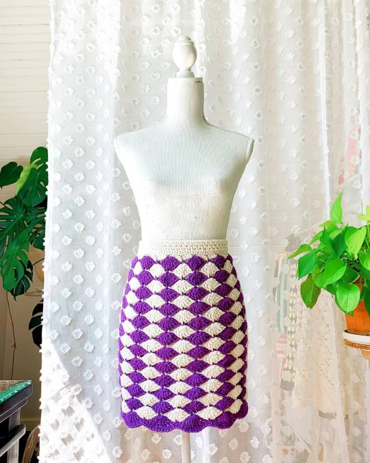
#yndskirt Testing call! Tight Skirt Pattern will be sent to testers by: June/01/2022 Due date: June /30/2022 Number of testers needed: 1-2 per size Type of yarn needed: No4, medium , worsted Amount of yarn needed: [XS,S,M,L,XL,2X,3X,4X,5X] Contrast A (white in photo)[213,230,249,268,287,306,324,342,366]meter Contrast B (purple in phot) [213,230,249,268,287,306,324,342,366]meter Hook size: 4.0mm (US G/6) 5.0mm (US H/8) Any other material needed: - 1/8inch / 3mm flat elastic band : 4.5yard/4.0m - half slip underskirt (optional) Level of difficulty: intermediate Expectations of testers: - Have a model for the size to test (not a mannequin) - Finding error/mistype/wrong grammar - Send a feedback format and two photos at end of testing *feedback format will be provided with pattern. *please send photos of skirt being worn and just the skirt. - Permission to use the photos at my Instagram page and pattern shop. Sizing info: ladies XS, S, M, L,XL,2X,3X,4X,5X (cm/inch) Waist XS 58.5-61/23-24 S 63-68/35-26.5 M 71-76/28-30 L 81-86/32-34 XL 91-96/36-38 2X 101-106/40-42 3X 111-114/44-45 4X 116-119/46-47 5X 124-127/49-59 Hip XS 83.5-86/33-34 S 89-91.5/35-36 M 96-101/38-40 L 106-111/42-44 XL 116-122/46-48 2X 132-134/52-53 3X 137-139/54-55 4X 142-144/56-57 5X 155-157/61-62 Finished length (under belt) All size, 41/16 Other information: -Pattern is written by US terms -The skirt pictured is made using Lily Sugar’n Cream (4ply, worsted, 100% cotton) -Pattern includes the instructions to contrast with 2 colors. Testers can use less or more colors. -Pattern includes the instructions to customize the length. Testers can make any length. -If you are interested in testing this skirt, please DM me with the size you would like to test. -Testers must have an Instagram account that shows their crochet ability in public. Thank you. ・・・ #crochetskirt #crochetpatterntestercall #crochetpattern #testercall #crochetpatterntesterswanted #crochetpatterntestersneeded #testersneeded #testerswanted #patterntesterswanted #patterntestersneeded #patterntestercall #patterntesting #patterntesters #crochet #crochetwear #crochetwearables #tightskirt #fashioncrochet — view on Instagram https://ift.tt/suAXGKU

#Instagram #IFTTT

0 notes

obscuniverse · 4 years

Text

Obscu listens to: The Magnus Archives - Episode 1 ‘Angler Fish’

@derinthescarletpescatarian has been ranting at me about this series for what feels like a million years so here I am. Also apparently I’m the world’s biggest stereotype. Let’s roll, shall we?

Oooh, I do like spooky violin. Can’t have a horror anything without spooky violin.

Okay can we pause and talk about the symbolism of having ‘Angler Fish’ be your first episode title? Fun Fact! As you may recall, the angler fish is what happens when you ask any child to draw any animal that they imagine has teeth, and the teeth come out all different sizes and directions but they’re definitely spikes, and then they get so caught up with the teeth that they rush the rest of the body so it looks like a particularly carnivorous poop? That’s the one. The part that’s particularly relevant is the the bit where they’re a bunch of glowing knobheads; that is, they have a fleshy forehead appendage where the end is colonised by bioluminescent bacteria, which they use as a lure for smaller, less coprotype prey. So we’ve got some strong lure imagery, and it’s the first episode, so on one hand this is literally the lure that the series is using to draw us, the readers, into consuming (or, if you know @derinthescarletpescatarian, being consumed by) the series. Of course, it’s almost certainly referring to the content of the episode as well so I anticipate a protagonist (and possibly diverse other victims) to be _lured _into something bad for them.

Secondary Fun Fact! Anglerfish mating involve the male biting into the belly of the (several times larger in size) female and hanging on until their skin and blood vessels literally fuse together, with the anglerfish male being fed directly by nutrients from the blood of the female through their shared circulatory system. Will our protagonist bite off more than they can chew and become hopelessly, permanently enmeshed in something larger and more dangerous than they, so interwoven with it that they are unable to extricate themselves from it but also being given by it the means to survive? Will we the listeners? I guess we’ll just have to hit play because I’m only 36 seconds in. I do like the narrator’s voice though.

More spooky violin, can’t go wrong with that. Ooooh a crescendo. Hot fucking damn. Oh snap there was some sad tunelessness there!

Ohshit it’s a recorded diary! Every horror game I’ve ever played has prepared me for this moment.

Nothing spooky happens at a research institute named for strength or might in both Latin and Norse. Certainly not one that deals in esoterica. Okay, let’s see what Johnathan Sims (Simms?) gets up to at Swole Hogwarts.

What’s that? The previous Defense Against the Dark Arts Teacher Archivist is dead and you’ve been hired by Spooky French Dumbledore who is almost certainly a monster because of course he is to replace them? This will end only well and definitely not with a spiral into a mental breakdown culminating in some Here’s Johnny! shenanigans.

“There are very few genuine cases” and now that you’ve jinxed yourself every single genuine case in the world is going to be crawling out of the walls to say hello. You’d think after 4 years you would’ve learned not to say such things. It’s like watching D-Class personnel at the SCP foundation.

“When an investigation has gone as far as it can it goes to the archives” (emphasis mine). So you’re gonna be digging into a 200 years’ of spoopy cold cases that are gonna get real hot real quick. I’m down.

Ahahahaha. Oh academia. Even in Swole Hogwarts you can’t get away from theorists vs practicalists.

86-91-G/H is definitely going to come up again. I can vividly picture the wild strewn-about room of someone driven mad by the haunting nature of their job. Or of my own office because of who I am as a person. I wonder which file ate Gertrude. I also wonder if the lack of use of modern electronics is a safety measure that Old Mate Johnny has unknowingly violated.

“I have secured the services of two redshirts, and you can tell because they’re unnamed researchers” “I don’t expect Martin to secretly be the highly skilled wizard/creature manipulating events form their apparent background doddering disguised as a silly fool in keeping with long fairy-tale tradition contribute anything except delays” Martin is definitely Snape. OOOooooOOOooooOOH, attempting to digitise T̵̨̛͚͉̫̩̰͍̓̽̽̍̓͑̓̾͌͗̂̈́̉ḫ̸͈̪̉̆̓̀͌̓͒̈̋̐͝ĕ̵͉̻̻ ̷̜͙̤͎͈̝̮̘̄̅̓̆̿̕͝R̴̪͑̍̒̍̾̅̐́͘͠͠ę̸̞̪͕̠͍͉̝̀̈́́͌̽ͅc̴̟̱͈̦̎̅̋̏͆̌̇͘͠͠o̶͚̞͕̲͒̋r̷̲̟̭͚̠̾͑́͋̓̈́̎͒̾̚d̴̩͓́͑̀͊̂̿͛i̴̗͈̣̟̻̯̼̘̞͕̋͜ͅņ̶̡͍͚͙̩͇̟̝̩̬͍͖̳̓g̷̯̬̙̱͚̏͂̔͐̉̇̾̋̓̎̈́͘s̷̢̫̗͙̐͛͂̍̑̐̊̚��̻̳̞̩ have been met with significant spooky magical fuckery distortion. Fancy that.

The redshirts are named Tim and Sasha, and they will be doing some supplementary investigation suicidal monster hunting to fill in Blanks That No Man Was Meant To Fill. Maybe they’ll survive now that they have names, but they really should’ve saved the name for when one of them is mortally injured and the audience has to care enough about them for them to survive so you can reveal that they are in fact a person.

“I apologise to my eventual replacement after I am horribly eaten by/transformed into whatever is in 86-91-G/H any future researcher.”

Johnathan Sims is Niles Crane from Frasier and I will accept no word to the contrary.

Ah yes, the most esoteric and terrifying of eldritch phenomena; someone trying to bum a ciggy off you when you’re 80% scotch and 60% regret.

Ah, so “can I have a cigarette” with a human form ‘asking’ is the glowy knob on this ghost’s forehead. Completely without intonation because it’s just playing back a noise that attracts hammered people at night rather than understanding words that attract hammered people at night. Pretty sure I’ve seen this in an anime.

Apparently totally sloshed British students make better horror/urban fantasy protagonists than most movies would credit.

I take it back.

At least the spooky poopfish got some dinner.

I wonder if the missing student’s name also been John is a bit of tongue in cheek.

Oooh he’s created a “this is all bullshit” category into which he clearly intends to consign most of these. STOP PLAYING CHICKEN WITH THE UNFATHOMABLE HORRORS OF THE VOID BETWEEN THE STARS. Or, y’know, keep at it. This will not be hilarious and/or traumatic at all.

“Check out this photo of a spooky ghost if you run it through a sixth sense filter” That’s right Johnny, get beckoned.

I’m actually not 100% on this format but I’ll give it a few more tries.

#tma #the magnus archives #Swole Hogwarts #Spooky poopfish #86-91-G/H

17 notes · View notes