#Agef 21

[dijonbeaune]

Le Chemin Gourmand de Nuits-Saint-Georges 2022 fait le plein

Le Chemin Gourmand de Nuits-Saint-Georges 2022 fait le plein

La 10e balade gourmande de Nuits-Saint-Georges affiche complet trois mois avant l’événement du 26 juin 2022. Son papa Pierre Mostacci est naturellement ravi. Au taquet ! Le Chemin Gourmand de Nuits-Saint-Georges 2022 accueillera 1800 participants. © D.R. Au bout du fil, Pierre Mostacci a le sourire. Il en serait presque gêné au moment d’annoncer que le Chemin Gourmand de Nuits-Saint-Georges…

[my-naomi-blog]

Week 4

INPUT 

import pandas import numpy import seaborn import matplotlib.pyplot as plt # any additional libraries would be imported here

mydata = pandas.read_csv('prostate_1.csv', low_memory=False)

# subset variables in new data frame, sub1 sub1=mydata[['AgeF','PSA', 'Cancer Volume']]

a = sub1.head print(a)

#new PSA variable, categorical 1 through 2 def PSA (row):   if row['PSA'] < 4 :      return 1   if row['PSA'] > 4 :      return 2 sub1['PSA'] = sub1.apply (lambda row: PSA (row),axis=1)

a = sub1.head print(a)

#new Age variable, categorical 1 through 2 def Age (row):   if row['AgeF']== '41-50':      return 1   if row['AgeF'] == '51-60' :      return 2   if row['AgeF'] == '61-70' :      return 3   if row['AgeF'] == '71-80' :      return 4 sub1['Age'] = sub1.apply (lambda row: Age (row),axis=1)

a = sub1.head print(a)

#new Cancer_Volume variable, categorical 1 through 4 def Cancer_Volume(row):   if row['Cancer Volume'] < 11:      return 1   if row['Cancer Volume'] >11 and row['Cancer Volume'] < 21 :      return 2   if row['Cancer Volume'] >21 and row['Cancer Volume'] <31 :      return 3   if row['Cancer Volume'] >31:      return 4 sub1['Cancer_Volume'] = sub1.apply (lambda row: Cancer_Volume(row),axis=1)

a = sub1.head print(a)

#univariate bar graph for categorical variables for PSA level # First hange format from numeric to categorical sub1["PSA"] = sub1["PSA"].astype('category')

seaborn.countplot(x="PSA", data=sub1) plt.xlabel('PSA level') plt.title('PSA level Among Adult men who visited the university medical center in the Prostate cancer Study')

#univariate bar graph for categorical variables for Age groups # First hange format from numeric to categorical sub1["AgeF"] = sub1["AgeF"].astype('category')

seaborn.countplot(x="AgeF", data=sub1) plt.xlabel('AgeF') plt.title('Age groups Among Adult men who visited the university medical center in the Prostate cancer Study')

#univariate bar graph for categorical variables for Cancer Volume # First hange format from numeric to categorical sub1["Cancer_Volume"] = sub1["Cancer_Volume"].astype('category')

seaborn.countplot(x="Cancer_Volume", data=sub1) plt.xlabel('Cancer_Volume') plt.title('Cancer Volume Among Adult men who visited the university medical center in the Prostate cancer Study')

# standard deviation and other descriptive statistics for quantitative variables

print ('PSA level') desc2 = sub1['PSA'].describe() print (desc2)

c1= sub1.groupby('PSA').size() print (c1)

print ('mode PSA level') mode1 = sub1['PSA'].mode() print (mode1)

c1= sub1.groupby('PSA').size() print (c1)

p1 = sub1.groupby('PSA').size() * 100 / len(mydata) print (p1)

# standard deviation and other descriptive statistics for quantitative variables

print ('Age') desc2 = sub1['AgeF'].describe() print (desc2)

c2= sub1.groupby('AgeF').size() print (c2)

print ('mode of Age') mode1 = sub1['AgeF'].mode() print (mode1)

p2 = sub1.groupby('AgeF').size() * 100 / len(mydata) print (p2)

print ('Cancer Volume') desc2 = sub1['Cancer_Volume'].describe() print (desc2)

c2= sub1.groupby('Cancer_Volume').size() print (c2)

print ('Mode of Cancer Volume') mode1 = sub1['Cancer_Volume'].mode() print (mode1)

# bivariate bar graph C->Q seaborn.factorplot(x='AgeF', y='PSA', data=mydata, kind="bar", ci=None) plt.xlabel('Age') plt.ylabel('PSA level')

OUTPUT

<bound method NDFrame.head of      AgeF      PSA  Cancer Volume 0   41-50    0.651         0.5599 1   51-60    0.852         0.3716 2   71-80    0.852         0.6005 3   51-60    0.852         0.3012 4   61-70    1.448         2.1170 ..    ...      ...            ... 92  61-70   80.640        16.9455 93  41-50  107.770        45.6042 94  51-60  170.716        18.3568 95  61-70  239.847        17.8143 96  61-70  265.072        32.1367

[97 rows x 3 columns]> <bound method NDFrame.head of      AgeF  PSA  Cancer Volume 0   41-50    1         0.5599 1   51-60    1         0.3716 2   71-80    1         0.6005 3   51-60    1         0.3012 4   61-70    1         2.1170 ..    ...  ...            ... 92  61-70    2        16.9455 93  41-50    2        45.6042 94  51-60    2        18.3568 95  61-70    2        17.8143 96  61-70    2        32.1367

[97 rows x 3 columns]> <bound method NDFrame.head of      AgeF  PSA  Cancer Volume  Age 0   41-50    1         0.5599    1 1   51-60    1         0.3716    2 2   71-80    1         0.6005    4 3   51-60    1         0.3012    2 4   61-70    1         2.1170    3 ..    ...  ...            ...  ... 92  61-70    2        16.9455    3 93  41-50    2        45.6042    1 94  51-60    2        18.3568    2 95  61-70    2        17.8143    3 96  61-70    2        32.1367    3

[97 rows x 4 columns]> <bound method NDFrame.head of      AgeF  PSA  Cancer Volume  Age  Cancer_Volume 0   41-50    1         0.5599    1              1 1   51-60    1         0.3716    2              1 2   71-80    1         0.6005    4              1 3   51-60    1         0.3012    2              1 4   61-70    1         2.1170    3              1 ..    ...  ...            ...  ...            ... 92  61-70    2        16.9455    3              2 93  41-50    2        45.6042    1              4 94  51-60    2        18.3568    2              2 95  61-70    2        17.8143    3              2 96  61-70    2        32.1367    3              4

[97 rows x 5 columns]> PSA level count     97 unique     2 top        2 freq      83 Name: PSA, dtype: int64 PSA 1    14 2    83 dtype: int64 mode PSA level 0    2 Name: PSA, dtype: category Categories (2, int64): [1, 2] PSA 1    14 2    83 dtype: int64 PSA 1    14.43299 2    85.56701 dtype: float64 Age count        97 unique        4 top       61-70 freq         59 Name: AgeF, dtype: object AgeF 41-50     8 51-60    17 61-70    59 71-80    13 dtype: int64 mode of Age 0    61-70 Name: AgeF, dtype: category Categories (4, object): [41-50, 51-60, 61-70, 71-80] AgeF 41-50     8.247423 51-60    17.525773 61-70    60.824742 71-80    13.402062 dtype: float64 Cancer Volume count     97 unique     4 top        1 freq      75 Name: Cancer_Volume, dtype: int64 Cancer_Volume 1    75 2    16 3     4 4     2 dtype: int64 Mode of Cancer Volume 0    1 Name: Cancer_Volume, dtype: category Categories (4, int64): [1, 2, 3, 4]

The univariate graph of PSA level:

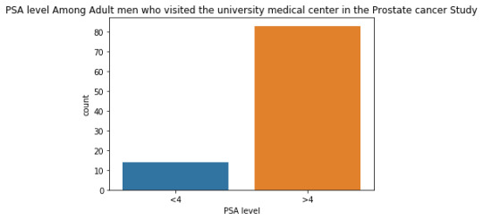
This graph is unimodal, with its highest peak at the  category of >4 PSA level . It seems to be skewed to the left as there are higher frequencies in higher category(>4) than the lower category.

The univariate graph of Age groups:

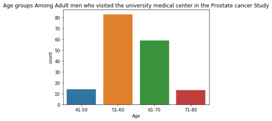
This graph is unimodal, with its highest peak at 51 to 60 age group. It seems to be skewed to the right as there are higher frequencies in the lower age ranges from 51 to 60.

The univariate graph of Cancer Volume:

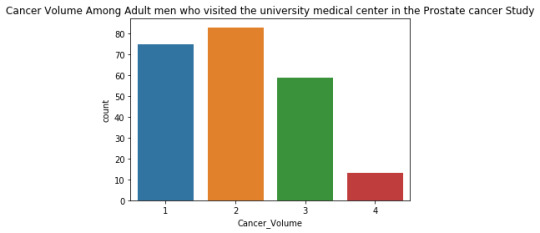
This graph is unimodal, with its highest peak at the  category of 2 (11-20) . It seems to be skewed to the right as there are higher frequencies in lower categories than the higher categories.

The graph above plots the Cancer Volume of the adult men  to the adult men corresponding Age groups. We can see that the bar chat does not show a clear relationship/trend between the two variables.

[beninmondeinfos-blog]

Bénin / Concours à la CNSS : Le cabinet AGEFIC rejette les allégations de Jean-Baptiste Elias - L'info en temps réel sur Bénin Monde Infos http://beninmondeinfos.com/index.php/benin/21-societe/7443-benin-concours-a-la-cnss-accuse-par-anlc-le-cabinet-agefic-se-defend

[my-naomi-blog]

Week 3

import pandas

import numpy

# any additional libraries would be imported here

mydata = pandas.read_csv('prostate_1.csv', low_memory=False)

# subset variables in new data frame, sub1

sub1=mydata[['AgeF','PSA', 'Cancer Volume']]

a = sub1.head

print(a)

#new PSA variable, categorical 1 through 2

def PSA (row):

   if row['PSA'] < 4 :

      return 1

   if row['PSA'] > 4 :

      return 2

sub1['PSA'] = sub1.apply (lambda row: PSA (row),axis=1)

a = sub1.head 

print(a)

#new Age variable, categorical 1 through 2

def Age (row):

   if row['AgeF']== '41-50':

      return 1

   if row['AgeF'] == '51-60' :

      return 2

   if row['AgeF'] == '61-70' :

      return 3

   if row['AgeF'] == '71-80' :

      return 4

sub1['Age'] = sub1.apply (lambda row: Age (row),axis=1)

a = sub1.head 

print(a)

#new Cancer_Volume variable, categorical 1 through 4

def Cancer_Volume(row):

   if row['Cancer Volume'] < 11:

      return 1

   if row['Cancer Volume'] >11 and row['Cancer Volume'] < 21 :

      return 2

   if row['Cancer Volume'] >21 and row['Cancer Volume'] <31 :

      return 3

   if row['Cancer Volume'] >31:

      return 4

sub1['Cancer_Volume'] = sub1.apply (lambda row: Cancer_Volume(row),axis=1)

a = sub1.head 

print(a)

#frequency distributions for primary and secondary ethinciity variables

print( 'counts for PSA level')

c10 = sub1['PSA'].value_counts(sort=False)

print(c10)

print( 'percentages for PSA level')

p10 = sub1['PSA'].value_counts(sort=False, normalize=True)

print (p10)

print('counts for Age')

c11 = sub1['Age'].value_counts(sort=False)

print(c11)

print( 'percentages for Age')

p11= sub1['Age'].value_counts(sort=False, normalize=True)

print (p11)

print( 'counts for Cancer Volume')

c12 = sub1['Cancer_Volume'].value_counts(sort=False)

print(c12)

print( 'percentages for Cancer Volume')

p12 = sub1['Cancer_Volume'].value_counts(sort=False, normalize=True)

print (p12)

Output

runfile('C:/Users/NAOMI/Downloads/Documents/Cousera/Data Visualization/week 3/Assignment 3 new.py', wdir='C:/Users/NAOMI/Downloads/Documents/Cousera/Data Visualization/week 3') <bound method NDFrame.head of      AgeF      PSA  Cancer Volume 0   41-50    0.651         0.5599 1   51-60    0.852         0.3716 2   71-80    0.852         0.6005 3   51-60    0.852         0.3012 4   61-70    1.448         2.1170 ..    ...      ...            ... 92  61-70   80.640        16.9455 93  41-50  107.770        45.6042 94  51-60  170.716        18.3568 95  61-70  239.847        17.8143 96  61-70  265.072        32.1367

[97 rows x 3 columns]> <bound method NDFrame.head of      AgeF  PSA  Cancer Volume 0   41-50    1         0.5599 1   51-60    1         0.3716 2   71-80    1         0.6005 3   51-60    1         0.3012 4   61-70    1         2.1170 ..    ...  ...            ... 92  61-70    2        16.9455 93  41-50    2        45.6042 94  51-60    2        18.3568 95  61-70    2        17.8143 96  61-70    2        32.1367

[97 rows x 3 columns]> <bound method NDFrame.head of      AgeF  PSA  Cancer Volume  Age 0   41-50    1         0.5599    1 1   51-60    1         0.3716    2 2   71-80    1         0.6005    4 3   51-60    1         0.3012    2 4   61-70    1         2.1170    3 ..    ...  ...            ...  ... 92  61-70    2        16.9455    3 93  41-50    2        45.6042    1 94  51-60    2        18.3568    2 95  61-70    2        17.8143    3 96  61-70    2        32.1367    3

[97 rows x 4 columns]> <bound method NDFrame.head of      AgeF  PSA  Cancer Volume  Age  Cancer_Volume 0   41-50    1         0.5599    1              1 1   51-60    1         0.3716    2              1 2   71-80    1         0.6005    4              1 3   51-60    1         0.3012    2              1 4   61-70    1         2.1170    3              1 ..    ...  ...            ...  ...            ... 92  61-70    2        16.9455    3              2 93  41-50    2        45.6042    1              4 94  51-60    2        18.3568    2              2 95  61-70    2        17.8143    3              2 96  61-70    2        32.1367    3              4

[97 rows x 5 columns]> counts for PSA level 1    14 2    83 Name: PSA, dtype: int64 percentages for PSA level 1    0.14433 2    0.85567 Name: PSA, dtype: float64 counts for Age 1     8 2    17 3    59 4    13 Name: Age, dtype: int64 percentages for Age 1    0.082474 2    0.175258 3    0.608247 4    0.134021 Name: Age, dtype: float64 counts for Cancer Volume 1    75 2    16 3     4 4     2 Name: Cancer_Volume, dtype: int64 percentages for Cancer Volume 1    0.773196 2    0.164948 3    0.041237 4    0.020619 Name: Cancer_Volume, dtype: float64

I created new data with  three variables: AgeF, PSA and Cancer Volume. The were no missing data set in my data. For Age, the most commonly endorsed is 3 (60.8%) , meaning  more than half of the  men who went for the checkup are from the age 61-70 years. For PSA, 2 (85.57%) has the highest percentage, meaning the PSA which is greater than 4 has the highest frequency of 83. For Cancer Volume, 1 ( 77.32% ) has the highest percentage among the others which means the Cancer Volume less than 10 has  the highest frequency of 75 with 77.32%.