#Imagen4

[tilbageidanmark]

German Bhangra Remix

[ailatestupdate]

The Gemini Ultra Veo 3 and Imagen 4 are two cutting-edge AI tools making waves in the creative tech space. Gemini Ultra Veo 3 brings advanced video and visual processing capabilities, ideal for high-quality content creation, while Imagen 4 is Google's latest AI image generator known for producing stunningly realistic visuals with impressive detail and speed.

[govindhtech]

Introduce Gemma 3n preview, Veo 3, Imagen 4 & Veo 2 updates

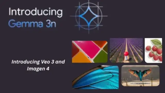
New Google AI Models and Tools Advance Creative Media Creation and On-Device AI

Google has announced numerous new models and tools that emphasise advanced generative media production and on-device capabilities to make AI more accessible.

Gemma 3n

Gemma 3n preview, a powerful, mobile-first AI model, is important. Gemma 3n, the first open model with a new architecture, was developed with Qualcomm Technologies, MediaTek, and Samsung System LSI. This architecture is optimised for rapid, multimodal AI to enable truly private and intimate interactions on computers, tablets, and phones.

Gemma 3n's main features:

Compared to Gemma 3 4B, it reacts 1.5 times faster on mobile devices, has better quality, and uses less memory. Per-Layer Embeddings (PLE) reduces RAM usage and allows models with 5B and 8B parameter counts to work with a dynamic memory footprint of ONLY 2GB and 3GB.

MatFormer training allows a 4B active memory footprint model to natively incorporate a layered state-of-the-art 2B active memory footprint submodel. This lets you dynamically balance quality and performance. We add mix-and-match capability to the 4B model to dynamically construct submodels for certain use scenarios.

Privacy-First & Offline Ready: Local execution enables features that safeguard user privacy and work offline.

Gemma 3n understands text, sounds, and visuals well and has excellent video understanding. Audio features include high-quality Automatic Speech Recognition and Translation. Accepting interleaved data from multiple modalities lets it understand complex relationships.

It performs better overall, but best in Japanese, German, Korean, Spanish, and French.

Gemma 3n gives an early peek at Android and Chrome's architectural breakthroughs with the Gemini Nano generation, which will be powered by this same architecture and released later this year. Google AI Edge for on-device development and Google AI Studio for cloud-based research allow developers to preview Gemma 3n today.

Google is releasing new generative media tools and models in addition to on-device improvements. These aim to empower artists and producers by pushing media generation.

The updated and new creative tools are:

Veo 3: A revolutionary video-making model that records speech, traffic, and bird sounds. It works in text and image prompting, lip syncing, and physics. Enterprise users can use Veo 3 on Vertex AI, while US Ultra subscribers can use Gemini and Flow.

Veo 2 updates: Creator feedback led to object add/remove capability, camera controls for precise movements, outpainting to extend the frame, and state-of-the-art reference-powered video for creative control and consistency. Flow has reference-powered camera and video controllers.

Flow: A Veo-specific AI filmmaking tool for creatives. Flow lets users create cinematic scenes, clips, and narratives using Google DeepMind's most advanced models (Veo, Imagen, and Gemini). Users can describe photos in plain language and manage plot elements. Google AI Pro and Ultra US subscribers can now use Flow.

Imagen 4, the latest model, produces gorgeous images with great typography quickly and accurately. Imagen 4 supports aspect ratios up to 2k, has enhanced typeface and spelling, has excellent detail clarity, and works well in many styles. The Gemini app, Whisk, and Vertex AI offer it with Workspace apps like Slides, Vids, and Docs. A faster version is coming.

Lyria 2: This music creation paradigm now allows unlimited research and innovation. Businesses may employ Vertex AI and creators can use Lyria 2. AI Studio and API access MusicFX DJ's interactive music composition model, Lyria RealTime.

Google emphasises responsible AI development. SynthID watermarks will help identify Veo 3, Imagen 4, and Lyria 2 outputs as AI-generated. This watermark-based verification gateway, SynthID Detector, is unveiled today to help consumers recognise AI-generated content. As AI advances, Google is apprehensive of open models and strives to enhance protocols. It aims to unleash creativity and help creators realise their ideas.

[mmm-plts]

Variable moderadora Cráteres en Marte

Luego del análisis de los datos de los Cráter en Marte una variable moderadora puede ser la ubicación (Latitud, Longitud) en relación con la profundidad y el diámetro. Les comparto mi código y los resultados:

Código

import numpy as np import pandas import statsmodels.formula.api as smf import scipy from scipy import stats from scipy.stats import pearsonr import seaborn import matplotlib.pyplot as plt

data = pandas.read_csv('marscrater_pds.csv', low_memory=False) data['LATITUDE_CIRCLE_IMAGE']=pandas.to_numeric(data['LATITUDE_CIRCLE_IMAGE']) data['LONGITUDE_CIRCLE_IMAGE']=pandas.to_numeric(data['LONGITUDE_CIRCLE_IMAGE']) data['DIAM_CIRCLE_IMAGE']=pandas.to_numeric(data['DIAM_CIRCLE_IMAGE']) data['NUMBER_LAYERS']=pandas.to_numeric(data['NUMBER_LAYERS']) data['DEPTH_RIMFLOOR_TOPOG']=pandas.to_numeric(data['DEPTH_RIMFLOOR_TOPOG'])

#Se escribe de la siguiente manera el código

# modelname =smf.ols(formula='QUANT_RESPONSE ~ C(CAT_EXPLANATORY)', data=dataframe.fit())

# print(modelname.symary())

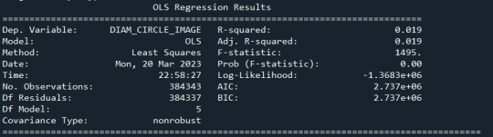
model1=smf.ols(formula='NUMBER_LAYERS ~ C(LATITUDE_CIRCLE_IMAGE)',data=data).fit()

print(model1.sumary())

Relaciono por cantidad de cortes

sub1=data[(data['DIAM_CIRCLE_IMAGE']>=0) & (data['DIAM_CIRCLE_IMAGE']<=70000)] cut0 =data[(data['NUMBER_LAYERS']==0)] cut1 =data[(data['NUMBER_LAYERS']==1)] cut2 =data[(data['NUMBER_LAYERS']==2)] cut3 =data[(data['NUMBER_LAYERS']==3)] cut4 =data[(data['NUMBER_LAYERS']==4)] cut5 =data[(data['NUMBER_LAYERS']==5)]

using ols function for calculating the F-statistic and associated p value

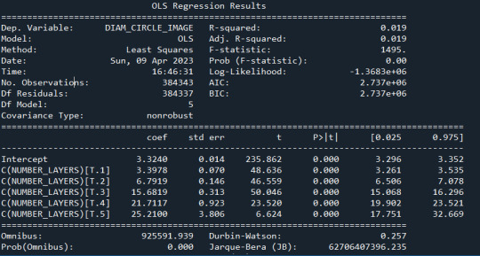
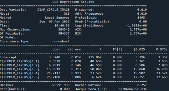
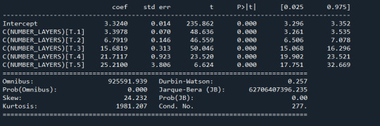
model1 = smf.ols(formula='DIAM_CIRCLE_IMAGE ~ C(NUMBER_LAYERS)', data=sub1) results1 = model1.fit() print ("Modelo OLS de Diámetro y Número de capas \n" , results1.summary())

Con los cortes hice nuevos dataframe por cada capa, análizo los resultados

de cada capa y comaparó la capa uno con la cero

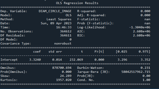
model2 = smf.ols(formula='DIAM_CIRCLE_IMAGE ~ C(NUMBER_LAYERS)', data=cut0) results2 = model2.fit() print ("Modelo OLS de Diámetro y Cero capas \n", results2.summary())

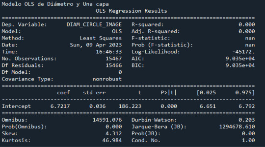
model3 = smf.ols(formula='DIAM_CIRCLE_IMAGE ~ C(NUMBER_LAYERS)', data=cut1) results3 = model3.fit() print ("Modelo OLS de Diámetro y Una capa \n", results3.summary())

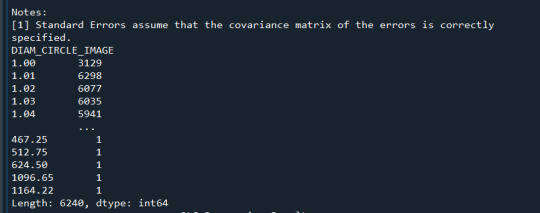
ct1 = sub1.groupby('DIAM_CIRCLE_IMAGE').size() print (ct1)

using ols function for calculating the F-statistic and associated p value

model1 = smf.ols(formula='DIAM_CIRCLE_IMAGE ~ C(NUMBER_LAYERS)', data=sub1) results1 = model1.fit() print (results1.summary())

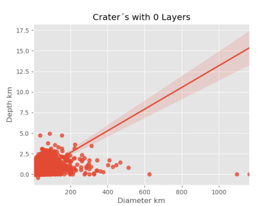
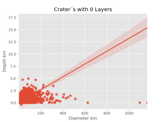
imagen0=seaborn.regplot(x=cut0['DIAM_CIRCLE_IMAGE'], y =cut0['DEPTH_RIMFLOOR_TOPOG'], fit_reg = True, data = cut0) plt.xlabel("Diameter km") plt.ylabel("Depth km") plt.title("Crater´s with 0 Layers") plt.show()

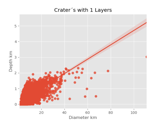
imagen1=seaborn.regplot(x=cut1['DIAM_CIRCLE_IMAGE'], y =cut1['DEPTH_RIMFLOOR_TOPOG'], fit_reg = True, data = cut1) plt.xlabel("Diameter km") plt.ylabel("Depth km") plt.title("Crater´s with 1 Layers")

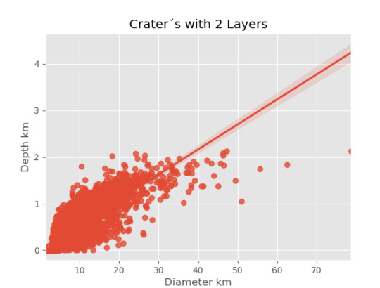
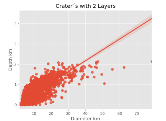
imagen2=seaborn.regplot(x=cut2['DIAM_CIRCLE_IMAGE'], y =cut2['DEPTH_RIMFLOOR_TOPOG'], fit_reg = True, data = cut2) plt.xlabel("Diameter km") plt.ylabel("Depth km") plt.title("Crater´s with 2 Layers")

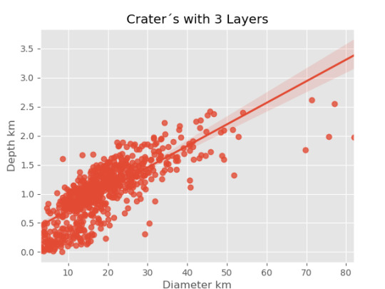
imagen3=seaborn.regplot(x=cut3['DIAM_CIRCLE_IMAGE'], y =cut3['DEPTH_RIMFLOOR_TOPOG'], fit_reg = True, data = cut3) plt.xlabel("Diameter km") plt.ylabel("Depth km") plt.title("Crater´s with 3 Layers")

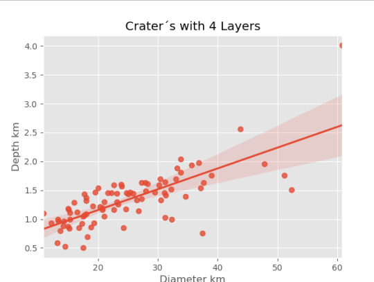
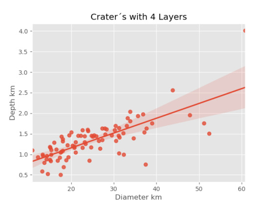
imagen4=seaborn.regplot(x=cut4['DIAM_CIRCLE_IMAGE'], y =cut4['DEPTH_RIMFLOOR_TOPOG'], fit_reg = True, data = cut4) plt.xlabel("Diameter km") plt.ylabel("Depth km") plt.title("Crater´s with 4 Layers")

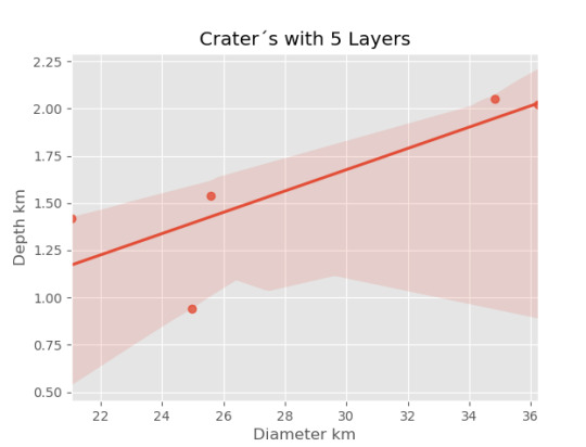
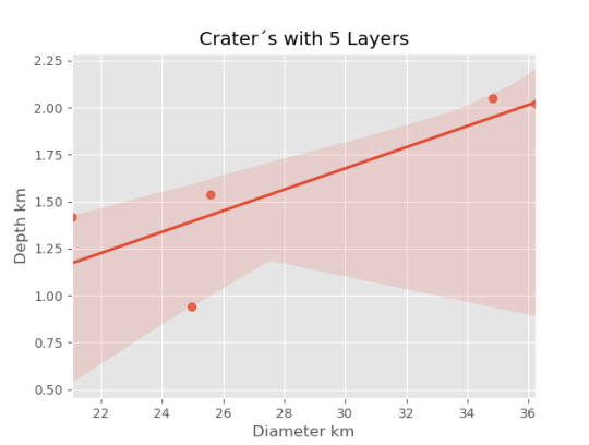
imagen5=seaborn.regplot(x=cut5['DIAM_CIRCLE_IMAGE'], y =cut5['DEPTH_RIMFLOOR_TOPOG'], fit_reg = True, data = cut5) plt.xlabel("Diameter km") plt.ylabel("Depth km") plt.title("Crater´s with 5 Layers")

Resultados

[ladyeskeleto-blog]

imagen1:cristal sans (guardian de multitale)

imagen2:la ruta genosida

imagen3: gaster y agatta (padres de g-dream y g-nightmer)

imagen4:gaster dream

imagen5:multi error (reset guardian de multitale)

imagen6:los hijos de lady y jammy

[nikifiser]

Glitch-art - Serie3 - Audacity - Imagen4 

[integralarchitecturestudio]

VISITA DE OBRA - VIVIENDA ADOSADA EN CEUTÍ

VISITA DE OBRA – VIVIENDA ADOSADA EN CEUTÍ

Montaje del encofrado del forjado de planta baja. Hormigonado de rampa de acceso de vehículos y rampa accesible para personas.

Imagen1.

Imagen2.

Imagen3.

Imagen4.

[hyoga2k]

¿Y si votamos por internet?

¿Y si votamos por internet?

Siempre se ha propuesto la implementación del voto electrónico en Chile. Y es que la incomodidad de salir de la casa en un día “feriado”, hacer la fila, el “riesgo” de quedar como vocal de mesa y otras situaciones similares, si tan solo pudiéramos votar haciendo clic en la pantalla del computador o el smartphone. También es cierto que desde hace más o menos 10 años, el gobierno chileno lleva…

[anuncialovenezuela-blog]

Zapatillas tipo Cocuizas excelente calidad al mejor precio - AnuncialoVenezuela.com

ZAPATILLAS TIPO COCUIZAS EXCELENTE CALIDAD AL MÁS BAJO PRECIO DEL MERCADO

IMAGEN 1 Y 2: TALLA38

IMAGEN3: TALLA39

IMAGEN4 Y 5: TALLA 40 Y 41

IMAGEN 6: TALLA 37

HAGO ENTREGAS PERSONALES EN LA CIUDAD DE VALENCIA, SAN DIEGO, LOS GUAYOS, NAGUANAGUA A TU SERVICIO.  TAN SOLO 16.000BS MAYOR INFORMACIÓN A TRAVÉS DE LA PAGINA OFICIAL► https://www.facebook.com/modaligeraparatuspies/

  Para ver el anuncio completo visita la pagina:

http://www.anuncialovenezuela.com/zapatillas-tipo-cocuizas-excelente-calidad-al-mejor-precio/

  #Venezuela #ANUNCIALOVENEZUELA

  #ZapatosyAccesorios

[mmm-plts]

ANOVA Cráteres en Marte

Comparto los resultados de mi análisis con ANOVA, donde obtengo la correlación de Pearson , para la relación de diámetro y profundidad según la cantidad de capaz captadas en los datos.

El código es:

-- coding: utf-8 --

""" Created on Mon Mar 13 09:32:30 2023

@author: ANGELA """

import numpy import pandas import statsmodels.formula.api as smf import statsmodels.stats.multicomp as multi import seaborn import scipy from scipy import stats from scipy.stats import pearsonr import matplotlib.pyplot as plt

Configuración matplotlib

plt.style.use('ggplot')

def funtion_plot(val_x,val_y, title): # relación entre diametro del crater cob la profundidad plt = seaborn.regplot(x=val_x, y =val_y, fit_reg = True, data = data) plt.xlabel("km") plt.ylabel (" km") plt.title(title) plt.show()

data = pandas.read_csv('marscrater_pds.csv', low_memory=False)

data['LATITUDE_CIRCLE_IMAGE']=pandas.to_numeric(data['LATITUDE_CIRCLE_IMAGE']) data['LONGITUDE_CIRCLE_IMAGE']=pandas.to_numeric(data['LONGITUDE_CIRCLE_IMAGE']) data['DIAM_CIRCLE_IMAGE']=pandas.to_numeric(data['DIAM_CIRCLE_IMAGE']) data['NUMBER_LAYERS']=pandas.to_numeric(data['NUMBER_LAYERS']) data['DEPTH_RIMFLOOR_TOPOG']=pandas.to_numeric(data['DEPTH_RIMFLOOR_TOPOG'])

funtion_plot(data['DIAM_CIRCLE_IMAGE'], data['DEPTH_RIMFLOOR_TOPOG'])

Relaciono por cantidad de cortes

Sub1=data[(data['DIAM_CIRCLE_IMAGE']>=0) & (data['DIAM_CIRCLE_IMAGE']<=70000)]

cut0 =data[(data['NUMBER_LAYERS']==0)] cut1 =data[(data['NUMBER_LAYERS']==1)] cut2 =data[(data['NUMBER_LAYERS']==2)] cut3 =data[(data['NUMBER_LAYERS']==3)] cut4 =data[(data['NUMBER_LAYERS']==4)] cut5 =data[(data['NUMBER_LAYERS']==5)]

print("Relation depth and diameter") print(scipy.stats.pearsonr(cut0['DIAM_CIRCLE_IMAGE'], cut0['DEPTH_RIMFLOOR_TOPOG']), 'Pearsons with 0 layer') print(scipy.stats.pearsonr(cut1['DIAM_CIRCLE_IMAGE'], cut1['DEPTH_RIMFLOOR_TOPOG']), 'Pearsons with 1 layer') print(scipy.stats.pearsonr(cut2['DIAM_CIRCLE_IMAGE'], cut2['DEPTH_RIMFLOOR_TOPOG']), 'Pearsons with 2 layer') print(scipy.stats.pearsonr(cut3['DIAM_CIRCLE_IMAGE'], cut3['DEPTH_RIMFLOOR_TOPOG']), 'Pearsons with 3 layer') print(scipy.stats.pearsonr(cut4['DIAM_CIRCLE_IMAGE'], cut4['DEPTH_RIMFLOOR_TOPOG']), 'Pearsons with 4 layer') print(scipy.stats.pearsonr(cut5['DIAM_CIRCLE_IMAGE'], cut5['DEPTH_RIMFLOOR_TOPOG']), 'Pearsons with 5 layer')

imagen0=seaborn.regplot(x=cut0['DIAM_CIRCLE_IMAGE'], y =cut0['DEPTH_RIMFLOOR_TOPOG'], fit_reg = True, data = cut0) plt.xlabel("Diameter km") plt.ylabel("Depth km") plt.title("Crater´s with 0 Layers") plt.show()

imagen1=seaborn.regplot(x=cut1['DIAM_CIRCLE_IMAGE'], y =cut1['DEPTH_RIMFLOOR_TOPOG'], fit_reg = True, data = cut1) plt.xlabel("Diameter km") plt.ylabel("Depth km") plt.title("Crater´s with 1 Layers")

imagen2=seaborn.regplot(x=cut2['DIAM_CIRCLE_IMAGE'], y =cut2['DEPTH_RIMFLOOR_TOPOG'], fit_reg = True, data = cut2) plt.xlabel("Diameter km") plt.ylabel("Depth km") plt.title("Crater´s with 2 Layers")

imagen3=seaborn.regplot(x=cut3['DIAM_CIRCLE_IMAGE'], y =cut3['DEPTH_RIMFLOOR_TOPOG'], fit_reg = True, data = cut3) plt.xlabel("Diameter km") plt.ylabel("Depth km") plt.title("Crater´s with 3 Layers")

imagen4=seaborn.regplot(x=cut4['DIAM_CIRCLE_IMAGE'], y =cut4['DEPTH_RIMFLOOR_TOPOG'], fit_reg = True, data = cut4) plt.xlabel("Diameter km") plt.ylabel("Depth km") plt.title("Crater´s with 4 Layers")

imagen5=seaborn.regplot(x=cut5['DIAM_CIRCLE_IMAGE'], y =cut5['DEPTH_RIMFLOOR_TOPOG'], fit_reg = True, data = cut5) plt.xlabel("Diameter km") plt.ylabel("Depth km") plt.title("Crater´s with 5 Layers")

Los resultados son:

El calculo de la relación de Pearson por la cantidad de capaz es

Los resultados gráficos son: