#Worksheet_SelectionChange

[fernando-arciniega]

Ajustar automáticamente las columnas en Excel son un simple código

¡El Atajo Secreto Revelado! 🤫 Autoajuste de Columnas con un Toque Mágico ✨

Ya vimos lo útil que es el autoajuste, pero ¿y si te dijera que puedes tener ese poder al alcance de un par de clics sin necesidad de menús? ¡Así es! Excel nos permite usar un pequeño fragmento de código VBA (Visual Basic for Applications) para automatizar tareas, ¡y el autoajuste de columnas no es la excepción! 🧙‍♂️ ¿Cómo funciona esta magia? 🤔 Vamos a insertar un código directamente en tu hoja de cálculo que se activará cada vez que cambies de celda, ajustando automáticamente el ancho de todas las columnas para que el contenido se vea perfecto. ¡Es como tener un asistente personal de formato! 🤖 ¡Paso a Paso Hacia la Automatización! 🚀 Sigue estos sencillos pasos para activar el autoajuste automático en tu hoja de cálculo: - Abre tu hoja de cálculo de Excel. 📂 ¡La que quieres tener siempre impecable! 😉 - Haz clic derecho en cualquier lugar de la hoja de cálculo. 🖱️ Se abrirá un menú contextual. - Selecciona la opción "Ver Código". ⚙️ Esto abrirá el editor de VBA. ¡No te asustes! Parece complejo, pero solo vamos a pegar unas líneas. 🤓

- En la ventana del editor de VBA, busca en el panel de la izquierda el nombre de tu hoja de cálculo. Debería aparecer algo como "Hoja1 (NombreDeTuHoja)". Haz doble clic sobre él. 👆👆 Si no tiene nombre aparece como Worksheet

- Se abrirá una ventana de código en blanco. Aquí es donde vamos a pegar el código mágico. ✨ - Copia y pega el siguiente código exactamente como aparece: 📝 - Tienes que agregar solo: - Cells.EntireColumn.AutoFit

- ¡Listo! Cierra la ventana del editor de VBA. ❌ ¿Y ahora qué? 🤔 ¡Ahora, cada vez que hagas clic en una celda diferente dentro de esa hoja de cálculo, Excel automáticamente ajustará el ancho de todas las columnas para mostrar todo el contenido correctamente! ¡Adiós a las columnas cortadas o demasiado anchas! 👋 ¡Es como magia en tiempo real! 🧙‍♀️

Consideraciones Importantes 🤔 Si bien este método es súper rápido y cómodo, recuerda lo que mencionamos antes: - Rendimiento: En hojas de cálculo muy grandes, este autoajuste constante podría consumir recursos y hacer que Excel se sienta un poco más lento. 🐢 - Interrupciones: Si estás intentando ajustar manualmente el ancho de una columna, este código lo sobrescribirá cada vez que cambies de selección. 😬 Si estos puntos te preocupan, quizás prefieras usar el método del doble clic en los encabezados o crear un botón para autoajustar cuando lo necesites. ¡La flexibilidad es clave! 🔑 Aun así, para muchas situaciones, este pequeño truco de VBA puede ser una verdadera joya para mantener tus hojas de cálculo siempre ordenadas y legibles sin esfuerzo. ¡Pruébalo y cuéntanos qué tal te funciona! 😊 Read the full article

[hiyoko-channnel]

こんなExcelは嫌だ！【イベントマクロの紹介】

麗かな音楽にのせて、イベントマクロのご紹介～！ 初めてこれを知った時は感動しました。 0:00　Worksheet_SelectionChange イベント 1:57　Worksheet_Change イベント 3:57　WorkBook_Open イベント 5:58　WorkBook_NewSheet イベント ＜Twitter＞ わちょん ＜チャンネル紹介＞ ExcelやVBA中心。時には真剣に、時には楽しく【ゆっくり動画】を作っています ＜動画編集ソフト＞ ゆっくりMovieMaker4 ＜音楽・効果音＞ 甘茶の音楽工房 さん 効果音ラボ…

[greysgiga]

Compare two columns in excel and return differences

#Compare two columns in excel and return differences update

#Compare two columns in excel and return differences code

#Compare two columns in excel and return differences update

I am in the middle of taking it out and prepping it for deployment as it was bought as a spare, and a switch is failing calling for it to be replaced. I have configured it but I want to update the firmware. I have a HP Procurve 2920 Switch (Bought 2010). Will my HP Procurve Take Aruba firmware? Hardware.It is provided as an example and a starting point for your development.

#Compare two columns in excel and return differences code

This is Air Code - I have neither compiled nor tested it. Private Sub Worksheet_SelectionChange(ByVal Target As Range) Why did I write this as a separate procedure (rather than, for example, the Worksheet_Change event procedure on the worksheet)? Well, we want to call this procedure whenever something changes on either worksheet so we can share this procedure by coding each worksheet's Worksheet_Change event procedure like this: You can use the Worksheet.Change event to call this procedure. So, when should this procedure be called? I would suggest calling it every time any value on either of the two worksheets changes. ' the colors in case the row was marked asįirstSheet.Range(Cells(index1, 1), Cells(index1, 4)).Interior.Color = vbWhiteįirstSheet.Range(Cells(index1, 1), Cells(index1, 4)).Font.Color = vbBlackįirstSheet.Range(Cells(index1, 1), Cells(index1, 4)).Interior.Color = vbYellowįirstSheet.Range(Cells(index1, 1), Cells(index1, 4)).Font.Color = vbRed ' the two sheets change, so we need to RESET ' to be called repeatedly as the values on ' (We do this because we expect this procedure ' If we DIDN'T find a match, we want to mark ' We've found a row on the second sheet that & secondSheet.Cells(index2, SECONDCOLUMN2) SecondValue = secondSheet.Cells(index2, FIRSTCOLUMN2) _ ' Loop through the rows on the second sheet ' Keep track of whether we've found a match & firstSheet.Cells(index1, SECONDCOLUMN1) ' For each row, concatenate the values from the two cellsįirstValue = firstSheet.Cells(index1, FIRSTCOLUMN1) _ ' Loop through the rows on the first worksheet Set secondSheet = ActiveWorkbook.Sheets(secondSheetName) Set firstSheet = ActiveWorkbook.Sheets(firstSheetName) Public Sub CompareSheets(firstSheetName As String, secondSheetName As String) The procedure looks like this:Ĭonst FIRSTCOLUMN1 As Integer = 2 'Column BĬonst SECONDCOLUMN1 As Integer = 3 'Column CĬonst FIRSTCOLUMN2 As Integer = 1 'Column AĬonst SECONDCOLUMN2 As Integer = 3 'Column C Whenever a row on the first sheet fails to have a match somewhere on the second sheet, this procedure will change the colors of the row to make its error status visible. I've put together some code that will perform this process. The procedure (I prefer not to use the term "macro" because in Excel that can, and should, refer to an MS Excel 4.0 Macro, which is a completely different and much uglier beast) will need to have two nested loops: an outer loop to scan the rows on the first sheet, and an inner loop to scan the rows on the second sheet. You have correctly concluded that you will need to use VBA to fulfill your requirements. However, let's ignore that and try to come up with an answer to your question. As John has pointed out, this thread is in the wrong forum - it should be in the Visual Basic for Applications (VBA) forum ( http:/ / / groups/ technical-functional/ vb-vba-l) rather than the SQL Server forum ( http:/ / / groups/ technical-functional/ sql-server-l).

[exctips]

Macro en Excel para remarcar la fila y columna sobre la que se posiciona el cursor y construir un minigráfico con la información de la fila.:

'##### remarca la línea y la columna en que se posiciona el cursor (celda activa)} '##### NO afecta los formatos condicionales

Private Sub Worksheet_SelectionChange(ByVal Target As Range)

   Dim x As Integer    Dim TotShapes As Integer

   Dim RutaArchivo As String    Dim NombreLibro As String    Dim NombreHoja As String

   Dim ColIni As Integer    Dim ColFin As Integer    Dim FilIni As Integer    Dim FilFin As Integer    Dim Fil As Integer    Dim Col As Integer    Dim FilEncabeza As Integer    Dim FilIniLet As String    Dim FilFinLet As String

   Dim Rango As Range

   '#### Se definen la Columna Inicial, Columna Final, Fila Inicial y Fila Final del rango a activar    '#### Fila de encabezado para eje x del gráfico    ColIni = 3    ColFin = 14    FilIni = 3    FilFin = 7    FilEncabeza = 1

   '##### Limpia el patrón del rango de trabajo

   '##### Obtiene fila y columna de la celda activa    Fil = ActiveCell.Row    Col = ActiveCell.Column    '##### Se ejecuta solo en el rango de trabajo    If Fil >= FilIni And Fil <= FilFin And Col >= ColIni And Col <= ColFin Then

      RutaArchivo = ActiveWorkbook.Path + "\"       NombreLibro = ActiveWorkbook.Name       NombreHoja = ActiveSheet.Name

      '### Limpia el patrón anterior en el rango       Range(Cells(FilIni, ColIni), Cells(FilFin, ColFin)).Interior.Pattern = xlNone

      '### Covierte números de columnas en sus respectivas letras       ColIniLet = ConvertToLetter(ColIni)       ColFinLet = ConvertToLetter(ColFin)

      '### Define el rango seleccionado (fila completa)       NomRango = ColIniLet + Trim(Str(Fil)) + ":" + ColFinLet + Trim(Str(Fil))       Set Rango = Worksheets(NombreHoja).Range(NomRango)

      '### Limpia minigráficos anteriores        Cells(FilIni + 1, ColFin + 2).Select        Selection.SparklineGroups.Clear

      '#### Construye el título del gráfico con los encabezados de fila       tex = Trim(Cells(Fil, 1).Value)       '#### Coloca el nobre del gráfico       Cells(3, ColFin + 2).Value = tex       '#### Pone en gris la fila y la columna activas       Range(Cells(Fil, ColIni), Cells(Fil, ColFin)).Interior.ColorIndex = 15       Range(Cells(FilIni, Col), Cells(FilFin, Col)).Interior.ColorIndex = 15

      '###Construye minigráfico       Cells(FilIni + 1, ColFin + 2).SparklineGroups.Add Type:=xlSparkLine, SourceData:=NomRango

   End If

End Sub

Function ConvertToLetter(iCol As Integer) As String '### Convierte números de columnas en su respectiva letra. '###Fuente: https://support.microsoft.com/en-us/help/833402/how-to-convert-excel-column-numbers-into-alphabetical-characters   Dim iAlpha As Integer   Dim iRemainder As Integer   iAlpha = Int(iCol / 27)   iRemainder = iCol - (iAlpha * 26)   If iAlpha > 0 Then      ConvertToLetter = Chr(iAlpha + 64)   End If   If iRemainder > 0 Then      ConvertToLetter = ConvertToLetter & Chr(iRemainder + 64)   End If End Function

[googleexcel]

MAKE ANY USERFORM

Dim CurRow As Long

Private Data(9, 3) As String

Private Type DispS   Top As Double   Left As Double End Type Dim DispStru(10) As DispS Dim DispRatio As Double

Const ScreenWidth = 9000   '8 Const ScreenHeight = 12000  '12

Private Sub CommandButton1_Click() ' UserForm1.Width If CurRow < 3 Then   CurRow = 3 End If

UserForm1.adil.Caption = Sheet1.Cells.Item(CurRow, 2).Value UserForm1.india.Caption = Sheet1.Cells.Item(CurRow, 3).Value

DispStru(2).Top = Sheet1.Cells.Item(2, 13).Value DispStru(2).Left = Sheet1.Cells.Item(2, 14).Value

DispStru(3).Top = Sheet1.Cells.Item(3, 13).Value DispStru(3).Left = Sheet1.Cells.Item(3, 14).Value

'DispRatio = ((9 * 9) / 8) * 1000

DispRatio = 71.43    '50

UserForm1.adil.Top = DispStru(2).Top * DispRatio UserForm1.adil.Left = DispStru(2).Left * DispRatio

UserForm1.india.Top = DispStru(3).Top * DispRatio UserForm1.india.Left = DispStru(3).Left * DispRatio 'UserForm1.Width = 9000 UserForm1.Top = 0 UserForm1.Left = 0 UserForm1.Show vbModal

End Sub

Private Sub Worksheet_SelectionChange(ByVal Target As Range) 'UserForm1.Show 'Sheet1.Cells.Item(i, 11).Value   CurRow = Target.Cells.Row If CurRow < 3 Then   CurRow = 3 End If

Sheet1.Cells.Item(2, 9).Value = Sheet1.Cells.Item(CurRow, 2).Value Sheet1.Cells.Item(3, 9).Value = Sheet1.Cells.Item(CurRow, 3).Value Sheet1.Cells.Item(4, 9).Value = Sheet1.Cells.Item(CurRow, 4).Value

'MsgBox CurRow

End Sub

[minikarpuz]

Excel Seçili Satırı Renklendirme

Excel’de birbirinden uzak sütunlardaki bilgileri okurken gözümüz farkında olmadan bir başka satırın bilgilerini okuyor olabilir. Bunu engellemek için seçili hücrenin bulunduğu satırı renklendirmek güzel bir yöntem diye düşünüyorum. 

Yöntemi uygulamak için Excel çalışma sayfasında Geliştirici sekmesine tıklayın. Burada Visual Basic kodlarına aşağıdaki kodları yapıştırın. 

Private Sub Worksheet_SelectionChange(ByVal Target As Range) Cells.Interior.ColorIndex = xlNone If Intersect(Target, [A1:Q1000]) Is Nothing Then Exit Sub Range(Cells(Target.Row, 1), Cells(Target.Row, 17)).Interior.ColorIndex = 6 End Sub

[fernando-arciniega]

Ajusta automáticamente el tamaño de las Celdas en Excel con este truco

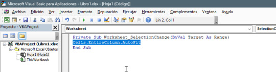
En Excel, es común encontrarse con hojas de cálculo extensas que contienen datos en varias columnas. A veces, el ancho predeterminado de las columnas no es suficiente para mostrar todos los datos de manera adecuada, lo que puede resultar en la incomodidad de tener que desplazarse horizontalmente. Afortunadamente, Excel nos brinda una solución para este problema al permitirnos ajustar automáticamente el ancho de columna al seleccionar una celda específica. En esta entrada de blog, te mostraré cómo lograrlo utilizando una macro en VBA. Explicación de la macro: La macro en cuestión se activa cada vez que se produce un cambio de selección en la hoja de cálculo. Esto significa que cuando seleccionas una celda distinta, Excel ejecutará automáticamente el código VBA contenido en esta macro. Aquí está la macro: Private Sub Worksheet_SelectionChange(ByVal Target As Range) Cells.EntireColumn.AutoFit End Sub La línea de código Private Sub Worksheet_SelectionChange(ByVal Target As Range) indica que esta macro se aplica a la hoja de cálculo actual y se activa cuando ocurre un cambio de selección. La línea Cells.EntireColumn.AutoFit es la acción que se realiza cada vez que ocurre un cambio de selección. La propiedad EntireColumn se refiere a la columna completa que contiene la celda seleccionada. La función AutoFit ajusta automáticamente el ancho de la columna para que se ajuste al contenido de la celda más ancha en esa columna. Esto garantiza que todos los datos de la columna sean visibles sin tener que desplazarse horizontalmente.

Cómo insertar el código de la macro en Excel

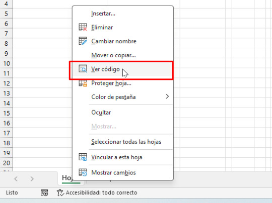
Haz clic con el botón derecho sobre la hoja en la que deseas que se ajuste automáticamente las celdas, luego selecciona la opción "ver código".

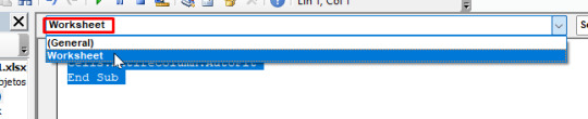
Despliega las opciones del menú, y selecciona "Worksheet" ahí, deberás escribir: Cells.EntireColumn.AutoFit Escríbelo entre las líneas que se muestran por default, para que al final quede así:

Recuerda que esta macro se aplicará a la hoja de cálculo específica en la que la hayas insertado. Si deseas aplicarla a otras hojas, deberás copiarla y pegarla en cada una de ellas. Espero que esta explicación te haya sido útil. Si tienes alguna otra pregunta, no dudes en hacerla. ¡Buena suerte con tus hojas de cálculo en Excel! Aquí te dejo el video explicativo: https://youtube.com/shorts/xykZ-1Xp7jE?feature=share Read the full article

[hiyoko-channnel]

こんなExcelは嫌だ！【イベントマクロの紹介】

麗かな音楽にのせて、イベントマクロのご紹介～！ 初めてこれを知った時は感動しました。 0:00　Worksheet_SelectionChange イベント 1:57　Worksheet_Change イベント 3:57　WorkBook_Open イベント 5:58　WorkBook_NewSheet イベント ＜Twitter＞ わちょん ＜チャンネル紹介＞ ExcelやVBA中心。時には真剣に、時には楽しく【ゆっくり動画】を作っています ＜動画編集ソフト＞ ゆっくりMovieMaker4 ＜音楽・効果音＞ 甘茶の音楽工房 さん 効果音ラボ…

[hiyoko-channnel]

こんなExcelは嫌だ！【イベントマクロの紹介】

麗かな音楽にのせて、イベントマクロのご紹介～！ 初めてこれを知った時は感動しました。 0:00　Worksheet_SelectionChange イベント 1:57　Worksheet_Change イベント 3:57　WorkBook_Open イベント 5:58　WorkBook_NewSheet イベント ＜Twitter＞ わちょん ＜チャンネル紹介＞ ExcelやVBA中心。時には真剣に、時には楽しく【ゆっくり動画】を作っています ＜動画編集ソフト＞ ゆっくりMovieMaker4 ＜音楽・効果音＞ 甘茶の音楽工房 さん 効果音ラボ…

[googleexcel]

MOUSE CLICK EVENT

Private Sub Worksheet_SelectionChange(ByVal Target As Range) If Target.Address = Range("B5").Address Then Range("B5").Value = "AXIS" End Sub

[googleexcel]

Track

Dim vOldVal 'Must be at top of module Private Sub Worksheet_Change(ByVal Target As Range) Dim bBold As Boolean If Target.Cells.Count > 1 Then Exit Sub On Error Resume Next With Application .ScreenUpdating = False .EnableEvents = False End With If IsEmpty(vOldVal) Then vOldVal = "Empty Cell" bBold = Target.HasFormula With Sheet2 .Unprotect Password:="Secret" If .Range("A1") = vbNullString Then .Range("A1:E1") = Array("CELL CHANGED", "OLD VALUE", _ "NEW VALUE", "TIME OF CHANGE", "DATE OF CHANGE") End If With .Cells(.Rows.Count, 1).End(xlUp)(2, 1) .Value = Target.Address .Offset(0, 1) = vOldVal With .Offset(0, 2) If bBold = True Then .ClearComments .AddComment.Text Text:= _ "OzGrid.com:" & Chr(10) & "" & Chr(10) & _ "Bold values are the results of formulas" End If .Value = Target .Font.Bold = bBold End With .Offset(0, 3) = Time .Offset(0, 4) = Date End With .Cells.Columns.AutoFit .Protect Password:="Secret" End With vOldVal = vbNullString With Application .ScreenUpdating = True .EnableEvents = True End With On Error GoTo 0 End Sub Private Sub Worksheet_SelectionChange(ByVal Target As Range) vOldVal = Target End Sub

[googleexcel]

Macro button scroll down stop

Private Sub Worksheet_SelectionChange(ByVal Target As Range) With ActiveWindow.VisibleRange ActiveSheet.Shapes("CommandButton1").Top = .Top ActiveSheet.Shapes("CommandButton1").Left = .Left End With End Sub

[googleexcel]

tracking sheets

Dim vOldVal 'Must be at top of module Private Sub Worksheet_Change(ByVal Target As Range) Dim bBold As Boolean

If Target.Cells.Count > 1 Then Exit Sub On Error Resume Next

   With Application    .ScreenUpdating = False    .EnableEvents = False    End With

   If IsEmpty(vOldVal) Then vOldVal = "Empty Cell"    bBold = Target.HasFormula    With Sheet2        .Unprotect Password:="Secret"        If .Range("A1") = vbNullString Then            .Range("A1:E1") = Array("CELL CHANGED", "OLD VALUE", _            "NEW VALUE", "TIME OF CHANGE", "DATE OF CHANGE")        End If

       With .Cells(.Rows.Count, 1).End(xlUp)(2, 1)        .Value = Target.Address        .Offset(0, 1) = vOldVal            With .Offset(0, 2)              If bBold = True Then            .ClearComments            .AddComment.Text Text:= _                "OzGrid.com:" & Chr(10) & "" & Chr(10) & _                "Bold values are the results of formulas"              End If            .Value = Target            .Font.Bold = bBold            End With

       .Offset(0, 3) = Time        .Offset(0, 4) = Date        End With        .Cells.Columns.AutoFit        .Protect Password:="Secret"    End With    vOldVal = vbNullString

   With Application    .ScreenUpdating = True    .EnableEvents = True    End With

On Error GoTo 0 End Sub

Private Sub Worksheet_SelectionChange(ByVal Target As Range) vOldVal = Target End Sub