#bigint identity
Explore tagged Tumblr posts
Visit Tumblr Blog
Explore Tumblr blogs with no restrictions, modern design and the best experience.
Last Seen Tumblr Blogs


Fun Fact
Tumblr’s website traffic is steadily declining.
Text
Optimizing a Large SQL Server Table with a Better Primary Key
Introduction Inheriting a large SQL Server table with suboptimal indexing can be a daunting task, especially when dealing with a 10 TB table. In this article, we’ll explore a real-world scenario where a table uses a uniqueidentifier as its clustered primary key and has an unnecessary identity int column. We’ll discuss the steps to efficiently optimize this table by replacing the clustered…
View On WordPress
0 notes
Text
EDW Readiness Checklist for adding new Data Sources
Overview
It is common practice to make changes to the underlying systems either to correct problems or to provide support for new features that are needed by the business. Changes can be in the form of adding a new source system to your existing Enterprise Data Warehouse (EDW).
This blog post examines the issue of adding new source systems in an EDW environment, how to manage customizations in an existing EDW, what type of analysis has to be made before the commencement of a project, in the impacted areas, and the solution steps required.
Enterprise Data Warehouse
An Enterprise Data warehouse (EDW) is a conceptual architecture that helps to store subject-oriented, integrated, time variant and non-volatile data for decision making. It separates analysis workload from transaction workload and enables an organization to consolidate data from several sources. An EDW includes various source systems, ETL (E- extract, T - transform, and L - load), Staging Area, Data warehouse, various Data Marts and BI reporting as shown in EDW Architecture.
FIGURE 1
: ENTERPRISE DATA WAREHOUSE ARCHITECTUREWhy do we need to add a new source system/data in an existing EDW?
An organization can have many transactional source systems. At the time of building EDW, the organization may or may not consider all the source systems. But over the time they need to add those left outsource systems or newly arrived source system into the existing EDW for their decision-making reports.
Challenges in Adding a New Source System/Data to the existing EDW
Let us illustrate with a real-time scenario.
Let us assume that the existing EDW has the below data model as shown in (Figure 2: Existing EDW Data Model). Business has decided to add data from a new source system (Figure 1: Source 4) to the existing EDW. This new source system will be populating data into all the existing dimension tables also has some more information which requires storing in new dimension table (Figure 3: Store Dimension).
FIGURE 2
: EXISTING EDW DATA MODEL
Adding data by creating a new dimension table in the EDW does not pose an issue because we will be able to create new ETL jobs, staging tables, DIM tables, Marts and, Reports accordingly.
Pain Point
The problem arises when we try populating new source data into the existing DIM/Fact tables or in Marts in EDW without proper analysis. This may corrupt the existing ETL jobs, upstream and downstream applications, reporting process and finally corrupting the EDW.
FIGURE 3
: EDW DATA MODEL AFTER ADDING A NEW SOURCE SYSTEMWhat kind of analysis must be performed before commencing a project?
Analysis has to be performed in the below-mentioned areas:
New Source System/Data
Any organization that has many lines of business globally or locally stores the data in multiple source systems. No two source systems will be completely identical in terms of data model, tables ddl (data definition language) and information stored.
Before introducing a new source system to the EDW, data has to be analyzed in the row and column level (maximum length, type, and frequency of the data). It is recommended to use any profiling tool (like IDQ or IBM IIA) to get a complete picture of your data.
Target DIM/Fact tables
It is crucial to have a complete picture of the existing EDW DIM/Fact tables to which the new source system data will be a part of.
Accommodating the new Source System Data
Most of the EDW Table column types are defined as INTEGER but the problem arises when the new source system has the data type as ‘BIGINT”. It is a known fact that BIGINT value cannot reside in an INTEGER field.
In this scenario, we had to change the schema of the existing DW table from INT to BIGINT. But we must ensure that there is no impact on the existing data received from other source systems.
Similarly, we found many changes required to do in existing EDW to accommodate the new source system data.
Mapping
After completing the analysis of source and target tables we have to create the BIBLE (mapping document) for smoothly marrying the new source system to the existing EDW. It should clearly have defined what ddls need to be changed in the staging and Target DB tables.
Changing the ddls of the table is not an easy task because the table already has a huge volume of data and indexed. It is recommended to consult a Database Architect or performed under the supervision of an expert.
ETL Jobs
Any changes in the existing target table ddls will bring huge ripples in the ETL jobs. As we know most of the EDW stores the data in SCD2/SCD3. For implementing SCD2/SCD3 we use lookups in target tables. In the above scenario, we modified the target table column datatype INTEGER to BIGINT. But what will happen with the existing ETL jobs that were doing a lookup in the same table and expecting INTEGER datatype. Obviously, it will start failing. So, it is mandatory to do rigorous impact analysis to the existing ETL jobs.
Upstream and Downstream Applications
The data stored in the EDW is uploaded from the upstream applications and consumed by downstream applications like reporting and data analysis applications. Any changes in ETL jobs or in EDW will impact these applications. Without doing proper impact analysis of these applications and adding new source data in the existing EDW can impact adversely.
Conclusion
Mastech InfoTrellis’ 11 plus years of expertise in building MDM, ETL, Data Warehouse, adding new source systems/data to an existing EDW, have helped us to perform a rigorous impact analysis and arrive at the right solution sets without corrupting the EDW.
Published by Mastech InfoTrellis
0 notes
Text
Full Stack Development with Next.js and Supabase – The Complete Guide
Supabase is an open source Firebase alternative that lets you create a real-time backend in less than two minutes.
Supabase has continued to gain hype and adoption with developers in my network over the past few months. And a lot of the people I've talked to about it prefer the fact that it leverages a SQL-style database, and they like that it's open source, too.
When you create a project Supabase automatically gives you a Postgres SQL database, user authentication, and API. From there you can easily implement additional features like realtime subscriptions and file storage.
In this guide, you will learn how to build a full stack app that implements the core features that most apps require – like routing, a database, API, authentication, authorization, realtime data, and fine grained access control. We'll be using a modern stack including React, Next.js, and TailwindCSS.
I've tried to distill everything I've learned while myself getting up to speed with Supabase in as short of a guide as possible so you too can begin building full stack apps with the framework.
The app that we will be building is a multi-user blogging app that incorporates all of the types of features you see in many modern apps. This will take us beyond basic CRUD by enabling things like file storage as well as authorization and fine grained access control.
You can find the code for the app we will be building here.
By learning how to incorporate all of these features together you should be able to take what you learn here and build out your own ideas. Understanding the basic building blocks themselves allows you to then take this knowledge with you in the future to put it to use in any way you see fit.
Supabase Overview
How to Build Full Stack Apps
I'm fascinated by full stack Serverless frameworks because of the amount of power and agility they give to developers looking to build complete applications.
Supabase brings to the table the important combination of powerful back end services and easy to use client-side libraries and SDKs for an end to end solution.
This combination lets you not only build out the individual features and services necessary on the back end, but easily integrate them together on the front end by leveraging client libraries maintained by the same team.
Because Supabase is open source, you have the option to self-host or deploy your backend as a managed service. And as you can see, this will be easy for us to do on a free tier that does not require a credit card to get started with.
Why Use Supabase?
I've led the Front End Web and Mobile Developer Advocacy team at AWS, and written a book on building these types of apps. So I've had quite a bit of experience building in this space.
And I think that Supabase brings to the table some really powerful features that immediately stood out to me when I started to build with it.
Data access patterns
One of the biggest limitations of some of the tools and frameworks I've used in the past is the lack of querying capabilities. What I like a lot about Supabase is that, since it's built on top of Postgres, it enables an extremely rich set of performant querying capabilities out of the box without having to write any additional back end code.
The client-side SDKs provide easy to use filters and modifiers to enable an almost infinite combination of data access patterns.
Because the database is SQL, relational data is easy to configure and query, and the client libraries take it into account as a first class citizen.
Permissions
When you get past "hello world" many types of frameworks and services fall over very quickly. This is because most real-world use cases extend far beyond the basic CRUD functionality you often see made available by these tools.
The problem with some frameworks and managed services is that the abstractions they create are not extensible enough to enable easy to modify configurations or custom business logic. These restrictions often make it difficult to take into account the many one-off use cases that come up with building an app in the real-world.
In addition to enabling a wide array of data access patterns, Supabase makes it easy to configure authorization and fine grained access controls. This is because it is simply Postgres, enabling you implement whatever row-level security policies you would like directly from the built-in SQL editor (something we will cover here).
UI components
In addition to the client-side libraries maintained by the same team building the other Supabase tooling, they also maintain a UI component library (beta) that allows you to get up and running with various UI elements.
The most powerful is Auth which integrates with your Supabase project to quickly spin up a user authentication flow (which I'll be using in this tutorial).
Multiple authentication providers
Supabase enables all of the following types of authentication mechanisms:
Username & password
Magic email link
Google
Facebook
Apple
GitHub
Twitter
Azure
GitLab
Bitbucket
Open Source
One of the biggest things it has going for it is that it is completely open source (yes the back end too). This means that you can choose either the Serverless hosted approach or to host it yourself.
That means that if you wanted to, you could run Supabase with Docker and host your app on AWS, GCP, or Azure. This would eliminate the vendor lock-in issue you may run into with Supabase alternatives.
How to Get Started with Supabase
Project setup
To get started, let's first create the Next.js app.
npx create-next-app next-supabase
Next, change into the directory and install the dependencies we'll be needing for the app using either NPM or Yarn:
npm install @supabase/supabase-js @supabase/ui react-simplemde-editor easymde react-markdown uuid npm install tailwindcss@latest @tailwindcss/typography postcss@latest autoprefixer@latest
Next, create the necessary Tailwind configuration files:
npx tailwindcss init -p
Now update tailwind.config.js to add the Tailwind typography plugin to the array of plugins. We'll be using this plugin to style the markdown for our blog:
plugins: [ require('@tailwindcss/typography') ]
Finally, replace the styles in styles/globals.css with the following:
@tailwind base; @tailwind components; @tailwind utilities;
Supabase project initialization
Now that the project is created locally, let's create the Supabase project.
To do so, head over to Supabase.io and click on Start Your Project. Authenticate with GitHub and then create a new project under the organization that is provided to you in your account.

Give the project a Name and Password and click Create new project.
It will take approximately 2 minutes for your project to be created.
How to create a database table in Supabase
Once you've created your project, let's go ahead and create the table for our app along with all of the permissions we'll need. To do so, click on the SQL link in the left hand menu.

In this view, click on Query-1 under Open queries and paste in the following SQL query and click RUN:
CREATE TABLE posts ( id bigint generated by default as identity primary key, user_id uuid references auth.users not null, user_email text, title text, content text, inserted_at timestamp with time zone default timezone('utc'::text, now()) not null ); alter table posts enable row level security; create policy "Individuals can create posts." on posts for insert with check (auth.uid() = user_id); create policy "Individuals can update their own posts." on posts for update using (auth.uid() = user_id); create policy "Individuals can delete their own posts." on posts for delete using (auth.uid() = user_id); create policy "Posts are public." on posts for select using (true);
This will create the posts table that we'll be using for the app. It also enabled some row level permissions:
All users can query for posts
Only signed in users can create posts, and their user ID must match the user ID passed into the arguments
Only the owner of the post can update or delete it
Now, if we click on the Table editor link, we should see our new table created with the proper schema.

That's it! Our back end is ready to go now and we can start building out the UI. Username + password authentication is already enabled by default, so all we need to do now is wire everything up on the front end.
Next.js Supabase configuration
Now that the project has been created, we need a way for our Next.js app to know about the back end services we just created for it.
The best way for us to configure this is using environment variables. Next.js allows environment variables to be set by creating a file called .env.local in the root of the project and storing them there.
In order to expose a variable to the browser you have to prefix the variable with NEXT_PUBLIC_.
Create a file called .env.local at the root of the project, and add the following configuration:
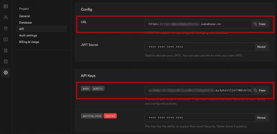
NEXT_PUBLIC_SUPABASE_URL=https://app-id.supabase.co NEXT_PUBLIC_SUPABASE_ANON_KEY=your-public-api-key
You can find the values of your API URL and API Key in the Supabase dashboard settings:
Next, create a file called api.js in the root of the project and add the following code:
// api.js import { createClient } from '@supabase/supabase-js' export const supabase = createClient( process.env.NEXT_PUBLIC_SUPABASE_URL, process.env.NEXT_PUBLIC_SUPABASE_ANON_KEY )
Now we will be able to import the supabase instance and use it anywhere in our app.
Here's an overview of what it looks like to interact with the API using the Supabase JavaScript client.
Querying for data:
import { supabase } from '../path/to/api' const { data, error } = await supabase .from('posts') .select()
Creating new items in the database:
const { data, error } = await supabase .from('posts') .insert([ { title: "Hello World", content: "My first post", user_id: "some-user-id", user_email: "[email protected]" } ])
As I mentioned earlier, the filters and modifiers make it really easy to implement various data access patterns and selection sets of your data.
Authentication – signing up:
const { user, session, error } = await supabase.auth.signUp({ email: '[email protected]', password: 'example-password', })
Authentication – signing in:
const { user, session, error } = await supabase.auth.signIn({ email: '[email protected]', password: 'example-password', })
In our case we won't be writing the main authentication logic by hand, we'll be using the Auth component from Supabase UI.
How to Build the App
Now let's start building out the UI!
To get started, let's first update the app to implement some basic navigation and layout styling.
We will also configure some logic to check if the user is signed in, and show a link for creating new posts if they are.
Finally we'll implement a listener for any auth events. And when a new auth event occurs, we'll check to make sure there is currently a signed in user in order to show or hide the Create Post link.
Open _app.js and add the following code:
// pages/_app.js import Link from 'next/link' import { useState, useEffect } from 'react' import { supabase } from '../api' import '../styles/globals.css' function MyApp({ Component, pageProps }) { const [user, setUser] = useState(null); useEffect(() => { const { data: authListener } = supabase.auth.onAuthStateChange( async () => checkUser() ) checkUser() return () => { authListener?.unsubscribe() }; }, []) async function checkUser() { const user = supabase.auth.user() setUser(user) } return ( <div> <nav className="p-6 border-b border-gray-300"> <Link href="/"> <span className="mr-6 cursor-pointer">Home</span> </Link> { user && ( <Link href="/create-post"> <span className="mr-6 cursor-pointer">Create Post</span> </Link> ) } <Link href="/profile"> <span className="mr-6 cursor-pointer">Profile</span> </Link> </nav> <div className="py-8 px-16"> <Component {...pageProps} /> </div> </div> ) } export default MyApp
How to make a user profile page
Next, let's create the profile page. In the pages directory, create a new file named profile.js and add the following code:
// pages/profile.js import { Auth, Typography, Button } from "@supabase/ui"; const { Text } = Typography import { supabase } from '../api' function Profile(props) { const { user } = Auth.useUser(); if (user) return ( <> <Text>Signed in: {user.email}</Text> <Button block onClick={() => props.supabaseClient.auth.signOut()}> Sign out </Button> </> ); return props.children } export default function AuthProfile() { return ( <Auth.UserContextProvider supabaseClient={supabase}> <Profile supabaseClient={supabase}> <Auth supabaseClient={supabase} /> </Profile> </Auth.UserContextProvider> ) }
The profile page uses the Auth component from the Supabase UI library. This component will render a "sign up" and "sign in" form for unauthenticated users, and a basic user profile with a "sign out" button for authenticated users. It will also enable a magic sign in link.
How to create new posts
Next, let's create the create-post page. In the pages directory, create a page named create-post.js with the following code:
// pages/create-post.js import { useState } from 'react' import { v4 as uuid } from 'uuid' import { useRouter } from 'next/router' import dynamic from 'next/dynamic' import "easymde/dist/easymde.min.css" import { supabase } from '../api' const SimpleMDE = dynamic(() => import('react-simplemde-editor'), { ssr: false }) const initialState = { title: '', content: '' } function CreatePost() { const [post, setPost] = useState(initialState) const { title, content } = post const router = useRouter() function onChange(e) { setPost(() => ({ ...post, [e.target.name]: e.target.value })) } async function createNewPost() { if (!title || !content) return const user = supabase.auth.user() const id = uuid() post.id = id const { data } = await supabase .from('posts') .insert([ { title, content, user_id: user.id, user_email: user.email } ]) .single() router.push(`/posts/${data.id}`) } return ( <div> <h1 className="text-3xl font-semibold tracking-wide mt-6">Create new post</h1> <input onChange={onChange} name="title" placeholder="Title" value={post.title} className="border-b pb-2 text-lg my-4 focus:outline-none w-full font-light text-gray-500 placeholder-gray-500 y-2" /> <SimpleMDE value={post.content} onChange={value => setPost({ ...post, content: value })} /> <button type="button" className="mb-4 bg-green-600 text-white font-semibold px-8 py-2 rounded-lg" onClick={createNewPost} >Create Post</button> </div> ) } export default CreatePost
This component renders a Markdown editor, allowing users to create new posts.
The createNewPost function will use the supabase instance to create new posts using the local form state.
You may notice that we are not passing in any headers. This is because if a user is signed in, the Supabase client libraries automatically include the access token in the headers for a signed in user.
How to view a single post
We need to configure a page to view a single post.
This page uses getStaticPaths to dynamically create pages at build time based on the posts coming back from the API.
We also use the fallback flag to enable fallback routes for dynamic SSG page generation.
We use getStaticProps to enable the Post data to be fetched and then passed into the page as props at build time.
Create a new folder in the pages directory called posts and a file called [id].js within that folder. In pages/posts/[id].js, add the following code:
// pages/posts/[id].js import { useRouter } from 'next/router' import ReactMarkdown from 'react-markdown' import { supabase } from '../../api' export default function Post({ post }) { const router = useRouter() if (router.isFallback) { return <div>Loading...</div> } return ( <div> <h1 className="text-5xl mt-4 font-semibold tracking-wide">{post.title}</h1> <p className="text-sm font-light my-4">by {post.user_email}</p> <div className="mt-8"> <ReactMarkdown className='prose' children={post.content} /> </div> </div> ) } export async function getStaticPaths() { const { data, error } = await supabase .from('posts') .select('id') const paths = data.map(post => ({ params: { id: JSON.stringify(post.id) }})) return { paths, fallback: true } } export async function getStaticProps ({ params }) { const { id } = params const { data } = await supabase .from('posts') .select() .filter('id', 'eq', id) .single() return { props: { post: data } } }
How to query for and render the list of posts
Next, let's update index.js to fetch and render a list of posts:
// pages/index.js import { useState, useEffect } from 'react' import Link from 'next/link' import { supabase } from '../api' export default function Home() { const [posts, setPosts] = useState([]) const [loading, setLoading] = useState(true) useEffect(() => { fetchPosts() }, []) async function fetchPosts() { const { data, error } = await supabase .from('posts') .select() setPosts(data) setLoading(false) } if (loading) return <p className="text-2xl">Loading ...</p> if (!posts.length) return <p className="text-2xl">No posts.</p> return ( <div> <h1 className="text-3xl font-semibold tracking-wide mt-6 mb-2">Posts</h1> { posts.map(post => ( <Link key={post.id} href={`/posts/${post.id}`}> <div className="cursor-pointer border-b border-gray-300 mt-8 pb-4"> <h2 className="text-xl font-semibold">{post.title}</h2> <p className="text-gray-500 mt-2">Author: {post.user_email}</p> </div> </Link>) ) } </div> ) }
Let's test it out
We now have all of the pieces of our app ready to go, so let's try it out.
To run the local server, run the dev command from your terminal:
npm run dev
When the app loads, you should see the following screen:

To sign up, click on Profile and create a new account. You should receive an email link to confirm your account after signing up.
You can also create a new account by using the magic link.
Once you're signed in, you should be able to create new posts:

Navigating back to the home page, you should be able to see a list of the posts that you've created and be able to click on a link to the post to view it:

How to Edit Posts
Now that we have the app up and running, let's learn how to edit posts. To get started with this, let's create a new view that will fetch only the posts that the signed in user has created.
To do so, create a new file named my-posts.js in the root of the project with the following code:
// pages/my-posts.js import { useState, useEffect } from 'react' import Link from 'next/link' import { supabase } from '../api' export default function MyPosts() { const [posts, setPosts] = useState([]) useEffect(() => { fetchPosts() }, []) async function fetchPosts() { const user = supabase.auth.user() const { data } = await supabase .from('posts') .select('*') .filter('user_id', 'eq', user.id) setPosts(data) } async function deletePost(id) { await supabase .from('posts') .delete() .match({ id }) fetchPosts() } return ( <div> <h1 className="text-3xl font-semibold tracking-wide mt-6 mb-2">My Posts</h1> { posts.map((post, index) => ( <div key={index} className="border-b border-gray-300 mt-8 pb-4"> <h2 className="text-xl font-semibold">{post.title}</h2> <p className="text-gray-500 mt-2 mb-2">Author: {post.user_email}</p> <Link href={`/edit-post/${post.id}`}><a className="text-sm mr-4 text-blue-500">Edit Post</a></Link> <Link href={`/posts/${post.id}`}><a className="text-sm mr-4 text-blue-500">View Post</a></Link> <button className="text-sm mr-4 text-red-500" onClick={() => deletePost(post.id)} >Delete Post</button> </div> )) } </div> ) }
In the query for the posts, we use the user id to select only the posts created by the signed in user.
Next, create a new folder named edit-post in the pages directory. Then, create a file named [id].js in this folder.
In this file, we'll be accessing the id of the post from a route parameter. When the component loads, we will then use the post id from the route to fetch the post data and make it available for editing.
In this file, add the following code:
// pages/edit-post/[id].js import { useEffect, useState } from 'react' import { useRouter } from 'next/router' import dynamic from 'next/dynamic' import "easymde/dist/easymde.min.css" import { supabase } from '../../api' const SimpleMDE = dynamic(() => import('react-simplemde-editor'), { ssr: false }) function EditPost() { const [post, setPost] = useState(null) const router = useRouter() const { id } = router.query useEffect(() => { fetchPost() async function fetchPost() { if (!id) return const { data } = await supabase .from('posts') .select() .filter('id', 'eq', id) .single() setPost(data) } }, [id]) if (!post) return null function onChange(e) { setPost(() => ({ ...post, [e.target.name]: e.target.value })) } const { title, content } = post async function updateCurrentPost() { if (!title || !content) return await supabase .from('posts') .update([ { title, content } ]) router.push('/my-posts') } return ( <div> <h1 className="text-3xl font-semibold tracking-wide mt-6 mb-2">Edit post</h1> <input onChange={onChange} name="title" placeholder="Title" value={post.title} className="border-b pb-2 text-lg my-4 focus:outline-none w-full font-light text-gray-500 placeholder-gray-500 y-2" /> <SimpleMDE value={post.content} onChange={value => setPost({ ...post, content: value })} /> <button className="mb-4 bg-blue-600 text-white font-semibold px-8 py-2 rounded-lg" onClick={updateCurrentPost}>Update Post</button> </div> ) } export default EditPost
Now, add a new link to our navigation located in pages/_app.js:
// pages/_app.js { user && ( <Link href="/my-posts"> <span className="mr-6 cursor-pointer">My Posts</span> </Link> ) }
When running the app, you should be able to view your own posts, edit them, and delete them from the updated UI.
How to enable real-time updates
Now that we have the app running it's trivial to add real-time updates.
By default, Realtime is disabled on your database. Let's turn on Realtime for the posts table.
To do so, open the app dashboard and click on Databases -> Replication -> 0 Tables (under Source). Toggle on Realtime functionality for the posts table. Here is a video walkthrough of how you can do this for clarity.
Next, open src/index.js and update the useEffect hook with the following code:
useEffect(() => { fetchPosts() const mySubscription = supabase .from('posts') .on('*', () => fetchPosts()) .subscribe() return () => supabase.removeSubscription(mySubscription) }, [])
Now, we will be subscribed to realtime changes in the posts table.
The code for the app is located here.
Next Steps
By now you should have a good understanding of how to build full stack apps with Supabase and Next.js.
If you'd like to learn more about building full stack apps with Supabase, I'd check out the following resources.
If you read this far, tweet to the author to show them you care.
0 notes
Text
Export and import data from Amazon S3 to Amazon Aurora PostgreSQL
You can build highly distributed applications using a multitude of purpose-built databases by decoupling complex applications into smaller pieces, which allows you to choose the right database for the right job. Amazon Aurora is the preferred choice for OLTP workloads. Aurora makes it easy to set up, operate, and scale a relational database in the cloud. This post demonstrates how you can export and import data from Amazon Aurora PostgreSQL-Compatible Edition to Amazon Simple Storage Service (Amazon S3) and shares associated best practices. The feature to export and import data to Amazon S3 is also available for Amazon Aurora MySQL-Compatible Edition. Overview of Aurora PostgreSQL-Compatible and Amazon S3 Aurora is a MySQL-compatible and PostgreSQL-compatible relational database built for the cloud. It combines the performance and availability of traditional enterprise databases with the simplicity and cost-effectiveness of open-source databases. Amazon S3 is an object storage service that offers industry-leading scalability, data availability, security, and performance. This means customers of all sizes and industries can use it to store and protect any amount of data. The following diagram illustrates the solution architecture. Prerequisites Before you get started, complete the following prerequisite steps: Launch an Aurora PostgreSQL DB cluster. You can also use an existing cluster. Note: To export data to Amazon S3 from Aurora PostgreSQL, your database must be running one of the following PostgreSQL engine versions 10.14 or higher, 11.9 or higher ,12.4 or higher Launch an Amazon EC2 instance that you installed the PostgreSQL client on. You can also use the pgAdmin tool or tool of your choice for this purpose. Create the required Identity and Access Management (IAM) policies and roles: Create an IAM policy with the least-restricted privilege to the resources in the following code and name it aurora-s3-access-pol. The policy must have access to the S3 bucket where the files are stored (for this post, aurora-pg-sample-loaddata01). { "Version": "2012-10-17", "Statement": [ { "Effect": "Allow", "Action": [ "s3:GetObject", "s3:AbortMultipartUpload", "s3:DeleteObject", "s3:ListMultipartUploadParts", "s3:PutObject", "s3:ListBucket" ], "Resource": [ "arn:aws:s3:::aurora-pg-sample-loaddata01/*", "arn:aws:s3:::aurora-pg-sample-loaddata01" ] } ] } Create two IAM roles named aurora-s3-export-role and aurora-s3-import-role and modify the trust relationships according to the following code. AssumeRole allows Aurora to access other AWS services on your behalf. {"Version": "2012-10-17","Statement": [ { "Effect": "Allow","Principal": { "Service": "rds.amazonaws.com" },"Action": "sts:AssumeRole" } ] } Attach the policy aurora-s3-access-pol from the previous step. For this post, we create the roles aurora-s3-export-role and aurora-s3-import-role. Their associated ARNs are arn:aws:iam::123456789012:role/aurora-s3-export-role and arn:aws:iam::123456789012:role/aurora-s3-import-role, respectively. Associate the IAM roles to the cluster. This enables the Aurora DB cluster to access the S3 bucket. See the following code: aws rds add-role-to-db-cluster --db-cluster-identifier aurora-postgres-cl --feature-name s3Export --role-arn arn:aws:iam::123456789012:role/aurora-s3-export-role aws rds add-role-to-db-cluster --db-cluster-identifier aurora-postgres-cl --feature-name s3Import --role-arn arn:aws:iam::123456789012:role/aurora-s3-import-role You’re now ready to explore the following use cases of exporting and importing data. Export data from Aurora PostgreSQL to Amazon S3 To export your data, complete the following steps: Connect to the cluster as the primary user, postgres in our case.By default, the primary user has permission to export and import data from Amazon S3. For this post, you create a test user with the least-required permission to export data to the S3 bucket. See the following code: psql -h aurora-postgres-cl.cluster-XXXXXXXXXXXX.us-east-1.rds.amazonaws.com -p 5432 -d pg1 -U postgres Install the required PostgreSQL extensions, aws_s3 and aws_commons. When you install the aws_s3 extension, the aws_commons extension is also installed: CREATE EXTENSION IF NOT EXISTS aws_s3 CASCADE; Create the user testuser (or you can use an existing user): create user testuser; password testuser; You can verify the user has been created with the du command: du testuser List of roles Role name | Attributes | Member of -----------+------------+----------- testuser | | {} Grant privileges on the aws_s3 schema to testuser (or another user you chose): grant execute on all functions in schema aws_s3 to testuser; Log in to the cluster as testuser: psql -h aurora-postgres-cl.cluster-XXXXXXXXXXXX.us-east-1.rds.amazonaws.com -p 5432 -d pg1 -U testuser Create and populate a test table called apg2s3_table, which you use for exporting data to the S3 bucket. You can use any existing table in your database (preferably small size) to test this feature. See the following code: CREATE TABLE apg2s3_table ( bid bigint PRIMARY KEY, name varchar(80) ); Insert a few records using the following statement: INSERT INTO apg2s3_table (bid,name) VALUES (1, 'Monday'), (2,'Tuesday'), (3, 'Wednesday'); To export data from the Aurora table to the S3 bucket, use the aws_s3.query_export_to_s3 and aws_commons.create_s3_uri functions: We use the aws_commons.create_s3_uri function to load a variable with the appropriate URI information required by the aws_s3.query_export_to_s3 function. The parameters required by the aws_commons.create_s3_uri function are the S3 bucket name, the full path (folder and filename) for the file to be created by the export command, and the Region. See the following example code: SELECT aws_commons.create_s3_uri( 'aurora-pg-sample-loaddata01', 'apg2s3_table', 'us-east-1' ) AS s3_uri_1 gset Export the entire table to the S3 bucket with the following code: SELECT * FROM aws_s3.query_export_to_s3( 'SELECT * FROM apg2s3_table',:'s3_uri_1'); rows_uploaded | files_uploaded | bytes_uploaded ---------------+----------------+---------------- 3 | 1 | 31 (1 row) If you’re trying this feature out for the first time, consider using the LIMIT clause for a larger table. If you’re using a PostgreSQL client that doesn’t have the gset command available, the workaround is to call the aws_commons.create_s3_uri function inside of the aws_s3.query_export_to_s3 function as follows: SELECT * FROM aws_s3.query_export_to_s3( 'SELECT * FROM apg2s3_table', aws_commons.create_s3_uri( 'aurora-pg-sample-loaddata01', 'apg2s3_table','us-east-1')); rows_uploaded | files_uploaded | bytes_uploaded ---------------+----------------+---------------- 3 | 1 | 31 (1 row) The final step is to verify the export file was created in the S3 bucket. The default file size threshold is 6 GB. Because the data selected by the statement is less than the file size threshold, a single file is created: aws s3 ls s3://aurora-pg-sample-loaddata01/apg2s3_table --human-readable --summarize 2020-12-12 12:06:59 31 Bytes apg2s3_table Total Objects: 1 Total Size: 31 Bytes If you need the file size to be smaller than 6 GB, you can identify a column to split the table data into small portions and run multiple SELECT INTO OUTFILE statements (using the WHERE condition). It’s best to do this when the amount of data selected is more than 25 GB. Import data from Amazon S3 to Aurora PostgreSQL In this section, you load the data back to the Aurora table from the S3 file. Complete the following steps: Create a new table called apg2s3_table_imp: CREATE TABLE apg2s3_table_imp( bid bigint PRIMARY KEY, name varchar(80) ); Use the create_s3_uri function to load a variable named s3_uri_1 with the appropriate URI information required by the aws_s3.table_import_from_s3 function: SELECT aws_commons.create_s3_uri( 'aurora-pg-sample-loaddata01', 'apg2s3_table','us-east-1') AS s3_uri_1 gset Use the aws_s3.table_import_from_s3 function to import the data file from an Amazon S3 prefix: SELECT aws_s3.table_import_from_s3( 'apg2s3_table_imp', '', '(format text)', :'s3_uri_1' ); Verify the information was loaded into the apg2s3_table_imp table: SELECT * FROM apg2s3_table_imp; Best practices This section discusses a few best practices for bulk loading large datasets from Amazon S3 to your Aurora PostgreSQL database. The observations we present are based on a series of tests loading 100 million records to the apg2s3_table_imp table on a db.r5.2xlarge instance (see the preceding sections for table structure and example records). We carried out load testing when no other active transactions were running on the cluster. Results might vary depending on your cluster loads and instance type. The baseline load included 100 million records using the single file apg2s3_table.csv, without any structural changes to the target table apg2s3_table_imp or configuration changes to the Aurora PostgreSQL database. The data load took approximately 360 seconds. See the following code: time psql -h aurora-postgres-cl.cluster-XXXXXXXXXXXX.us-east-1.rds.amazonaws.com -p 5432 -U testuser -d pg1 -c "SELECT aws_s3.table_import_from_s3('apg2s3_table_imp','','(format CSV)','aurora-pg-sample-loaddata01','apg2s3_table.csv','us-east-1')" table_import_from_s3 --------------------------------------------------------------------------------------------------------- 100000000 rows imported into relation "apg2s3_table_imp" from file apg2s3_table.csv of 3177777796 bytes (1 row) real 6m0.368s user 0m0.005s sys 0m0.005s We used the same dataset to implement some best practices iteratively to measure their performance benefits on the load times. The following best practices are listed in order of the observed performance benefits from lower to higher improvements. Drop indexes and constraints Although indexes can significantly increase the performance of some DML operations such as UPDATE and DELETE, these data structures can also decrease the performance of inserts, especially when dealing with bulk data inserts. The reason is that after each new record is inserted in the table, the associated indexes also need to be updated to reflect the new rows being loaded. Therefore, a best practice for bulk data loads is dropping indexes and constraints on the target tables before a load and recreating them when the load is complete. In our test case, by dropping the primary key and index associated with the apg2s3_table_imp table, we reduced the data load down to approximately 131 seconds (data load + recreation on primary key). This is roughly 2.7 times faster than the baseline. See the following code: psql -h aurora-postgres-cl.cluster-XXXXXXXXXXXX.us-east-1.rds.amazonaws.com -p 5432 -U testuser -d pg1 -c "d apg2s3_table_imp" Table "public.apg2s3_table_imp" Column | Type | Collation | Nullable | Default | Storage | Stats target | Description --------+-----------------------+-----------+----------+---------+----------+--------------+------------- bid | bigint | | not null | | plain | | name | character varying(80) | | | | extended | | Indexes: "apg2s3_table_imp_pkey" PRIMARY KEY, btree (bid) psql -h aurora-postgres-cl.cluster-XXXXXXXXXXXX.us-east-1.rds.amazonaws.com -p 5432 -U testuser -d pg1 -c "ALTER TABLE apg2s3_table_imp DROP CONSTRAINT apg2s3_table_imp_pkey" ALTER TABLE psql -h aurora-postgres-cl.cluster-XXXXXXXXXXXX.us-east-1.rds.amazonaws.com -p 5432 -U testuser -d pg1 -c "d apg2s3_table_imp" Table "public.apg2s3_table_imp" Column | Type | Collation | Nullable | Default --------+-----------------------+-----------+----------+--------- bid | bigint | | not null | name | character varying(80) | | | time psql -h aurora-postgres-cl.cluster-XXXXXXXXXXXX.us-east-1.rds.amazonaws.com -p 5432 -U testuser -d pg1 -c "SELECT aws_s3.table_import_from_s3('apg2s3_table_imp','','(format CSV)','aurora-pg-sample-loaddata01','apg2s3_table.csv','us-east-1')" table_import_from_s3 --------------------------------------------------------------------------------------------------------- 100000000 rows imported into relation "apg2s3_table_imp" from file apg2s3_table.csv of 3177777796 bytes (1 row) real 1m24.950s user 0m0.005s sys 0m0.005s time psql -h demopg-instance-1.cmcmpwi7rtng.us-east-1.rds.amazonaws.com -p 5432 -U testuser -d pg1 -c "ALTER TABLE apg2s3_table_imp ADD PRIMARY KEY (bid);" ALTER TABLE real 0m46.731s user 0m0.009s sys 0m0.000s Concurrent loads To improve load performance, you can split large datasets into multiple files that can be loaded concurrently. However, the degree of concurrency can impact other transactions running on the cluster. The number of vCPUs allocated to instance types plays a key role because load operation requires CPU cycles to read data, insert into tables, commit changes, and more. For more information, see Amazon RDS Instance Types. Loading several tables concurrently with few vCPUs can cause CPU utilization to spike and may impact the existing workload. For more information, see Overview of monitoring Amazon RDS. For our test case, we split the original file into five pieces of 20 million records each. Then we created simple shell script to run a psql command for each file to be loaded, like the following: #To make the test simpler, we named the datafiles as apg2s3_table_imp_XX. #Where XX is a numeric value between 01 and 05 for i in 1 2 3 4 5 do myFile=apg2s3_table_imp_0$i psql -h aurora-postgres-cl.cluster-cmcmpwi7rtng.us-east-1.rds.amazonaws.com -p 5432 -U testuser -d pg1 -c "SELECT aws_s3.table_import_from_s3( 'apg2s3_table_imp', '', '(format CSV)','aurora-pg-sample-loaddata01','$myFile','us-east-1')" & done wait You can export the PGPASSWORD environment variable in the session where you’re running the script to prevent psql from prompting for a database password. Next, we ran the script: time ./s3Load5 table_import_from_s3 ---------------------------------------------------------------------------------------------------------- 20000000 rows imported into relation "apg2s3_table_imp" from file apg2s3_table_imp_01 of 617777794 bytes (1 row) table_import_from_s3 ---------------------------------------------------------------------------------------------------------- 20000000 rows imported into relation "apg2s3_table_imp" from file apg2s3_table_imp_02 of 640000000 bytes (1 row) table_import_from_s3 ---------------------------------------------------------------------------------------------------------- 20000000 rows imported into relation "apg2s3_table_imp" from file apg2s3_table_imp_03 of 640000002 bytes (1 row) table_import_from_s3 ---------------------------------------------------------------------------------------------------------- 20000000 rows imported into relation "apg2s3_table_imp" from file apg2s3_table_imp_04 of 640000000 bytes (1 row) table_import_from_s3 ---------------------------------------------------------------------------------------------------------- 20000000 rows imported into relation "apg2s3_table_imp" from file apg2s3_table_imp_05 of 640000000 bytes (1 row) real 0m40.126s user 0m0.025s sys 0m0.020s time psql -h demopg-instance-1.cmcmpwi7rtng.us-east-1.rds.amazonaws.com -p 5432 -U testuser -d pg1 -c "ALTER TABLE apg2s3_table_imp ADD PRIMARY KEY (bid);" ALTER TABLE real 0m48.087s user 0m0.006s sys 0m0.003s The full load duration, including primary key rebuild, was reduced to approximately 88 seconds, which demonstrates the performance benefits of parallel loads. Implement partitioning If you’re using partitioned tables, consider loading partitions in parallel to further improve load performance. To test this best practice, we partition the apg2s3_table_imp table on the bid column as follows: CREATE TABLE apg2s3_table_imp ( bid BIGINT, name VARCHAR(80) ) PARTITION BY RANGE(bid); CREATE TABLE apg2s3_table_imp_01 PARTITION OF apg2s3_table_imp FOR VALUES FROM (1) TO (20000001); CREATE TABLE apg2s3_table_imp_02 PARTITION OF apg2s3_table_imp FOR VALUES FROM (20000001) TO (40000001); CREATE TABLE apg2s3_table_imp_03 PARTITION OF apg2s3_table_imp FOR VALUES FROM (40000001) TO (60000001); CREATE TABLE apg2s3_table_imp_04 PARTITION OF apg2s3_table_imp FOR VALUES FROM (60000001) TO (80000001); CREATE TABLE apg2s3_table_imp_05 PARTITION OF apg2s3_table_imp FOR VALUES FROM (80000001) TO (MAXVALUE); To load all the partitions in parallel, we modified the shell script used in the previous example: #To make the test simpler, we named the datafiles as apg2s3_table_imp_XX. #Where XX is a numeric value between 01 and 05 for i in 1 2 3 4 5 do myFile=apg2s3_table_imp_0$i psql -h aurora-postgres-cl.cluster-cmcmpwi7rtng.us-east-1.rds.amazonaws.com -p 5432 -U testuser -d pg1 -c "SELECT aws_s3.table_import_from_s3( '$myFile', '', '(format CSV)','aurora-pg-sample-loaddata01','$myFile','us-east-1')" & done wait Then we ran the script to load all five partitions in parallel: time ./s3LoadPart table_import_from_s3 ------------------------------------------------------------------------------------------------------------- 20000000 rows imported into relation "apg2s3_table_imp_04" from file apg2s3_table_imp_04 of 640000000 bytes (1 row) table_import_from_s3 ------------------------------------------------------------------------------------------------------------- 20000000 rows imported into relation "apg2s3_table_imp_02" from file apg2s3_table_imp_02 of 640000000 bytes (1 row) table_import_from_s3 ------------------------------------------------------------------------------------------------------------- 20000000 rows imported into relation "apg2s3_table_imp_05" from file apg2s3_table_imp_05 of 640000002 bytes (1 row) table_import_from_s3 ------------------------------------------------------------------------------------------------------------- 20000000 rows imported into relation "apg2s3_table_imp_01" from file apg2s3_table_imp_01 of 617777794 bytes (1 row) table_import_from_s3 ------------------------------------------------------------------------------------------------------------- 20000000 rows imported into relation "apg2s3_table_imp_03" from file apg2s3_table_imp_03 of 640000000 bytes (1 row) real 0m28.665s user 0m0.022s sys 0m0.024s $ time psql -h demopg-instance-1.cmcmpwi7rtng.us-east-1.rds.amazonaws.com -p 5432 -U testuser -d pg1 -c "ALTER TABLE apg2s3_table_imp ADD PRIMARY KEY (bid);" ALTER TABLE real 0m48.516s user 0m0.005s sys 0m0.004s Loading all partitions concurrently reduced the load times even further, to approximately 77 seconds. Disable triggers Triggers are frequently used in applications to perform additional processing after certain conditions (such as INSERT, UPDATE, or DELETE DML operations) run against tables. Because of this additional processing, performing large data loads on a table where triggers are enabled can decrease the load performance substantially. It’s recommended to disable triggers prior to bulk load operations and re-enable them when the load is complete. Summary This post demonstrated how to import and export data between Aurora PostgreSQL and Amazon S3. Aurora is powered with operational analytics capabilities, and integration with Amazon S3 makes it easier to establish an agile analytical environment. For more information about importing and exporting data, see Migrating data to Amazon Aurora with PostgreSQL compatibility. For more information about Aurora best practices, see Best Practices with Amazon Aurora PostgreSQL. About the authors Suresh Patnam is a Solutions Architect at AWS. He helps customers innovate on the AWS platform by building highly available, scalable, and secure architectures on Big Data and AI/ML. In his spare time, Suresh enjoys playing tennis and spending time with his family. Israel Oros is a Database Migration Consultant at AWS. He works with customers in their journey to the cloud with a focus on complex database migration programs. In his spare time, Israel enjoys traveling to new places with his wife and riding his bicycle whenever weather permits. https://aws.amazon.com/blogs/database/export-and-import-data-from-amazon-s3-to-amazon-aurora-postgresql/
0 notes
Text
Many To One(Uni-directional) Relational Mapping with Spring Boot + Spring Data JPA + H2 Database
In this tutorial , we will see Many To One mapping of two entities using Spring Boot and Spring Data JPA using H2 database. GitHub Link – Download Tools: Spring BootSpring Data JPAH2 DatabaseIntelliJ IDEAMaven We have two entities Student and Department. Many students are part of one Department (Many To One). This is called Many To One mapping between two entities. For each of this entity, table will be created in database. So there will be two tables created in database. create table address (id bigint generated by default as identity, name varchar(255), primary key (id)); create table student (id bigint generated by default as identity, mobile integer, name varchar(255), address_id bigint, primary key (id)); alter table student add constraint FKcaf6ht0hfw93lwc13ny0sdmvo foreign key (address_id) references address(id); Each table has primary key as ID . Two tables has Many To One relationship between them as each department has many students in them. STUDENT table has foreign key as DEPT_ID in it. So STUDENT is a child table and DEPARTMENT table is parent table in this relationship. FOREIGN KEY constraint adds below restrictions - We can't add records in child table if there is no entry in parent table. Ex. You can't add department ID reference in STUDENT table if department ID is not present in DEPARTMENT table.You can't delete the records from parent table unless corresponding references are deleted from child table . Ex. You can't delete the entry DEPARTMENT table unless corresponding students from STUDENT table are deleted . You can apply ON_DELETE_CASCADE with foreign key constraint if you want to delete students from STUDENT table automatically when department is deleted. If you want to insert a student into STUDENT table then corresponding department should already be present in DEPARTMENT table.When any department is updated in DEPARTMENT table then child table will also see the updated reference from parent table Now we will see how can we form this relationship using Spring data JPA entities. Step 1: Define all the dependencies required for this project 4.0.0 org.springframework.boot spring-boot-starter-parent 2.1.1.RELEASE com.myjavablog springboot-jpa-one-to-many-demo 0.0.1-SNAPSHOT springboot-jpa-one-to-many-demo Demo project for Spring Boot 1.8 org.springframework.boot spring-boot-starter org.springframework.boot spring-boot-starter-test test org.springframework.boot spring-boot-starter-web org.springframework.boot spring-boot-starter-tomcat org.springframework.boot spring-boot-starter-data-jpa org.apache.tomcat tomcat-jdbc com.h2database h2 org.springframework.boot spring-boot-starter-test test colt colt 1.2.0 org.springframework.boot spring-boot-maven-plugin spring-boot-starter-data-jpa – This jar is used to connect to database .It also has a support to provide different JPA implementations to interact with the database like Hibernate, JPA Repository, CRUD Repository etc. h2 – Its used to create H2 database when the spring boot application boots up. Spring boot will read the database configuration from application.properties file and creates a DataSource out of it. Step 2: Define the Model/Entity classes Student.java package com.myjavablog.model; import org.springframework.stereotype.Repository; import javax.annotation.Generated; import javax.persistence.*; import java.util.Optional; @Entity @Table(name = "STUDENT") public class Student { @Id @GeneratedValue(strategy = GenerationType.IDENTITY) private Long id; @Column private String name; @Column private int mobile; @ManyToOne(cascade = CascadeType.ALL) @JoinColumn(name = "DEPT_ID") private Department department; public Long getId() { return id; } public void setId(Long id) { this.id = id; } public String getName() { return name; } public void setName(String name) { this.name = name; } public int getMobile() { return mobile; } public void setMobile(int mobile) { this.mobile = mobile; } public Department getDepartment() { return department; } public void setDepartment(Department department) { this.department = department; } } Department.java package com.myjavablog.model; import javax.persistence.*; import java.util.List; @Entity @Table(name = "DEPARTMENT") public class Department { @Id @GeneratedValue(strategy = GenerationType.IDENTITY) private Long id; @Column private String name; public Long getId() { return id; } public void setId(Long id) { this.id = id; } public String getName() { return name; } public void setName(String name) { this.name = name; } } Below are the Annotations used while creating the entity classes - Spring Data JPA Annotations - @Entity - This annotation marks the class annotations.@Table - This annotation creates table in database.@Id - It creates primary key in table.@GeneratedValue - It defines primary key generation strategy like AUTO,IDENTITY,SEQUENCE etc.@Column - It defines column property for table.@ManyToOne - This annotation creates Many to One relationship between Student and Department entities. The cascade property (CascadeType.ALL) defines what should happen with child table records when something happens with parent table records. On DELETE, UPDATE , INSERT operations in parent table child table should also be affected. Only @ManyToOne annotation is enough to form one-to-many relationaship. This annotation is generally used in child entity to form Unidirectional relational mapping.@JoinColumn - You can define column which creates foreign key in a table. In our example, DEPT_ID is a foreign key in STUDENT table which references to ID in DEPARTMENT table. Step 3: Create the JPA repositories to query STUDENT and DEPARTMENT tables StudentRepository and AddressRepository implemets JpaRepository which has methods to perform all CRUD operations. It has methods like save(), find(), delete(),exists(),count() to perform database operations. package com.myjavablog.dao; import com.myjavablog.model.Student; import org.springframework.data.jpa.repository.JpaRepository; import org.springframework.stereotype.Repository; @Repository public interface StudentRepository extends JpaRepository { public Student findByName(String name); } package com.myjavablog.dao; import com.myjavablog.model.Address; import org.springframework.data.jpa.repository.JpaRepository; import org.springframework.stereotype.Repository; @Repository public interface AddressRepository extends JpaRepository{ } Step 4: Create the class BeanConfig to configure the bean for H2 database This class creates a bean ServletRegistrationBean and autowires it to spring container. This bean actually required to access H2 database from console through browser. package com.myjavablog; import org.h2.server.web.WebServlet; import org.springframework.boot.web.servlet.ServletRegistrationBean; import org.springframework.context.annotation.Bean; import org.springframework.context.annotation.Configuration; @Configuration public class BeanConfig { @Bean ServletRegistrationBean h2servletRegistration() { ServletRegistrationBean registrationBean = new ServletRegistrationBean(new WebServlet()); registrationBean.addUrlMappings("/console/*"); return registrationBean; } } Step 5: Last but not the least, You need to define application properties. #DATASOURCE (DataSourceAutoConfiguration & #DataSourceProperties) spring.datasource.url=jdbc:h2:mem:testdb;DB_CLOSE_ON_EXIT=FALSE spring.datasource.username=sa spring.datasource.password= #Hibernate #The SQL dialect makes Hibernate generate better SQL for the chosen #database spring.jpa.properties.hibernate.dialect =org.hibernate.dialect.H2Dialect spring.datasource.driverClassName=org.h2.Driver #Hibernate ddl auto (create, create-drop, validate, update) spring.jpa.hibernate.ddl-auto = update logging.level.org.hibernate.SQL=DEBUG logging.level.org.hibernate.type=TRACE server.port=8082 server.error.whitelabel.enabled=false Step 6: Create the spring boot main file package com.myjavablog; import com.myjavablog.dao.DepartmentRepository; import com.myjavablog.dao.StudentRepository; import com.myjavablog.model.Department; import com.myjavablog.model.Student; import org.springframework.beans.factory.annotation.Autowired; import org.springframework.boot.CommandLineRunner; import org.springframework.boot.SpringApplication; import org.springframework.boot.autoconfigure.SpringBootApplication; import org.springframework.data.jpa.repository.config.EnableJpaRepositories; import java.util.Arrays; @SpringBootApplication public class SpringbootJpaOneToManyDemoApplication implements CommandLineRunner { @Autowired private DepartmentRepository departmentRepository; @Autowired private StudentRepository studentRepository; public static void main(String args) { SpringApplication.run(SpringbootJpaOneToManyDemoApplication.class, args); } @Override public void run(String... args) throws Exception { //Unidirectional Mapping Department department = new Department(); department.setName("COMPUTER"); departmentRepository.save(department); Student student = new Student(); student.setDepartment(departmentRepository.findDepartmentByName("COMPUTER")); student.setName("Anup"); student.setMobile(989911); Student student1 = new Student(); student1.setDepartment(departmentRepository.findDepartmentByName("IT")); student1.setName("John"); student1.setMobile(89774); studentRepository.saveAll(Arrays.asList(student,student1)); } } Step 7: Now run the application Run the application as a java application or as spring boot application spring-boot:run Once you run the application records will be inserted to tables as below -

Step 8: This application also has REST endpoints to expose the services as below - Save department -

Add students under created department -

We can check database entries to cross verify -

Read the full article
0 notes
Text
Azure SQL Database vs Azure SQL Data Warehouse
Back in 2013, Microsoft introduced Azure SQL Database that has its origin in the on-premises Microsoft SQL Server. In 2015 (however public availability was in July 2016) Microsoft added SQL Data Warehouse to the Azure cloud portfolio that has its origin in the on-premises Microsoft Analytics Platform System (APS). This was a Parallel Data Warehouse (PDW) coupled with Massively Parallel Processing (MPP) technology and included standard hardware
The differences between those two Microsoft Azure Services, but first Microsoft own definitions:
Azure SQL Database is just a comparative database-as-a service using the Microsoft SQL Server Engine.
Azure SQL Data Warehouse is just a massively parallel processing (MPP) cloud-based, scale-out, relational database capable of processing massive volumes of data.

Differences
1) Purpose: OLAP vs OLTP
Although both Azure SQL DB and Azure SQL DW are cloud based systems for hosting data, their principle is different. The biggest difference is that SQL DB is especially for Online Transaction Processing (OLTP). This means operational data with lots of short transactions like INSERT, UPDATE and DELETE by multiple people and/or processes. The info is usually highly normalized stored in many tables.
On another hand SQL DW is especially for Online Analytical Processing (OLAP) for data warehouses. This means consolidation data with a diminished volume, but more technical queries. The info is usually stored de-normalized with fewer tables utilizing a star or snowflake schema.
2) Architecture
In order to make the differences more clear a quick preview of the architecture of Azure SQL Data Warehouse, where you see an entire assortment of Azure SQL Databases and separated storage. The utmost number of compute notes at this time is 60.
3) Storage size
The present size limit of an Azure SQL Database is 4TB, but it has been getting bigger in the last couple of years and will likely find yourself around 10TB in the near future. On another hand we have the Azure SQL Data Warehouse which has no storage limit at all (only the limit of one's wallet), as the storage is separated from the compute.
4) Pricing
The pricing can also be quite different. Where Azure SQL DB starts with €4,20 a month, Azure SQL DW starts around €900,- a month excluding the expense of storage that will be included in SQL DB. The storage costs for Azure SQL DW remain €125, - per TB per month. And the maximum costs of just one SQL DB is around €13500, - where SQL DW ends around a huge €57000, - (excl. storage). But once you have a look at the architecture above, it should be no surprise that SQL DW is higher priced than SQL DB, because it consists of multiple SQL DBs.
5) Concurrent Connection
Although SQL DW is a collection of SQL Databases the maximum number of concurrent connections is significantly less than with SQL DB. SQL DW has a maximum of 1024 active connections where SQL DB are designed for 6400 concurrent logins and 30000 concurrent sessions. Which means in the exceptional case where you have over a thousand active users for your dashboard you most likely should consider SQL DB to host the info as opposed to SQL DW.
6) Concurrent Queries
Besides the maximum connections, the amount of concurrent queries can also be much lower. SQL DW can execute a maximum of 32 queries at one moment where SQL DB might have 6400 concurrent workers (requests). That is where you see the differences between OLTP and OLAP.
7) PolyBase
Azure SQL Data Warehouse supports PolyBase. This technology enables you to access data away from database with regular Transact SQL. It could for example use a file in an Azure Blob Storage container as a (external) table. Other options are importing and exporting data from Hadoop or Azure Data Lake Store. Although SQL Server 2016 also supports PolyBase, Azure SQL Database doesn't support it.
8) Query language differences
Although SQL DW uses SQL DB in the backdrop there are always a few minor differences when querying or creating tables:
· SQL DW cannot use cross databases queries. So all important computer data should maintain the exact same database.
· SQL DW can use IDENTITY, but just for INT or BIGINT. Moreover the IDENTITY column cannot be used within the distribution key.
9) Replication
SQL DB supports active geo-replication. This lets you configure up to four readable secondary databases in the exact same or different location. SQL DW doesn't support active geo-replication, only Azure Storage replication. However this is not really a live, readable, synchronized copy of one's database! It's more such as a backup.
10) In Memory OLTP tables
SQL DB supports in-memory OLTP. SQL DW is OLAP and doesn't support it.
11) Always encrypted
SQL DB supports Always Encrypted to guard sensitive data. SQL DW doesn't support it.
For more information CLICK HERE.
#MS Azure Online Training#Azure Online Training#Azure Training#Microsoft Azure Training in Hyderabad#MS Azure Training in Ameerpet#MS Azure Training in Hyderabad
0 notes
Text
VB.Net DAL Generator - Source Code (Database Abstractions)
VB.Net DAL Generator is a .net desktop application that generates VB.Net Data Access Layer for SQL Server and MS Access databases. The purpose of this application is to make software development easy. It creates VB.Net classes (one per table) that contain methods for CRUD operations. The generated code can be used in web as well as desktop apps.
If you need C# DAL Generator for SQL Server and MS Access then click here. If you need C# DAL Generator for MySQL then click here. If you need DAL Generator for Entity Framework (C#/VB.Net) then click here. If you need PHP Code Generator for MySQL/MySQLi/PDO then click here.
Video Demo:
Click here to view the video demo.
Features:
It creates VB.Net classes (one for each table).
Supports SQL Server and MS Access.
The class contains all columns of the table as properties.
Data types have been handled nicely.
Creates methods for CRUD operations.
Sorting has been handled.
Pagination has been handled (SQL Server only).
Primary key is automatically detected for each table.
Composite primary key is supported.
Nullable columns have been handled.
Identity column has been handled.
Timestamp column has been handled.
Completely indented code is generated.
The generated code can be used in both desktop and web applications.
All the following data types of SQL Server are supported: char, nchar, varchar, nvarchar, text, ntext, xml, decimal, numeric, money, smallmoney, bit, binary, image, timestamp, varbinary, date, datetime, datetime2, smalldatetime, datetimeoffset, time, bigint, int, smallint, tinyint, float, real, uniqueidentifier, sql_variant
Source code (written in C#) has also been provided so that to enable users to make changes according to their programming structure.
Sample Application:
A sample web application has also been provided that is using the generated code. In this application one form (for employees) has been created. This app uses the generated data access layer without modifying a single line in the generated code.
Generated Code:
VB.Net Class: For each table one VB.Net class is created that contains all columns of the table as properties.
Add Method: It is an instance method. It adds a new record to the relevant table. Nullable columns have been handled properly. If you don’t want to insert values in the nullable columns, don’t specify values for the relevant properties. Identity and timestamp columns cannot be inserted manually therefore these columns are skipped while inserting a record. Relevant property of the identity column is populated after record is inserted.
Update Method: It is an instance method. It updates an existing record. Identity and timestamp columns are skipped while updating a record.
Delete Method: It is a shared method. It deletes an existing record. It takes primary key columns values as parameters.
Get Method: It is a shared method. It gets an existing record (an instance of the class is created and all properties are populated). It takes primary key columns values as parameters.
GetAll Method: It is a shared method. It gets all records of the relevant table. You can also specify search columns. If sorting/pagination is enabled then the relevant code will also be generated.
from CodeCanyon new items http://ift.tt/2sSyjzP via IFTTT https://goo.gl/zxKHwc
0 notes
Text
Better Reducers With Immer
About The Author
Awesome frontend developer who loves everything coding. I’m a lover of choral music and I’m working to make it more accessible to the world, one upload at a … More about Chidi …
In this article, we’re going to learn how to use Immer to write reducers. When working with React, we maintain a lot of state. To make updates to our state, we need to write a lot of reducers. Manually writing reducers results in bloated code where we have to touch almost every part of our state. This is tedious and error-prone. In this article, we’re going to see how Immer brings more simplicity to the process of writing state reducers.
As a React developer, you should be already familiar with the principle that state should not be mutated directly. You might be wondering what that means (most of us had that confusion when we started out).
This tutorial will do justice to that: you will understand what immutable state is and the need for it. You’ll also learn how to use Immer to work with immutable state and the benefits of using it. You can find the code in this article in this Github repo.
Immutability In JavaScript And Why It Matters
Immer.js is a tiny JavaScript library was written by Michel Weststrate whose stated mission is to allow you “to work with immutable state in a more convenient way.”
But before diving into Immer, let’s quickly have a refresher about immutability in JavaScript and why it matters in a React application.
The latest ECMAScript (aka JavaScript) standard defines nine built-in data types. Of these nine types, there are six that are referred to as primitive values/types. These six primitives are undefined, number, string, boolean, bigint, and symbol. A simple check with JavaScript’s typeof operator will reveal the types of these data types.
console.log(typeof 5) // numberconsole.log(typeof 'name') // stringconsole.log(typeof (1
A primitive is a value that is not an object and has no methods. Most important to our present discussion is the fact that a primitive’s value cannot be changed once it is created. Thus, primitives are said to be immutable.
The remaining three types are null, object, and function. We can also check their types using the typeof operator.
console.log(typeof null) // objectconsole.log(typeof [0, 1]) // objectconsole.log(typeof {name: 'name'}) // objectconst f = () => ({})console.log(typeof f) // function
These types are mutable. This means that their values can be changed at any time after they are created.
You might be wondering why I have the array [0, 1] up there. Well, in JavaScriptland, an array is simply a special type of object. In case you’re also wondering about null and how it is different from undefined. undefined simply means that we haven’t set a value for a variable while null is a special case for objects. If you know something should be an object but the object is not there, you simply return null.
To illustrate with a simple example, try running the code below in your browser console.
console.log('aeiou'.match(/[x]/gi)) // nullconsole.log('xyzabc'.match(/[x]/gi)) // [ 'x' ]
String.prototype.match should return an array, which is an object type. When it can’t find such an object, it returns null. Returning undefined wouldn’t make sense here either.
Enough with that. Let’s return to discussing immutability.
According to the MDN docs:
“All types except objects define immutable values (that is, values which can’t be changed).”
This statement includes functions because they are a special type of JavaScript object. See function definition here.
Let’s take a quick look at what mutable and immutable data types mean in practice. Try running the below code in your browser console.
let a = 5;let b = aconsole.log(`a: ${a}; b: ${b}`) // a: 5; b: 5b = 7console.log(`a: ${a}; b: ${b}`) // a: 5; b: 7
Our results show that even though b is “derived” from a, changing the value of b doesn’t affect the value of a. This arises from the fact that when the JavaScript engine executes the statement b = a, it creates a new, separate memory location, puts 5 in there, and points b at that location.
What about objects? Consider the below code.
let c = { name: 'some name'}let d = c;console.log(`c: ${JSON.stringify(c)}; d: ${JSON.stringify(d)}`) // {"name":"some name"}; d: {"name":"some name"}d.name = 'new name'console.log(`c: ${JSON.stringify(c)}; d: ${JSON.stringify(d)}`) // {"name":"new name"}; d: {"name":"new name"}
We can see that changing the name property via variable d also changes it in c. This arises from the fact that when the JavaScript engine executes the statement, c = { name: 'some name' }, the JavaScript engine creates a space in memory, puts the object inside, and points c at it. Then, when it executes the statement d = c, the JavaScript engine just points d to the same location. It doesn’t create a new memory location. Thus any changes to the items in d is implicitly an operation on the items in c. Without much effort, we can see why this is trouble in the making.
Imagine you were developing a React application and somewhere you want to show the user’s name as some name by reading from variable c. But somewhere else you had introduced a bug in your code by manipulating the object d. This would result in the user’s name appearing as new name. If c and d were primitives we wouldn’t have that problem. But primitives are too simple for the kinds of state a typical React application has to maintain.
This is about the major reasons why it is important to maintain an immutable state in your application. I encourage you to check out a few other considerations by reading this short section from the Immutable.js README: the case for immutability.
Having understood why we need immutability in a React application, let’s now take a look at how Immer tackles the problem with its produce function.
Immer’s produce Function
Immer’s core API is very small, and the main function you’ll be working with is the produce function. produce simply takes an initial state and a callback that defines how the state should be mutated. The callback itself receives a draft (identical, but still a copy) copy of the state to which it makes all the intended update. Finally, it produces a new, immutable state with all the changes applied.
The general pattern for this sort of state update is:
// produce signatureproduce(state, callback) => nextState
Let’s see how this works in practice.
import produce from 'immer' const initState = { pets: ['dog', 'cat'], packages: [ { name: 'react', installed: true }, { name: 'redUX', installed: true }, ],} // to add a new packageconst newPackage = { name: 'immer', installed: false } const nextState = produce(initState, draft => { draft.packages.push(newPackage)})
In the above code, we simply pass the starting state and a callback that specifies how we want the mutations to happen. It’s as simple as that. We don’t need to touch any other part of the state. It leaves initState untouched and structurally shares those parts of the state that we didn’t touch between the starting and the new states. One such part in our state is the pets array. The produced nextState is an immutable state tree that has the changes we’ve made as well as the parts we didn’t modify.
Armed with this simple, but useful knowledge, let’s take a look at how produce can help us simplify our React reducers.
Writing Reducers With Immer
Suppose we have the state object defined below
const initState = { pets: ['dog', 'cat'], packages: [ { name: 'react', installed: true }, { name: 'redUX', installed: true }, ],};
And we wanted to add a new object, and on a subsequent step, set its installed key to true
const newPackage = { name: 'immer', installed: false };
If we were to do this the usual way with JavaScripts object and array spread syntax, our state reducer might look like below.
const updateReducer = (state = initState, action) => { switch (action.type) { case 'ADD_PACKAGE': return { ...state, packages: [...state.packages, action.package], }; case 'UPDATE_INSTALLED': return { ...state, packages: state.packages.map(pack => pack.name === action.name ? { ...pack, installed: action.installed } : pack ), }; default: return state; }};
We can see that this is unnecessarily verbose and prone to mistakes for this relatively simple state object. We also have to touch every part of the state, which is unnecessary. Let’s see how we can simplify this with Immer.
const updateReducerWithProduce = (state = initState, action) => produce(state, draft => { switch (action.type) { case 'ADD_PACKAGE': draft.packages.push(action.package); break; case 'UPDATE_INSTALLED': { const package = draft.packages.filter(p => p.name === action.name)[0]; if (package) package.installed = action.installed; break; } default: break; } });
And with a few lines of code, we have greatly simplified our reducer. Also, if we fall into the default case, Immer just returns the draft state without us needing to do anything. Notice how there is less boilerplate code and the elimination of state spreading. With Immer, we only concern ourselves with the part of the state that we want to update. If we can’t find such an item, as in the `UPDATE_INSTALLED` action, we simply move on without touching anything else. The `produce` function also lends itself to currying. Passing a callback as the first argument to `produce` is intended to be used for currying. The signature of the curried `produce` is
//curried produce signatureproduce(callback) => (state) => nextState
Let’s see how we can update our earlier state with a curried produce. Our curried produce would look like this:
const curriedProduce = produce((draft, action) => { switch (action.type) { case 'ADD_PACKAGE': draft.packages.push(action.package); break; case 'SET_INSTALLED': { const package = draft.packages.filter(p => p.name === action.name)[0]; if (package) package.installed = action.installed; break; } default: break; }});
The curried produce function accepts a function as its first argument and returns a curried produce that only now requires a state from which to produce the next state. The first argument of the function is the draft state (which will be derived from the state to be passed when calling this curried produce). Then follows every number of arguments we wish to pass to the function.
All we need to do now to use this function is to pass in the state from which we want to produce the next state and the action object like so.
// add a new package to the starting stateconst nextState = curriedProduce(initState, { type: 'ADD_PACKAGE', package: newPackage,}); // update an item in the recently produced stateconst nextState2 = curriedProduce(nextState, { type: 'SET_INSTALLED', name: 'immer', installed: true,});
Note that in a React application when using the useReducer hook, we don’t need to pass the state explicitly as I’ve done above because it takes care of that.
You might be wondering, would Immer be getting a hook, like everything in React these days? Well, you’re in company with good news. Immer has two hooks for working with state: the useImmer and the useImmerReducer hooks. Let’s see how they work.
Using The useImmer And useImmerReducer Hooks
The best description of the useImmer hook comes from the use-immer README itself.
useImmer(initialState) is very similar to useState. The function returns a tuple, the first value of the tuple is the current state, the second is the updater function, which accepts an immer producer function, in which the draft can be mutated freely, until the producer ends and the changes will be made immutable and become the next state.
To make use of these hooks, you have to install them separately, in addition to the main Immer libarary.
yarn add immer use-immer
In code terms, the useImmer hook looks like below
import React from "react";import { useImmer } from "use-immer"; const initState = {}const [ data, updateData ] = useImmer(initState)
And it’s as simple as that. You could say it’s React’s useState but with a bit of steroid. To use the update function is very simple. It receives the draft state and you can modify it as much as you want like below.
// make changes to dataupdateData(draft => { // modify the draft as much as you want.})
The creator of Immer has provided a codesandbox example which you can play around with to see how it works.
useImmerReducer is similarly simple to use if you’ve used React’s useReducer hook. It has a similar signature. Let’s see what that looks like in code terms.
import React from "react";import { useImmerReducer } from "use-immer"; const initState = {}const reducer = (draft, action) => { switch(action.type) { default: break; }} const [data, dataDispatch] = useImmerReducer(reducer, initState);
We can see that the reducer receives a draft state which we can modify as much as we want. There’s also a codesandbox example here for you to experiment with.
And that is how simple it is to use Immer hooks. But in case you’re still wondering why you should use Immer in your project, here’s a summary of some of the most important reasons I’ve found for using Immer.
Why You Should Use Immer
If you’ve written state management logic for any length of time you’ll quickly appreciate the simplicity Immer offers. But that is not the only benefit Immer offers.
When you use Immer, you end up writing less boilerplate code as we have seen with relatively simple reducers. This also makes deep updates relatively easy.
With libraries such as Immutable.js, you have to learn a new API to reap the benefits of immutability. But with Immer you achieve the same thing with normal JavaScript Objects, Arrays, Sets, and Maps. There’s nothing new to learn.
Immer also provides structural sharing by default. This simply means that when you make changes to a state object, Immer automatically shares the unchanged parts of the state between the new state and the previous state.
With Immer, you also get automatic object freezing which means that you cannot make changes to the produced state. For instance, when I started using Immer, I tried to apply the sort method on an array of objects returned by Immer’s produce function. It threw an error telling me I can’t make any changes to the array. I had to apply the array slice method before applying sort. Once again, the produced nextState is an immutable state tree.
Immer is also strongly typed and very small at just 3KB when gzipped.
Conclusion
When it comes to managing state updates, using Immer is a no-brainer for me. It’s a very lightweight library that lets you keep using all the things you’ve learned about JavaScript without trying to learn something entirely new. I encourage you to install it in your project and start using it right away. You can add use it in existing projects and incrementally update your reducers.
I’d also encourage you to read the Immer introductory blog post by Michael Weststrate. The part I find especially interesting is the “How does Immer work?” section which explains how Immer leverages language features such as proxies and concepts such as copy-on-write.
I’d also encourage you to take a look at this blog post: Immutability in JavaScript: A Contratian View where the author, Steven de Salas, presents his thoughts about the merits of pursuing immutability.
I hope that with the things you’ve learned in this post you can start using Immer right away.
Related Resources
use-immer, GitHub
Immer, GitHub
function, MDN web docs, Mozilla
proxy, MDN web docs, Mozilla
Object (computer science), Wikipedia
“Immutability in JS,” Orji Chidi Matthew, GitHub
“ECMAScript Data Types and Values,” Ecma International
Immutable collections for JavaScript, Immutable.js , GitHub
“The case for Immutability,” Immutable.js , GitHub
(ks, ra, il)
Website Design & SEO Delray Beach by DBL07.co
Delray Beach SEO
Via http://www.scpie.org/better-reducers-with-immer/
source https://scpie.weebly.com/blog/better-reducers-with-immer
0 notes
Text
Better Reducers With Immer
About The Author
Awesome frontend developer who loves everything coding. I’m a lover of choral music and I’m working to make it more accessible to the world, one upload at a … More about Chidi …
In this article, we’re going to learn how to use Immer to write reducers. When working with React, we maintain a lot of state. To make updates to our state, we need to write a lot of reducers. Manually writing reducers results in bloated code where we have to touch almost every part of our state. This is tedious and error-prone. In this article, we’re going to see how Immer brings more simplicity to the process of writing state reducers.
As a React developer, you should be already familiar with the principle that state should not be mutated directly. You might be wondering what that means (most of us had that confusion when we started out).
This tutorial will do justice to that: you will understand what immutable state is and the need for it. You’ll also learn how to use Immer to work with immutable state and the benefits of using it. You can find the code in this article in this Github repo.
Immutability In JavaScript And Why It Matters
Immer.js is a tiny JavaScript library was written by Michel Weststrate whose stated mission is to allow you “to work with immutable state in a more convenient way.”
But before diving into Immer, let’s quickly have a refresher about immutability in JavaScript and why it matters in a React application.
The latest ECMAScript (aka JavaScript) standard defines nine built-in data types. Of these nine types, there are six that are referred to as primitive values/types. These six primitives are undefined, number, string, boolean, bigint, and symbol. A simple check with JavaScript’s typeof operator will reveal the types of these data types.
console.log(typeof 5) // number console.log(typeof 'name') // string console.log(typeof (1
A primitive is a value that is not an object and has no methods. Most important to our present discussion is the fact that a primitive’s value cannot be changed once it is created. Thus, primitives are said to be immutable.
The remaining three types are null, object, and function. We can also check their types using the typeof operator.
console.log(typeof null) // object console.log(typeof [0, 1]) // object console.log(typeof {name: 'name'}) // object const f = () => ({}) console.log(typeof f) // function
These types are mutable. This means that their values can be changed at any time after they are created.
You might be wondering why I have the array [0, 1] up there. Well, in JavaScriptland, an array is simply a special type of object. In case you’re also wondering about null and how it is different from undefined. undefined simply means that we haven’t set a value for a variable while null is a special case for objects. If you know something should be an object but the object is not there, you simply return null.
To illustrate with a simple example, try running the code below in your browser console.
console.log('aeiou'.match(/[x]/gi)) // null console.log('xyzabc'.match(/[x]/gi)) // [ 'x' ]
String.prototype.match should return an array, which is an object type. When it can’t find such an object, it returns null. Returning undefined wouldn’t make sense here either.
Enough with that. Let’s return to discussing immutability.
According to the MDN docs:
“All types except objects define immutable values (that is, values which can’t be changed).”
This statement includes functions because they are a special type of JavaScript object. See function definition here.
Let’s take a quick look at what mutable and immutable data types mean in practice. Try running the below code in your browser console.
let a = 5; let b = a console.log(`a: ${a}; b: ${b}`) // a: 5; b: 5 b = 7 console.log(`a: ${a}; b: ${b}`) // a: 5; b: 7
Our results show that even though b is “derived” from a, changing the value of b doesn’t affect the value of a. This arises from the fact that when the JavaScript engine executes the statement b = a, it creates a new, separate memory location, puts 5 in there, and points b at that location.
What about objects? Consider the below code.
let c = { name: 'some name'} let d = c; console.log(`c: ${JSON.stringify(c)}; d: ${JSON.stringify(d)}`) // {"name":"some name"}; d: {"name":"some name"} d.name = 'new name' console.log(`c: ${JSON.stringify(c)}; d: ${JSON.stringify(d)}`) // {"name":"new name"}; d: {"name":"new name"}
We can see that changing the name property via variable d also changes it in c. This arises from the fact that when the JavaScript engine executes the statement, c = { name: 'some name' }, the JavaScript engine creates a space in memory, puts the object inside, and points c at it. Then, when it executes the statement d = c, the JavaScript engine just points d to the same location. It doesn’t create a new memory location. Thus any changes to the items in d is implicitly an operation on the items in c. Without much effort, we can see why this is trouble in the making.
Imagine you were developing a React application and somewhere you want to show the user’s name as some name by reading from variable c. But somewhere else you had introduced a bug in your code by manipulating the object d. This would result in the user’s name appearing as new name. If c and d were primitives we wouldn’t have that problem. But primitives are too simple for the kinds of state a typical React application has to maintain.
This is about the major reasons why it is important to maintain an immutable state in your application. I encourage you to check out a few other considerations by reading this short section from the Immutable.js README: the case for immutability.
Having understood why we need immutability in a React application, let’s now take a look at how Immer tackles the problem with its produce function.
Immer’s produce Function
Immer’s core API is very small, and the main function you’ll be working with is the produce function. produce simply takes an initial state and a callback that defines how the state should be mutated. The callback itself receives a draft (identical, but still a copy) copy of the state to which it makes all the intended update. Finally, it produces a new, immutable state with all the changes applied.
The general pattern for this sort of state update is:
// produce signature produce(state, callback) => nextState
Let’s see how this works in practice.
import produce from 'immer' const initState = { pets: ['dog', 'cat'], packages: [ { name: 'react', installed: true }, { name: 'redUX', installed: true }, ], } // to add a new package const newPackage = { name: 'immer', installed: false } const nextState = produce(initState, draft => { draft.packages.push(newPackage) })
In the above code, we simply pass the starting state and a callback that specifies how we want the mutations to happen. It’s as simple as that. We don’t need to touch any other part of the state. It leaves initState untouched and structurally shares those parts of the state that we didn’t touch between the starting and the new states. One such part in our state is the pets array. The produced nextState is an immutable state tree that has the changes we’ve made as well as the parts we didn’t modify.
Armed with this simple, but useful knowledge, let’s take a look at how produce can help us simplify our React reducers.
Writing Reducers With Immer
Suppose we have the state object defined below
const initState = { pets: ['dog', 'cat'], packages: [ { name: 'react', installed: true }, { name: 'redUX', installed: true }, ], };
And we wanted to add a new object, and on a subsequent step, set its installed key to true
const newPackage = { name: 'immer', installed: false };
If we were to do this the usual way with JavaScripts object and array spread syntax, our state reducer might look like below.
const updateReducer = (state = initState, action) => { switch (action.type) { case 'ADD_PACKAGE': return { ...state, packages: [...state.packages, action.package], }; case 'UPDATE_INSTALLED': return { ...state, packages: state.packages.map(pack => pack.name === action.name ? { ...pack, installed: action.installed } : pack ), }; default: return state; } };
We can see that this is unnecessarily verbose and prone to mistakes for this relatively simple state object. We also have to touch every part of the state, which is unnecessary. Let’s see how we can simplify this with Immer.
const updateReducerWithProduce = (state = initState, action) => produce(state, draft => { switch (action.type) { case 'ADD_PACKAGE': draft.packages.push(action.package); break; case 'UPDATE_INSTALLED': { const package = draft.packages.filter(p => p.name === action.name)[0]; if (package) package.installed = action.installed; break; } default: break; } });
And with a few lines of code, we have greatly simplified our reducer. Also, if we fall into the default case, Immer just returns the draft state without us needing to do anything. Notice how there is less boilerplate code and the elimination of state spreading. With Immer, we only concern ourselves with the part of the state that we want to update. If we can’t find such an item, as in the `UPDATE_INSTALLED` action, we simply move on without touching anything else. The `produce` function also lends itself to currying. Passing a callback as the first argument to `produce` is intended to be used for currying. The signature of the curried `produce` is
//curried produce signature produce(callback) => (state) => nextState
Let’s see how we can update our earlier state with a curried produce. Our curried produce would look like this:
const curriedProduce = produce((draft, action) => { switch (action.type) { case 'ADD_PACKAGE': draft.packages.push(action.package); break; case 'SET_INSTALLED': { const package = draft.packages.filter(p => p.name === action.name)[0]; if (package) package.installed = action.installed; break; } default: break; } });
The curried produce function accepts a function as its first argument and returns a curried produce that only now requires a state from which to produce the next state. The first argument of the function is the draft state (which will be derived from the state to be passed when calling this curried produce). Then follows every number of arguments we wish to pass to the function.
All we need to do now to use this function is to pass in the state from which we want to produce the next state and the action object like so.
// add a new package to the starting state const nextState = curriedProduce(initState, { type: 'ADD_PACKAGE', package: newPackage, }); // update an item in the recently produced state const nextState2 = curriedProduce(nextState, { type: 'SET_INSTALLED', name: 'immer', installed: true, });
Note that in a React application when using the useReducer hook, we don’t need to pass the state explicitly as I’ve done above because it takes care of that.
You might be wondering, would Immer be getting a hook, like everything in React these days? Well, you’re in company with good news. Immer has two hooks for working with state: the useImmer and the useImmerReducer hooks. Let’s see how they work.
Using The useImmer And useImmerReducer Hooks
The best description of the useImmer hook comes from the use-immer README itself.
useImmer(initialState) is very similar to useState. The function returns a tuple, the first value of the tuple is the current state, the second is the updater function, which accepts an immer producer function, in which the draft can be mutated freely, until the producer ends and the changes will be made immutable and become the next state.
To make use of these hooks, you have to install them separately, in addition to the main Immer libarary.
yarn add immer use-immer
In code terms, the useImmer hook looks like below
import React from "react"; import { useImmer } from "use-immer"; const initState = {} const [ data, updateData ] = useImmer(initState)
And it’s as simple as that. You could say it’s React’s useState but with a bit of steroid. To use the update function is very simple. It receives the draft state and you can modify it as much as you want like below.
// make changes to data updateData(draft => { // modify the draft as much as you want. })
The creator of Immer has provided a codesandbox example which you can play around with to see how it works.
useImmerReducer is similarly simple to use if you’ve used React’s useReducer hook. It has a similar signature. Let’s see what that looks like in code terms.
import React from "react"; import { useImmerReducer } from "use-immer"; const initState = {} const reducer = (draft, action) => { switch(action.type) { default: break; } } const [data, dataDispatch] = useImmerReducer(reducer, initState);
We can see that the reducer receives a draft state which we can modify as much as we want. There’s also a codesandbox example here for you to experiment with.
And that is how simple it is to use Immer hooks. But in case you’re still wondering why you should use Immer in your project, here’s a summary of some of the most important reasons I’ve found for using Immer.
Why You Should Use Immer
If you’ve written state management logic for any length of time you’ll quickly appreciate the simplicity Immer offers. But that is not the only benefit Immer offers.
When you use Immer, you end up writing less boilerplate code as we have seen with relatively simple reducers. This also makes deep updates relatively easy.
With libraries such as Immutable.js, you have to learn a new API to reap the benefits of immutability. But with Immer you achieve the same thing with normal JavaScript Objects, Arrays, Sets, and Maps. There’s nothing new to learn.
Immer also provides structural sharing by default. This simply means that when you make changes to a state object, Immer automatically shares the unchanged parts of the state between the new state and the previous state.
With Immer, you also get automatic object freezing which means that you cannot make changes to the produced state. For instance, when I started using Immer, I tried to apply the sort method on an array of objects returned by Immer’s produce function. It threw an error telling me I can’t make any changes to the array. I had to apply the array slice method before applying sort. Once again, the produced nextState is an immutable state tree.
Immer is also strongly typed and very small at just 3KB when gzipped.
Conclusion
When it comes to managing state updates, using Immer is a no-brainer for me. It’s a very lightweight library that lets you keep using all the things you’ve learned about JavaScript without trying to learn something entirely new. I encourage you to install it in your project and start using it right away. You can add use it in existing projects and incrementally update your reducers.
I’d also encourage you to read the Immer introductory blog post by Michael Weststrate. The part I find especially interesting is the “How does Immer work?” section which explains how Immer leverages language features such as proxies and concepts such as copy-on-write.
I’d also encourage you to take a look at this blog post: Immutability in JavaScript: A Contratian View where the author, Steven de Salas, presents his thoughts about the merits of pursuing immutability.
I hope that with the things you’ve learned in this post you can start using Immer right away.
Related Resources
use-immer, GitHub
Immer, GitHub
function, MDN web docs, Mozilla
proxy, MDN web docs, Mozilla
Object (computer science), Wikipedia
“Immutability in JS,” Orji Chidi Matthew, GitHub
“ECMAScript Data Types and Values,” Ecma International
Immutable collections for JavaScript, Immutable.js , GitHub
“The case for Immutability,” Immutable.js , GitHub
(ks, ra, il)
Website Design & SEO Delray Beach by DBL07.co
Delray Beach SEO
source http://www.scpie.org/better-reducers-with-immer/ source https://scpie1.blogspot.com/2020/06/better-reducers-with-immer.html
0 notes
Text
Better Reducers With Immer
About The Author
Awesome frontend developer who loves everything coding. I’m a lover of choral music and I’m working to make it more accessible to the world, one upload at a … More about Chidi …
In this article, we’re going to learn how to use Immer to write reducers. When working with React, we maintain a lot of state. To make updates to our state, we need to write a lot of reducers. Manually writing reducers results in bloated code where we have to touch almost every part of our state. This is tedious and error-prone. In this article, we’re going to see how Immer brings more simplicity to the process of writing state reducers.
As a React developer, you should be already familiar with the principle that state should not be mutated directly. You might be wondering what that means (most of us had that confusion when we started out).
This tutorial will do justice to that: you will understand what immutable state is and the need for it. You’ll also learn how to use Immer to work with immutable state and the benefits of using it. You can find the code in this article in this Github repo.
Immutability In JavaScript And Why It Matters
Immer.js is a tiny JavaScript library was written by Michel Weststrate whose stated mission is to allow you “to work with immutable state in a more convenient way.”
But before diving into Immer, let’s quickly have a refresher about immutability in JavaScript and why it matters in a React application.
The latest ECMAScript (aka JavaScript) standard defines nine built-in data types. Of these nine types, there are six that are referred to as primitive values/types. These six primitives are undefined, number, string, boolean, bigint, and symbol. A simple check with JavaScript’s typeof operator will reveal the types of these data types.
console.log(typeof 5) // number console.log(typeof 'name') // string console.log(typeof (1
A primitive is a value that is not an object and has no methods. Most important to our present discussion is the fact that a primitive’s value cannot be changed once it is created. Thus, primitives are said to be immutable.
The remaining three types are null, object, and function. We can also check their types using the typeof operator.
console.log(typeof null) // object console.log(typeof [0, 1]) // object console.log(typeof {name: 'name'}) // object const f = () => ({}) console.log(typeof f) // function
These types are mutable. This means that their values can be changed at any time after they are created.
You might be wondering why I have the array [0, 1] up there. Well, in JavaScriptland, an array is simply a special type of object. In case you’re also wondering about null and how it is different from undefined. undefined simply means that we haven’t set a value for a variable while null is a special case for objects. If you know something should be an object but the object is not there, you simply return null.
To illustrate with a simple example, try running the code below in your browser console.
console.log('aeiou'.match(/[x]/gi)) // null console.log('xyzabc'.match(/[x]/gi)) // [ 'x' ]
String.prototype.match should return an array, which is an object type. When it can’t find such an object, it returns null. Returning undefined wouldn’t make sense here either.
Enough with that. Let’s return to discussing immutability.
According to the MDN docs:
“All types except objects define immutable values (that is, values which can’t be changed).”
This statement includes functions because they are a special type of JavaScript object. See function definition here.
Let’s take a quick look at what mutable and immutable data types mean in practice. Try running the below code in your browser console.
let a = 5; let b = a console.log(`a: ${a}; b: ${b}`) // a: 5; b: 5 b = 7 console.log(`a: ${a}; b: ${b}`) // a: 5; b: 7
Our results show that even though b is “derived” from a, changing the value of b doesn’t affect the value of a. This arises from the fact that when the JavaScript engine executes the statement b = a, it creates a new, separate memory location, puts 5 in there, and points b at that location.
What about objects? Consider the below code.
let c = { name: 'some name'} let d = c; console.log(`c: ${JSON.stringify(c)}; d: ${JSON.stringify(d)}`) // {"name":"some name"}; d: {"name":"some name"} d.name = 'new name' console.log(`c: ${JSON.stringify(c)}; d: ${JSON.stringify(d)}`) // {"name":"new name"}; d: {"name":"new name"}
We can see that changing the name property via variable d also changes it in c. This arises from the fact that when the JavaScript engine executes the statement, c = { name: 'some name' }, the JavaScript engine creates a space in memory, puts the object inside, and points c at it. Then, when it executes the statement d = c, the JavaScript engine just points d to the same location. It doesn’t create a new memory location. Thus any changes to the items in d is implicitly an operation on the items in c. Without much effort, we can see why this is trouble in the making.
Imagine you were developing a React application and somewhere you want to show the user’s name as some name by reading from variable c. But somewhere else you had introduced a bug in your code by manipulating the object d. This would result in the user’s name appearing as new name. If c and d were primitives we wouldn’t have that problem. But primitives are too simple for the kinds of state a typical React application has to maintain.
This is about the major reasons why it is important to maintain an immutable state in your application. I encourage you to check out a few other considerations by reading this short section from the Immutable.js README: the case for immutability.
Having understood why we need immutability in a React application, let’s now take a look at how Immer tackles the problem with its produce function.
Immer’s produce Function
Immer’s core API is very small, and the main function you’ll be working with is the produce function. produce simply takes an initial state and a callback that defines how the state should be mutated. The callback itself receives a draft (identical, but still a copy) copy of the state to which it makes all the intended update. Finally, it produces a new, immutable state with all the changes applied.
The general pattern for this sort of state update is:
// produce signature produce(state, callback) => nextState
Let’s see how this works in practice.
import produce from 'immer' const initState = { pets: ['dog', 'cat'], packages: [ { name: 'react', installed: true }, { name: 'redUX', installed: true }, ], } // to add a new package const newPackage = { name: 'immer', installed: false } const nextState = produce(initState, draft => { draft.packages.push(newPackage) })
In the above code, we simply pass the starting state and a callback that specifies how we want the mutations to happen. It’s as simple as that. We don’t need to touch any other part of the state. It leaves initState untouched and structurally shares those parts of the state that we didn’t touch between the starting and the new states. One such part in our state is the pets array. The produced nextState is an immutable state tree that has the changes we’ve made as well as the parts we didn’t modify.
Armed with this simple, but useful knowledge, let’s take a look at how produce can help us simplify our React reducers.
Writing Reducers With Immer
Suppose we have the state object defined below
const initState = { pets: ['dog', 'cat'], packages: [ { name: 'react', installed: true }, { name: 'redUX', installed: true }, ], };
And we wanted to add a new object, and on a subsequent step, set its installed key to true
const newPackage = { name: 'immer', installed: false };
If we were to do this the usual way with JavaScripts object and array spread syntax, our state reducer might look like below.
const updateReducer = (state = initState, action) => { switch (action.type) { case 'ADD_PACKAGE': return { ...state, packages: [...state.packages, action.package], }; case 'UPDATE_INSTALLED': return { ...state, packages: state.packages.map(pack => pack.name === action.name ? { ...pack, installed: action.installed } : pack ), }; default: return state; } };
We can see that this is unnecessarily verbose and prone to mistakes for this relatively simple state object. We also have to touch every part of the state, which is unnecessary. Let’s see how we can simplify this with Immer.
const updateReducerWithProduce = (state = initState, action) => produce(state, draft => { switch (action.type) { case 'ADD_PACKAGE': draft.packages.push(action.package); break; case 'UPDATE_INSTALLED': { const package = draft.packages.filter(p => p.name === action.name)[0]; if (package) package.installed = action.installed; break; } default: break; } });
And with a few lines of code, we have greatly simplified our reducer. Also, if we fall into the default case, Immer just returns the draft state without us needing to do anything. Notice how there is less boilerplate code and the elimination of state spreading. With Immer, we only concern ourselves with the part of the state that we want to update. If we can’t find such an item, as in the `UPDATE_INSTALLED` action, we simply move on without touching anything else. The `produce` function also lends itself to currying. Passing a callback as the first argument to `produce` is intended to be used for currying. The signature of the curried `produce` is
//curried produce signature produce(callback) => (state) => nextState
Let’s see how we can update our earlier state with a curried produce. Our curried produce would look like this:
const curriedProduce = produce((draft, action) => { switch (action.type) { case 'ADD_PACKAGE': draft.packages.push(action.package); break; case 'SET_INSTALLED': { const package = draft.packages.filter(p => p.name === action.name)[0]; if (package) package.installed = action.installed; break; } default: break; } });
The curried produce function accepts a function as its first argument and returns a curried produce that only now requires a state from which to produce the next state. The first argument of the function is the draft state (which will be derived from the state to be passed when calling this curried produce). Then follows every number of arguments we wish to pass to the function.
All we need to do now to use this function is to pass in the state from which we want to produce the next state and the action object like so.
// add a new package to the starting state const nextState = curriedProduce(initState, { type: 'ADD_PACKAGE', package: newPackage, }); // update an item in the recently produced state const nextState2 = curriedProduce(nextState, { type: 'SET_INSTALLED', name: 'immer', installed: true, });
Note that in a React application when using the useReducer hook, we don’t need to pass the state explicitly as I’ve done above because it takes care of that.
You might be wondering, would Immer be getting a hook, like everything in React these days? Well, you’re in company with good news. Immer has two hooks for working with state: the useImmer and the useImmerReducer hooks. Let’s see how they work.
Using The useImmer And useImmerReducer Hooks
The best description of the useImmer hook comes from the use-immer README itself.
useImmer(initialState) is very similar to useState. The function returns a tuple, the first value of the tuple is the current state, the second is the updater function, which accepts an immer producer function, in which the draft can be mutated freely, until the producer ends and the changes will be made immutable and become the next state.
To make use of these hooks, you have to install them separately, in addition to the main Immer libarary.
yarn add immer use-immer
In code terms, the useImmer hook looks like below
import React from "react"; import { useImmer } from "use-immer"; const initState = {} const [ data, updateData ] = useImmer(initState)
And it’s as simple as that. You could say it’s React’s useState but with a bit of steroid. To use the update function is very simple. It receives the draft state and you can modify it as much as you want like below.
// make changes to data updateData(draft => { // modify the draft as much as you want. })
The creator of Immer has provided a codesandbox example which you can play around with to see how it works.
useImmerReducer is similarly simple to use if you’ve used React’s useReducer hook. It has a similar signature. Let’s see what that looks like in code terms.
import React from "react"; import { useImmerReducer } from "use-immer"; const initState = {} const reducer = (draft, action) => { switch(action.type) { default: break; } } const [data, dataDispatch] = useImmerReducer(reducer, initState);
We can see that the reducer receives a draft state which we can modify as much as we want. There’s also a codesandbox example here for you to experiment with.
And that is how simple it is to use Immer hooks. But in case you’re still wondering why you should use Immer in your project, here’s a summary of some of the most important reasons I’ve found for using Immer.
Why You Should Use Immer
If you’ve written state management logic for any length of time you’ll quickly appreciate the simplicity Immer offers. But that is not the only benefit Immer offers.
When you use Immer, you end up writing less boilerplate code as we have seen with relatively simple reducers. This also makes deep updates relatively easy.
With libraries such as Immutable.js, you have to learn a new API to reap the benefits of immutability. But with Immer you achieve the same thing with normal JavaScript Objects, Arrays, Sets, and Maps. There’s nothing new to learn.
Immer also provides structural sharing by default. This simply means that when you make changes to a state object, Immer automatically shares the unchanged parts of the state between the new state and the previous state.
With Immer, you also get automatic object freezing which means that you cannot make changes to the produced state. For instance, when I started using Immer, I tried to apply the sort method on an array of objects returned by Immer’s produce function. It threw an error telling me I can’t make any changes to the array. I had to apply the array slice method before applying sort. Once again, the produced nextState is an immutable state tree.
Immer is also strongly typed and very small at just 3KB when gzipped.
Conclusion
When it comes to managing state updates, using Immer is a no-brainer for me. It’s a very lightweight library that lets you keep using all the things you’ve learned about JavaScript without trying to learn something entirely new. I encourage you to install it in your project and start using it right away. You can add use it in existing projects and incrementally update your reducers.
I’d also encourage you to read the Immer introductory blog post by Michael Weststrate. The part I find especially interesting is the “How does Immer work?” section which explains how Immer leverages language features such as proxies and concepts such as copy-on-write.
I’d also encourage you to take a look at this blog post: Immutability in JavaScript: A Contratian View where the author, Steven de Salas, presents his thoughts about the merits of pursuing immutability.
I hope that with the things you’ve learned in this post you can start using Immer right away.
Related Resources
use-immer, GitHub
Immer, GitHub
function, MDN web docs, Mozilla
proxy, MDN web docs, Mozilla
Object (computer science), Wikipedia
“Immutability in JS,” Orji Chidi Matthew, GitHub
“ECMAScript Data Types and Values,” Ecma International
Immutable collections for JavaScript, Immutable.js , GitHub
“The case for Immutability,” Immutable.js , GitHub
(ks, ra, il)
Website Design & SEO Delray Beach by DBL07.co
Delray Beach SEO
source http://www.scpie.org/better-reducers-with-immer/ source https://scpie.tumblr.com/post/621096973700907008
0 notes
Text
Better Reducers With Immer
About The Author
Awesome frontend developer who loves everything coding. I’m a lover of choral music and I’m working to make it more accessible to the world, one upload at a … More about Chidi …
In this article, we’re going to learn how to use Immer to write reducers. When working with React, we maintain a lot of state. To make updates to our state, we need to write a lot of reducers. Manually writing reducers results in bloated code where we have to touch almost every part of our state. This is tedious and error-prone. In this article, we’re going to see how Immer brings more simplicity to the process of writing state reducers.
As a React developer, you should be already familiar with the principle that state should not be mutated directly. You might be wondering what that means (most of us had that confusion when we started out).
This tutorial will do justice to that: you will understand what immutable state is and the need for it. You’ll also learn how to use Immer to work with immutable state and the benefits of using it. You can find the code in this article in this Github repo.
Immutability In JavaScript And Why It Matters
Immer.js is a tiny JavaScript library was written by Michel Weststrate whose stated mission is to allow you “to work with immutable state in a more convenient way.”
But before diving into Immer, let’s quickly have a refresher about immutability in JavaScript and why it matters in a React application.
The latest ECMAScript (aka JavaScript) standard defines nine built-in data types. Of these nine types, there are six that are referred to as primitive values/types. These six primitives are undefined, number, string, boolean, bigint, and symbol. A simple check with JavaScript’s typeof operator will reveal the types of these data types.
console.log(typeof 5) // number console.log(typeof 'name') // string console.log(typeof (1
A primitive is a value that is not an object and has no methods. Most important to our present discussion is the fact that a primitive’s value cannot be changed once it is created. Thus, primitives are said to be immutable.
The remaining three types are null, object, and function. We can also check their types using the typeof operator.
console.log(typeof null) // object console.log(typeof [0, 1]) // object console.log(typeof {name: 'name'}) // object const f = () => ({}) console.log(typeof f) // function
These types are mutable. This means that their values can be changed at any time after they are created.
You might be wondering why I have the array [0, 1] up there. Well, in JavaScriptland, an array is simply a special type of object. In case you’re also wondering about null and how it is different from undefined. undefined simply means that we haven’t set a value for a variable while null is a special case for objects. If you know something should be an object but the object is not there, you simply return null.
To illustrate with a simple example, try running the code below in your browser console.
console.log('aeiou'.match(/[x]/gi)) // null console.log('xyzabc'.match(/[x]/gi)) // [ 'x' ]
String.prototype.match should return an array, which is an object type. When it can’t find such an object, it returns null. Returning undefined wouldn’t make sense here either.
Enough with that. Let’s return to discussing immutability.
According to the MDN docs:
“All types except objects define immutable values (that is, values which can’t be changed).”
This statement includes functions because they are a special type of JavaScript object. See function definition here.
Let’s take a quick look at what mutable and immutable data types mean in practice. Try running the below code in your browser console.
let a = 5; let b = a console.log(`a: ${a}; b: ${b}`) // a: 5; b: 5 b = 7 console.log(`a: ${a}; b: ${b}`) // a: 5; b: 7
Our results show that even though b is “derived” from a, changing the value of b doesn’t affect the value of a. This arises from the fact that when the JavaScript engine executes the statement b = a, it creates a new, separate memory location, puts 5 in there, and points b at that location.
What about objects? Consider the below code.
let c = { name: 'some name'} let d = c; console.log(`c: ${JSON.stringify(c)}; d: ${JSON.stringify(d)}`) // {"name":"some name"}; d: {"name":"some name"} d.name = 'new name' console.log(`c: ${JSON.stringify(c)}; d: ${JSON.stringify(d)}`) // {"name":"new name"}; d: {"name":"new name"}
We can see that changing the name property via variable d also changes it in c. This arises from the fact that when the JavaScript engine executes the statement, c = { name: 'some name' }, the JavaScript engine creates a space in memory, puts the object inside, and points c at it. Then, when it executes the statement d = c, the JavaScript engine just points d to the same location. It doesn’t create a new memory location. Thus any changes to the items in d is implicitly an operation on the items in c. Without much effort, we can see why this is trouble in the making.
Imagine you were developing a React application and somewhere you want to show the user’s name as some name by reading from variable c. But somewhere else you had introduced a bug in your code by manipulating the object d. This would result in the user’s name appearing as new name. If c and d were primitives we wouldn’t have that problem. But primitives are too simple for the kinds of state a typical React application has to maintain.
This is about the major reasons why it is important to maintain an immutable state in your application. I encourage you to check out a few other considerations by reading this short section from the Immutable.js README: the case for immutability.
Having understood why we need immutability in a React application, let’s now take a look at how Immer tackles the problem with its produce function.
Immer’s produce Function
Immer’s core API is very small, and the main function you’ll be working with is the produce function. produce simply takes an initial state and a callback that defines how the state should be mutated. The callback itself receives a draft (identical, but still a copy) copy of the state to which it makes all the intended update. Finally, it produces a new, immutable state with all the changes applied.
The general pattern for this sort of state update is:
// produce signature produce(state, callback) => nextState
Let’s see how this works in practice.
import produce from 'immer' const initState = { pets: ['dog', 'cat'], packages: [ { name: 'react', installed: true }, { name: 'redUX', installed: true }, ], } // to add a new package const newPackage = { name: 'immer', installed: false } const nextState = produce(initState, draft => { draft.packages.push(newPackage) })
In the above code, we simply pass the starting state and a callback that specifies how we want the mutations to happen. It’s as simple as that. We don’t need to touch any other part of the state. It leaves initState untouched and structurally shares those parts of the state that we didn’t touch between the starting and the new states. One such part in our state is the pets array. The produced nextState is an immutable state tree that has the changes we’ve made as well as the parts we didn’t modify.
Armed with this simple, but useful knowledge, let’s take a look at how produce can help us simplify our React reducers.
Writing Reducers With Immer
Suppose we have the state object defined below
const initState = { pets: ['dog', 'cat'], packages: [ { name: 'react', installed: true }, { name: 'redUX', installed: true }, ], };
And we wanted to add a new object, and on a subsequent step, set its installed key to true
const newPackage = { name: 'immer', installed: false };
If we were to do this the usual way with JavaScripts object and array spread syntax, our state reducer might look like below.
const updateReducer = (state = initState, action) => { switch (action.type) { case 'ADD_PACKAGE': return { ...state, packages: [...state.packages, action.package], }; case 'UPDATE_INSTALLED': return { ...state, packages: state.packages.map(pack => pack.name === action.name ? { ...pack, installed: action.installed } : pack ), }; default: return state; } };
We can see that this is unnecessarily verbose and prone to mistakes for this relatively simple state object. We also have to touch every part of the state, which is unnecessary. Let’s see how we can simplify this with Immer.
const updateReducerWithProduce = (state = initState, action) => produce(state, draft => { switch (action.type) { case 'ADD_PACKAGE': draft.packages.push(action.package); break; case 'UPDATE_INSTALLED': { const package = draft.packages.filter(p => p.name === action.name)[0]; if (package) package.installed = action.installed; break; } default: break; } });
And with a few lines of code, we have greatly simplified our reducer. Also, if we fall into the default case, Immer just returns the draft state without us needing to do anything. Notice how there is less boilerplate code and the elimination of state spreading. With Immer, we only concern ourselves with the part of the state that we want to update. If we can’t find such an item, as in the `UPDATE_INSTALLED` action, we simply move on without touching anything else. The `produce` function also lends itself to currying. Passing a callback as the first argument to `produce` is intended to be used for currying. The signature of the curried `produce` is
//curried produce signature produce(callback) => (state) => nextState
Let’s see how we can update our earlier state with a curried produce. Our curried produce would look like this:
const curriedProduce = produce((draft, action) => { switch (action.type) { case 'ADD_PACKAGE': draft.packages.push(action.package); break; case 'SET_INSTALLED': { const package = draft.packages.filter(p => p.name === action.name)[0]; if (package) package.installed = action.installed; break; } default: break; } });
The curried produce function accepts a function as its first argument and returns a curried produce that only now requires a state from which to produce the next state. The first argument of the function is the draft state (which will be derived from the state to be passed when calling this curried produce). Then follows every number of arguments we wish to pass to the function.
All we need to do now to use this function is to pass in the state from which we want to produce the next state and the action object like so.
// add a new package to the starting state const nextState = curriedProduce(initState, { type: 'ADD_PACKAGE', package: newPackage, }); // update an item in the recently produced state const nextState2 = curriedProduce(nextState, { type: 'SET_INSTALLED', name: 'immer', installed: true, });
Note that in a React application when using the useReducer hook, we don’t need to pass the state explicitly as I’ve done above because it takes care of that.
You might be wondering, would Immer be getting a hook, like everything in React these days? Well, you’re in company with good news. Immer has two hooks for working with state: the useImmer and the useImmerReducer hooks. Let’s see how they work.
Using The useImmer And useImmerReducer Hooks
The best description of the useImmer hook comes from the use-immer README itself.
useImmer(initialState) is very similar to useState. The function returns a tuple, the first value of the tuple is the current state, the second is the updater function, which accepts an immer producer function, in which the draft can be mutated freely, until the producer ends and the changes will be made immutable and become the next state.
To make use of these hooks, you have to install them separately, in addition to the main Immer libarary.
yarn add immer use-immer
In code terms, the useImmer hook looks like below
import React from "react"; import { useImmer } from "use-immer"; const initState = {} const [ data, updateData ] = useImmer(initState)
And it’s as simple as that. You could say it’s React’s useState but with a bit of steroid. To use the update function is very simple. It receives the draft state and you can modify it as much as you want like below.
// make changes to data updateData(draft => { // modify the draft as much as you want. })
The creator of Immer has provided a codesandbox example which you can play around with to see how it works.
useImmerReducer is similarly simple to use if you’ve used React’s useReducer hook. It has a similar signature. Let’s see what that looks like in code terms.
import React from "react"; import { useImmerReducer } from "use-immer"; const initState = {} const reducer = (draft, action) => { switch(action.type) { default: break; } } const [data, dataDispatch] = useImmerReducer(reducer, initState);
We can see that the reducer receives a draft state which we can modify as much as we want. There’s also a codesandbox example here for you to experiment with.
And that is how simple it is to use Immer hooks. But in case you’re still wondering why you should use Immer in your project, here’s a summary of some of the most important reasons I’ve found for using Immer.
Why You Should Use Immer
If you’ve written state management logic for any length of time you’ll quickly appreciate the simplicity Immer offers. But that is not the only benefit Immer offers.
When you use Immer, you end up writing less boilerplate code as we have seen with relatively simple reducers. This also makes deep updates relatively easy.
With libraries such as Immutable.js, you have to learn a new API to reap the benefits of immutability. But with Immer you achieve the same thing with normal JavaScript Objects, Arrays, Sets, and Maps. There’s nothing new to learn.
Immer also provides structural sharing by default. This simply means that when you make changes to a state object, Immer automatically shares the unchanged parts of the state between the new state and the previous state.
With Immer, you also get automatic object freezing which means that you cannot make changes to the produced state. For instance, when I started using Immer, I tried to apply the sort method on an array of objects returned by Immer’s produce function. It threw an error telling me I can’t make any changes to the array. I had to apply the array slice method before applying sort. Once again, the produced nextState is an immutable state tree.
Immer is also strongly typed and very small at just 3KB when gzipped.
Conclusion
When it comes to managing state updates, using Immer is a no-brainer for me. It’s a very lightweight library that lets you keep using all the things you’ve learned about JavaScript without trying to learn something entirely new. I encourage you to install it in your project and start using it right away. You can add use it in existing projects and incrementally update your reducers.
I’d also encourage you to read the Immer introductory blog post by Michael Weststrate. The part I find especially interesting is the “How does Immer work?” section which explains how Immer leverages language features such as proxies and concepts such as copy-on-write.
I’d also encourage you to take a look at this blog post: Immutability in JavaScript: A Contratian View where the author, Steven de Salas, presents his thoughts about the merits of pursuing immutability.
I hope that with the things you’ve learned in this post you can start using Immer right away.
Related Resources
use-immer, GitHub
Immer, GitHub
function, MDN web docs, Mozilla
proxy, MDN web docs, Mozilla
Object (computer science), Wikipedia
“Immutability in JS,” Orji Chidi Matthew, GitHub
“ECMAScript Data Types and Values,” Ecma International
Immutable collections for JavaScript, Immutable.js , GitHub
“The case for Immutability,” Immutable.js , GitHub
(ks, ra, il)
Website Design & SEO Delray Beach by DBL07.co
Delray Beach SEO
source http://www.scpie.org/better-reducers-with-immer/
0 notes
Text
How to run SQL Server in a Docker container
It wasn’t long ago that the idea of running, let alone developing, a .NET application or service on any platform outside of Windows was ludicrous. But with Microsoft’s new open source focus, those days feel like a distant memory.
With the ability to develop using dotnet core, the world of cross-platform .NET has opened up. You can now develop applications or services that can run on Windows, Mac, and even Linux.
But what about database technologies?
Many .NET-focused developers tend to lean towards using Microsoft SQL Server for their relational database needs. But SQL Server, for as long as many people can remember, can only run on a Windows platform. Our cross-platform .NET development just came to a screeching halt.
Screeching Halt
Actually, that problem has been solved as well. We can use Microsoft SQL Server across multiple platforms by leveraging Docker. Let’s take a look at how we can launch a SQL Server database inside of a Docker container for our cross-platform database needs.
LogRocket Free Trial Banner
Prerequisites
To truly test this out on your own, there are some prerequisites you should be set up with.
This is a big one: cross-platform SQL Server is only available for SQL Server 2017 and above, so make sure that version is compatible with whatever your building.
You must have docker installed with docker-compose included. This is usually all handled for you if you use Docker Desktop for Mac.
In this post, I am going to use the npm library mssql to connect, update, and query the database container. You can install that locally or globally with an npm install mssql command from any terminal.
Got those all squared away? Cool, let’s learn how to launch a SQL Server database for cross-platform development.
Launching our SQL Server container
To launch our SQL Server container, we are going to first create a docker-compose.yml file in the root of our project. Inside of that file, we are going to define a sql-server-db resource that uses the SQL Server 2017 image that Microsoft provides.
Here is what our docker-compose.yml file looks like:
version: "3.2"
services:
sql-server-db:
container_name: sql-server-db
image: microsoft/mssql-server-linux:2017-latest
ports:
- "1433:1433"
environment:
SA_PASSWORD: "change_this_password"
ACCEPT_EULA: "Y"
To launch our database, we can run an up command from our command line:
$ docker-compose up -d
Pulling sql-server-db (microsoft/mssql-server-linux:2017-latest)...
2017-latest: Pulling from microsoft/mssql-server-linux
59ab41dd721a: Pull complete
57da90bec92c: Pull complete
06fe57530625: Pull complete
5a6315cba1ff: Pull complete
739f58768b3f: Pull complete
0b751601bca3: Pull complete
bcf04a22644a: Pull complete
6b5009e4f470: Pull complete
a9dca2f6722a: Pull complete
Creating sql-server-db ... done
We can see in our terminal that the sql-server-db has been successfully created. Now we can explore how we can connect to it to run some queries. Let’s start off by just connecting to our database container:
$ mssql -u sa -p change_this_password
We should now see that we are connected to our database, and mssql is waiting for a command. Let’s go ahead and run the .databases command to see what databases are inside our SQL Server container:
mssql> .databases
name
------
master
model
msdb
tempdb
4 row(s) returned
Executed in 1 ms
We see that the standard SQL Server databases are present — master, model, msdb, and tempdb. Let’s go ahead and create our own database and a table inside of it. We can do that by creating a SQL script file called my_db_setup.sql that we can run inside our container.
USE master;
GO
CREATE DATABASE SampleDB;
GO
CREATE TABLE dbo.MyTable (
id bigint IDENTITY(1,1) PRIMARY KEY,
name varchar(500) null
)
GO
Now that we have our setup script, we can run it against our database container using mssql:
$ mssql -u sa -p change_this_password
mssql> .run my_db_setup.sql
USE master;
OK
Executed in 0 ms
CREATE DATABASE SampleDB;
OK
Executed in 0 ms
CREATE TABLE dbo.MyTable (
id bigint IDENTITY(1,1) PRIMARY KEY,
name varchar(500) null
)
OK
Executed in 0 ms
Now that we have run our script, we can list our databases and tables to see everything that just got created:
mssql> .databases
name
--------
master
model
msdb
SampleDB
tempdb
5 row(s) returned
Executed in 1 ms
mssql> .tables
database schema name type
-------- ------ --------------------- ----------
master dbo MSreplication_options BASE TABLE
master dbo MyTable BASE TABLE
master dbo spt_fallback_db BASE TABLE
master dbo spt_fallback_dev BASE TABLE
master dbo spt_fallback_usg BASE TABLE
master dbo spt_monitor BASE TABLE
master dbo spt_values VIEW
7 row(s) returned
Executed in 1 ms
Just like that, we have our own database and a table configured inside of it. All of this is running as a Docker container that we can share with others and run across a variety of different platforms.
Conclusion
Microsoft has been moving more and more of their frameworks, tools, and languages to support cross-platform development. dotnet core is a huge leap forward in terms of .NET/C# development because it can run on Windows, Mac, and Linux.
But .NET is merely a framework; we also need the tools that we often use in that ecosystem to support multiple platforms. That is what we demonstrated here: SQL Server 2017 can be run on any platform by leveraging container technology.
With a few lines in a Docker compose file and a simple npm library like mssql, we can launch a SQL Server Database on any platform. This is incredibly handy not only for production deployments but for development environments as well.
Other developers within a team can now use the same database by running docker-compose up and running whatever seed database script we have on hand. We could even create our own Docker image that has the entire database configured and then use that image in our Docker compose file.
With things like Docker and dotnet core, the world of cross-platform development using the .NET ecosystem is more possible than ever before.
If you have any questions about this blog post, AWS, serverless, or coding in general, feel free to ping me via twitter @kylegalbraith. Also check out my weekly Learn by Doing newsletter or my Learn AWS By Using It course to learn even more about the cloud, coding, and DevOps.[Source]-https://blog.logrocket.com/how-to-run-sql-server-in-a-docker-container/
Beginners & Advanced level Docker Container Training in Mumbai. Asterix Solution's 25 Hour Docker Training gives broad hands-on practicals.
0 notes
Text
Getting more with PostgreSQL purpose-built data types
When designing many applications today, developers rightfully think of the end-user first and focus on what the experience will be. How the data is ultimately stored is an implementation detail that comes later. Combined with rapid release cycles, “schema-less” database designs fit well, allowing for flexibility as the application changes. PostgreSQL natively supports this type of design pattern, allowing data to be stored as JSON, XML, key-value, or trees through different data types, and performs well compared to purpose-built databases for that data. The flexibility of a “schema-less” design does come at a cost of performance and code complexity. Storing the data as JSON requires the metadata to be stored as well, in the form of keys, in the document. This increases the size of the data, affecting performance. Handling a JSON document has additional challenges as the application code base evolves. There may be different modules or services using the same piece of data, and you must use it consistently agreeing on required keys or format of the values. This complexity leads to many developers having a more traditional database design with a schema defined with tables and columns. When creating those tables, PostgreSQL has a robust set of data types that can help define the data stored in those columns. You have integer types, numeric types, Boolean types, timestamps with and without time zones, and the workhorse type of a VARCHAR, storing strings up to 1 GB in size. Because of its flexibility, VARCHAR is oftenly used akin to a “schema-less” column, where it holds a large string and the application code is responsible for handling and validating its contents. In this post, we dig into several purpose-built data types that handle types of data traditionally stored in base types like a VARCHAR. We demonstrate the advantages of using those specialized types. UUID A common type of data used in applications is a universally unique identifier (UUID). For distributed systems, these identifiers provide a method to control uniqueness. According to the standard [RFC 4122, ISO/IEC 9834-8:2005], a UUID is a sequence of lower-case hexadecimal digits, in groups separated by hyphens. Specifically, a group of 8 digits followed by three groups of 4 digits followed by a group of 12 digits, for a total of 32 digits representing the 128 bits. To accommodate this length, a 36-character VARCHAR is typically used. Let’s consider a table that we use to collect leads from an outside source. We store the UUID from the source in the column source_id: CREATE TABLE leads ( id bigint PRIMARY KEY, source_id varchar(36), name varchar(200), created_at timestamptz ); CREATE INDEX leads_source_id_idx ON leads (source_id); This definition protects us from a source_id that is too long, but doesn’t protect from a source_id that is too short. Without handling the format of source_id in the application or creating a CONSTRAINT on the column checking the format, we can’t ensure that the value of source_id is a valid UUID. It can be any string up to 36 characters. For example, see the following code with an invalid value: blog=> INSERT INTO leads VALUES (100, '12df2c4a-eee4-11ea-b376-060eac8eb668-0000', 'John Smith', now()); ERROR: value too long for type character varying(36) blog=> INSERT INTO leads VALUES (100, '12df2c4a-eee4-11ea-b376', 'John Smith', now()); INSERT 0 1 PostgreSQL has a UUID data type specifically designed for such cases. Switching the data type of source_id to a UUID type guarantees that all values of source_id are valid UUIDs. However, before changing the type, we must delete the invalid source_id that we inserted previously. The following steps delete the row with the invalid UUID and change the data type of the source_id column to UUID: blog=> DELETE FROM leads WHERE id = 100; DELETE 1 blog=> ALTER TABLE leads ALTER COLUMN source_id TYPE uuid USING source_id::uuid; ALTER TABLE In the following code block, the first two statements attempt to create rows with an invalid UUID. The final statement succeeds with a valid UUID: blog=> INSERT INTO leads VALUES (100, '12df2c4a-eee4-11ea-b376-060eac8eb668-0000', 'John Smith', now()); ERROR: invalid input syntax for type uuid: "12df2c4a-eee4-11ea-b376-060eac8eb668-0000" LINE 1: INSERT INTO leads VALUES (100, '12df2c4a-eee4-11ea-b376-060e... ^ blog=> INSERT INTO leads VALUES (100, '12df2c4a-eee4-11ea-b376', 'John Smith', now()); ERROR: invalid input syntax for type uuid: "12df2c4a-eee4-11ea-b376" LINE 1: INSERT INTO leads VALUES (100, '12df2c4a-eee4-11ea-b376', 'J... ^ blog=> INSERT INTO leads VALUES (100, '12df2c4a-eee4-11ea-b376-060eac8eb668', 'John Smith', now()); INSERT 0 1 Although PostgreSQL does offer functions to generate a UUID inside of the database, it’s best to generate them in the application and send them to the database. The process of generating a UUID is a CPU-intensive operation and scaling CPU resources on a database is difficult. The UUID data type also standardizes the format of a UUID. The input of a UUID can be either capital, lower, or mixed case. It can include or exclude hyphens or braces. Regardless of the input format, the output format always follows the standard. The following statement shows a UUID in three different formats, but the results are identical: blog=> x Expanded display is on. blog=> SELECT '12df2c4a-eee4-11ea-b376-060eac8eb668'::uuid, '12DF2C4AEEE411EAB376060EAC8EB668'::uuid, '{12df2c4a-eee411ea-b376-060eac8eb668}'::uuid; -[ RECORD 1 ]------------------------------ uuid | 12df2c4a-eee4-11ea-b376-060eac8eb668 uuid | 12df2c4a-eee4-11ea-b376-060eac8eb668 uuid | 12df2c4a-eee4-11ea-b376-060eac8eb668 This standardization is useful for display on a user interface, but its real benefit is in comparisons. With a VARCHAR type, if the two strings aren’t identical, they’re not considered equal. However, with a UUID type, the input values are converted to a standard internal format. This is essential when uniqueness must be guaranteed or when looking up records and the input format may be inconsistent. The following example shows the comparison of a UUID in two different formats. The first query compares them as a VARCHAR, and the second as a UUID: blog=> SELECT '12df2c4a-eee4-11ea-b376-060eac8eb668'::varchar = '12DF2C4AEEE411EAB376060EAC8EB668'::varchar; ?column? ---------- f (1 row) blog=> SELECT '12df2c4a-eee4-11ea-b376-060eac8eb668'::uuid = '12DF2C4AEEE411EAB376060EAC8EB668'::uuid; ?column? ---------- t (1 row) Another advantage to using a UUID type instead of VARCHAR is the performance gains from the storage savings. When source_id is VARCHAR, the size of the value is 37 bytes: 1 byte for the column header, needed for the variable length field, and 36 bytes to hold the text of the value. When source_id is a UUID, the size is 16 bytes, a 57% reduction in the row size! For a table with millions of rows, the size difference is substantial. This is also reflected in the size of the index on source_id, improving performance. The overall sizes of the tables are smaller so less work must be done scanning the table or index. Additionally, smaller rows also mean that more data can fit in cache. Let’s look at the size of the leads table and the index on source_id. We then switch the data type back to a VARCHAR so we can compare the difference in sizes. The following query returns the size of the leads table and its index in bytes: blog=> SELECT pg_relation_size('leads'), pg_relation_size('leads_source_id_idx'); pg_relation_size | pg_relation_size ------------------+------------------ 809918464 | 326049792 (1 row) blog=> ALTER TABLE leads ALTER COLUMN source_id TYPE varchar(36); ALTER TABLE blog=> SELECT pg_relation_size('leads'), pg_relation_size('leads_source_id_idx'); pg_relation_size | pg_relation_size ------------------+------------------ 1037025280 | 610410496 (1 row) With a little over 10 million rows in the leads table, the table is 22% smaller using a UUID type and the index is 47% smaller. Network addresses Many applications track network information in tables. This might be the last known IP address of a user login or the MAC address of a sensor collecting temperature data. This network data can be an invaluable source of information about the users of your application. If the application needs to do more than just display an IP address, storing it as VARCHAR requires the application code to understand the finer details of a network address. PostgreSQL has native network address data types, and there is also an extension (IP4R) that understands network addresses. Let’s consider a table used to track the history of logins. We store the IP address of the user in the column login_addr: CREATE TABLE login_history ( user_id bigint, status int, login_addr varchar(15), login_at timestamptz ); CREATE INDEX login_history_addr_idx ON login_history(login_addr, status); Creating the column as varchar(15) accommodates any IPv4 address, but it doesn’t guarantee that the value is a valid IP address. The following example inserts an invalid IP address into the login_addr column: blog=> INSERT INTO login_history (user_id, status, login_addr, login_at) VALUES (1, 0, 'ip_address', now()); INSERT 0 1 Switching the data type to INET adds validation to the column. The statements in the following code block remove the invalid row, modify the column login_addr data type to INET, and attempt to add the invalid row again: blog=> DELETE FROM login_history WHERE login_addr = 'ip_address'; DELETE 1 blog=> ALTER TABLE login_history ALTER COLUMN login_addr TYPE inet USING login_addr::inet; ALTER TABLE blog=> INSERT INTO login_history (user_id, status, login_addr, login_at) VALUES (1, 0, 'ip_address', now()); ERROR: invalid input syntax for type inet: "ip_address" LINE 1: ...r_id, status, login_addr, login_at) VALUES (1, 0, 'ip_addres... As INET, the value is more efficiently stored in the table. The following query shows the size of the login_history table in bytes and its index with 2.56 million rows when login_addr is a VARCHAR: blog=> SELECT pg_relation_size('login_history'), pg_relation_size('login_history_addr_idx'); pg_relation_size | pg_relation_size ------------------+------------------ 174063616 | 102670336 (1 row) The following query shows the table and index size after converting the login_addr to an INET. The size of the table is reduced by more than 11% and the size of the index is reduced by 21%. This space saving comes from the size of the column being reduced from 14 bytes as a VARCHAR to 7 bytes as an INET. blog=> SELECT pg_relation_size('login_history'), pg_relation_size('login_history_addr_idx'); pg_relation_size | pg_relation_size ------------------+------------------ 154206208 | 80879616 (1 row) The INET data type is flexible; it can hold IPv4 and IPv6 values along with netmask information. That flexibility is traded for additional storage space. In our example, the login_addr column only needs to store IPv4 addresses, so the IP4 data type provided by the ip4r extension is more efficient than INET. The following statements show creating the ip4r extension, changing the data type to IP4, and checking the sizes of the table and index. Using an IP4 data type results in a 23% size reduction of the table over a VARCHAR and a 44% size reduction of the index: blog=> CREATE EXTENSION ip4r; CREATE EXTENSION blog=> ALTER TABLE login_history ALTER COLUMN login_addr TYPE ip4 USING login_addr::ip4; ALTER TABLE blog=> SELECT pg_relation_size('login_history'), pg_relation_size('login_history_addr_idx'); pg_relation_size | pg_relation_size ------------------+------------------ 133578752 | 57606144 (1 row) On top of the validation and efficient storage size, the largest benefit to the network address data types is the additional functionality available by having context of the data. With the column being a VARCHAR, the value can be any arbitrary string, but as an IP4, there is specific meaning of the value. Fundamental things like operators can use that context to make things easier for the developer. For example, in the following query, we’re looking for all the users that have logged in from a specific subnet. When login_addr is a VARCHAR, the meaning of BETWEEN doesn’t have the context that login_addr is actually an IP address, so the results of the query return no rows: blog=> SELECT login_addr, user_id, max(login_at) FROM login_history WHERE login_addr BETWEEN '246.51.73.0' AND '246.51.73.255' GROUP BY 1, 2; login_addr | user_id | max ------------+---------+----- (0 rows) However, if we run the query with login_addr being an IP4, we find a row that is between the two given values. The following query returns a value with an address of 246.51.73.8, which is less than 246.51.73.255 when it has the context of being an IP address. When it’s defined as a VARCHAR, it’s greater than 246.51.73.255: blog=> SELECT login_addr, user_id, max(login_at) FROM login_history WHERE login_addr BETWEEN '246.51.73.0' AND '246.51.73.255' GROUP BY 1, 2; login_addr | user_id | max -------------+---------+------------------------------- 246.51.73.8 | 28340 | 2020-09-08 21:02:47.678938+00 (1 row) Geospatial Many applications store and use location information. Some use it to help customers find the nearest store, whereas others use location information to connect people who are geographically close to one another. Many objects such as store locations can be considered a point. Those points are most often represented with a latitude and a longitude. Points can be stored as two numbers for easy access, but using them requires extracting the data and manipulating them in the application. PostgreSQL does have a POINT data type, but that is for two-dimensional coordinates on a plane, where latitude and longitude represent a point on the globe. The extension PostGIS solves this by introducing a few additional data types, including a GEOGRAPHY type. The GEOGRAPHY type assumes that points and shapes are on the globe and not an arbitrary plane or sphere. The functionality of PostGIS is vast and beyond the scope of this post, so we just show the GEOGRAPHY data type. Let’s consider a table that contains a number of transportation locations like rail stops and airports. The actual location is stored in the geog column, which is a GEOGRAPHY type: CREATE TABLE transport ( id bigint PRIMARY KEY, name varchar(200), fclass varchar(28), geog geography ); PostGIS adds several functions and operators to use with the GEOGRAPHY column. The following query returns the five nearest bus stops from the point at 47.622358 latitude, -122.336522 longitude. The point is a location in Seattle, Washington: blog=> SELECT name, ST_Distance(geog, ST_SetSRID( ST_MakePoint(-122.336522, 47.622358), 4326)) AS distance FROM transport WHERE fclass = 'bus_stop' ORDER BY geog <-> ST_SetSRID(ST_MakePoint(-122.336522, 47.622358), 4326) LIMIT 5; name | distance ------------------------------+--------------- Westlake Ave N & Harrison St | 176.32415736 Westlake Ave N & Mercer St | 257.56034608 Westlake Ave & 9th Ave | 486.28977358 Westlake Ave & 9th Ave | 504.77718073 Broadway & E Pine St | 1430.97265263 (5 rows) Computing a nearest neighbor search requires knowledge of the shapes and how they relate to one another. Performing this type of analysis become inefficient outside of the database without the context of the full dataset. The GEOGRAPHY type adds that context. In addition to the GEOGRAPHY type, PostGIS adds a GEOMETRY type and a RASTER type, along with many functions specific for geospatial data. Chemistry With the COVID-19 pandemic, there has been a large increase in the need to rapidly analyze chemical data in the search for vaccines and treatments. One of the leading open-source tools for cheminformatics is RDKit, which adds a molecule data type, MOL, to PostgreSQL. This data type allows scientists to efficiently scan large amounts of highly specialized data. To explore the MOL data type, and to keep it simple (to avoid stressing my memory of high school chemistry) let’s create a table containing a column for molecules and its corresponding common name: CREATE EXTENSION rdkit; CREATE TABLE molecules ( id serial PRIMARY KEY, common_name varchar, molecule mol ); The MOL data type follows the simplified molecular-input line-entry system (SMILES), allowing a sophisticated format to identify a molecule’s structure. The following statements create two rows for water and salt in the table: blog=> INSERT INTO molecules (common_name, molecule) VALUES ('water', '[2H]O'::mol); INSERT 0 1 blog=> INSERT INTO molecules (common_name, molecule) VALUES ('salt', '[Na+].[Cl-]'::mol); INSERT 0 1 Like other specialize types, the MOL type also enforces rules around valid molecules. For example, the next statement tries to create a row for a mythical element, which results in an error: blog=> INSERT INTO molecules (common_name, molecule) VALUES ('adamantium', '[X]'::mol); ERROR: could not create molecule from SMILES '[X]' LINE 1: ...les (common_name, molecule) VALUES ('adamantium', '[X]'::mol... The RDKit extension adds functions to easily extract information about the molecules. An example of this is the mol_numatoms function, which returns the number of atoms in the molecule: blog=> SELECT mol_numatoms(molecule) FROM molecules WHERE common_name = 'water'; mol_numatoms -------------- 3 (1 row) With the MOL data type understanding the greater meaning of data it contains, more complex searches than string comparisons are possible. For example, the following query returns all the molecules that contain a carbon monoxide: blog=> SELECT common_name, mol_formula(molecule) FROM molecules WHERE molecule @> 'CO'; common_name | mol_formula -------------+------------- sugar | C6H12O6 penicillin | C16H18N2O4S aspirin | C9H8O4 (3 rows) Summary In this post, we explored a few of PostgreSQL’s purpose-built types. All the purpose-built data types we covered in this post are available in Amazon RDS for PostgreSQL and Amazon Aurora PostgreSQL. Some, like the UUID type, make some tasks easier and more efficient. Others like a GEOGRAPHY type and a MOL type are essential for some applications. There are many more specialized types that cover domains like international product numbering standards and raster images. PostgreSQL’s extensible architecture will allow new types to be created in the future as PostgreSQL moves into more industries requiring specialized data handling. About the Author Jim Mlodgenski is a Principal Database Engineer at AWS. Prior to joining AWS, Jim was CTO at OpenSCG and CEO at StormDB, a Postgres-XC scalable public cloud solution. Jim was chief architect and part of the founding team of EnterpriseDB. Jim also very active in the PostgreSQL community, co-founding both the New York and Philadelphia PostgreSQL Meetup groups, co-organizing the largest PostgreSQL conferences, and serving on the Board of the PostgreSQL Foundation. Jim also speaks regularly at PostgreSQL and other open sources conferences. https://aws.amazon.com/blogs/database/getting-more-with-postgresql-purpose-built-data-types/
0 notes
Text
SQL Server Compact Code Snippet of the Week #2 : locate the IDENTITY column in a table
The next instalment in this series also concerns a column type that only exists once per table, the IDENTITY column. The type of the column must be either bigint or int, and you must also specify an initial value (seed) and the value for the difference between each value (the increment), the default values for both being 1. In order to detect which column is the IDENTITY column, you can use the following SQL statement (an code): public bool HasIdentityColumn(string tableName) { return (GetIdentityOrdinal(tableName) > -1); } public int GetIdentityOrdinal(string tableName) { object value = ExecuteScalar("SELECT ordinal_position FROM information_schema.columns WHERE TABLE_NAME = N'" + tableName + "' AND AUTOINC_SEED IS NOT NULL"); if (value != null) { return (int)value - 1; } return -1; }
0 notes
Link
SQL Server index can be considered as a double-edged sword. When the index is designed and maintained well, it can be used to speed up the data retrieval operations from the database tables, by providing swift access to the table rows, with no need to perform a full scan on the table’s data. On the other hand, the index may cause performance degradation on your system and slow down the data insertion and modification operations, when this index is badly designed.
In this article, we will see how to configure the index Fill Factor, which is considered as one of the most important configuration options that should be configured properly to take advantage from the performance enhancements resulted from the index creation.
Fill Factor Overview
SQL Server index is structured logically in the shape of a B-Tree structure, which consists of three main levels: the top or Root level nodes, the bottom level or Leaf level nodes and the nodes located between these two levels are called the Intermediate level nodes. For more information about the SQL Index structure, check the SQL Server Index Structure and Concept. Physically, the SQL index will be structured in the shape of 8KB data pages, which is the smallest unit of data storage in SQL Server, with each page can contain one or multiple index rows, based on the single row size.
When a new row is inserted, or an existing value is modified, the data should be stored in the correct location, due to the fact that the index is a sorted copy of the underlying table. If the index page is full, or the inserted or modified data does not fit in the available space in that SQL Server index, SQL Server will split the data page into two pages and move about half the data to the new page, then insert the new data in the correct logical place. The page split process is an expensive process that holds a lock on the data pages, and reserves more space to store smaller data size, due to that space remains in the split pages. On the other hand, the split process will generate more pages, about twice the original number, that should be read in order to retrieve the index’s data that results in more I/O operations, higher memory and CPU consumption and overall performance degradation.
When a new index is created, or an existing index rebuilt, the Fill-Factor option value, between 1 and 100, will specify the percentage of space that will be filled with data on each leaf-level page, and the rest free space on each page will be reserved for future page growth. For example, if the index page Fill-Factor value is set to 90, this means that 90% of the leaf-level page will be filled with data, and 10% of each leaf-level page will be left empty, to help in the index expansion when a new data is inserted or the existing values are modified, without the need to split the index page into two pages. In this way, the index Fill-Factor option will help in tuning the SQL Server index data storage and enhance data retrieval performance.
Another important concept that is tightly coupled with the Fill-Factor option is the PAD_INDEX option. When you create a new index or build an existing one, SQL Server will provide you with an option to apply the Fill-Factor value to all index intermediate layers, by setting the PAD_INDEX value to ON. The default value for PAD_INDEX is OFF.
The default value for the index Fill-Factor option is 0. Similar to 100, this value means that the leaf-level pages of the index will be completely filled, with no empty space left for the index growth in the future. For the OLTP systems that are continuously modified, the index should be rebuilt using a non-default value of the Fill-Factor option, in order to reduce the potential and frequency of the page split issue, by providing enough margin space that helps in the index expansion within the same data page. The optimal value for the index Fill-Factor depends on the ratio of the reads operations to the write operations that are performed on the SQL Server index and underlying table. For example, Fill-Factor percentage of 100% will be suitable for a table with low modification percentage, Fill-Factor percentage of 50%-75% is suitable for a table with high modification percentage and 80%-90% Fill-Factor value is suitable for a table with alternating read and write workload.
When setting the Fill-Factor value, you need to consider also the characteristic of the insertion process. For example, if the index is created on an INT or BIGINT IDENTITY column, the key value for any new row will be added to the end of the index. In addition, such IDENTITY columns will be rarely modified or deleted. In this case, setting the Fill-Factor to 0 or 100 that fills the SQL Server index page completely, is the optimal choice, and no need to waste the space of the index pages and affect the read operation performance, due to spreading the data into more pages that requires more I/O operations and extra memory allocation, by setting the Fill-Factor to non-default values.
Fill Factor Configuration
SQL Server provides us with different ways to configure the Fill-Factor value for the SQL Server index at both the SQL Server instance level, and at the SQL index level. To be able to configure the Fill-Factor value, the user should be a member of the sysadmin fixed server role, or db_ddladmin and db_owner fixed database roles.
Instance Level Fill-Factor Setting
Setting the Fill-Factor value at the SQL Server instance level is not the best practice, as this value will be used for any new index regardless of the read and write workload performed on the underlying table. The Fill-Factor value can be configured at the SQL instance level, from the Database Settings page under the Server Properties window, as shown below:
The Fill-Factor can be also changed at the SQL Server instance level, using the sp_Configure T-SQL command below:
EXEC sys.sp_configure N'fill factor (%)', N'90' GO RECONFIGURE WITH OVERRIDE GO
SQL Server Index Level Fill-Factor Setting
The Fill-Factor value of a specific SQL index can be set from the Options page under the Index Properties window, as shown below:
You can see also that, from the same page, you can apply the same Fill-Factor percentage value to the SQL index intermediate levels by turning on the Pad Index options. Take into consideration that, changing the Fill-Factor and Pad-Index values require the index to be rebuilt, as shown below:
The Fill-Factor and the Pad-Index options can be also set using the ALTER INDEX REBUILD T-SQL command below:
USE [AdventureWorks] GO ALTER INDEX [PK_AWBuildVersion_SystemInformationID] ON [dbo].[AWBuildVersion] REBUILD PARTITION = ALL WITH (PAD_INDEX = ON, FILLFACTOR = 90) GO
SQL Server Index Level Fill-Factor Setting Using ApexSQL Defrag
Configuring the Fill-Factor option at the SQL Server instance level is not a best practice as it will be applied on all newly created indexes without being able to customize it easily. In addition, configuring the Fill-Factor at the index level using the Index Properties window requires a big effort to customize the setting based on the best practices discussed previously. From this point, there is a need for a centralized console from where we can view statistical information about all database indexes, group it based on specific criteria and configure the Fill-Factor and the Pad-Index options at one shot.
ApexSQL Defrag tool is a 3rd party SQL index defragmentation tool that can be easily used to check SQL Server index information and usage statistics and perform the proper maintenance task to keep indexes functioning well. It provides us with the ability to analyze and review the fragmentation and usage information at all levels, starting from the SQL Server instance upper level and diving down till the individual index level. From one centralized location, ApexSQL Defrag also allows us to group the database indexes based on specific criteria and configure the Fill Factor setting on the specified list of indexes.
ApexSQL Defrag can be easily downloaded from ApexSQL Download Center and installed to your machine by following the straight-forward installation wizard, in which you will be asked to provide the service account for the ApexSQL Defrag agent, the installation path for ApexSQL Defrag and finally if you plan to create a shortcut icon for the tool in the desktop for faster access, as shown below:
After installing ApexSQL Defrag to your machine, you will be asked at the first run to confirm the creation of the central repository database, in which all indexes information and tool configurations will be saved.
Add New Server
To check and configure the SQL Server index Fill-Factor and Pad-Index options on a specific SQL Server instance, the server should be added first to the ApexSQL Defrag tool. To do that, click on the Add button, under the Home tab, as follows:
A new window will be displayed, in which you will be requested to provide the SQL Server instance name, the authentication mode and the privileged user information to be able to connect to that server and check the indexes information, as below:
If the provided connection information is valid, ApexSQL Defrag will connect to the SQL Server instance, list all instance databases, and display statistical information about all available indexes, as shown below:
Configure Fill-Factor using ApexSQL Defrag
ApexSQL Defrag provides us with the ability to group the SQL Server indexes based on specific criteria, by dragging the name of the column and drop it at the top of the summary window. For example, the previous indexes information can be grouped by the name of the table, as shown below:
Grouping the result by the name of the table helps classifying it based on the workload type performed on that table, which makes it easier to configure the optimal Fill-Factor values per group. In ApexSQL Defrag, the Fill-Factor option can be configured using the Fill Factor button, under the Fragmentation tab, as shown below:
Assume that we plan to change the Fill-Factor option for all indexes under the Address and AddressType tables to 90, to reduce the frequency of the page split operations resulted from inserting new records or updating the existing records with values that do not fit in the available space.
To achieve that, check all indexes under these two tables then click on the Fill Factor button under the Fragmentation tab. In the displayed Set Fill Factor window, provide a new value for the Fill-Factor option, specify to rebuild the index using Online or Offline mode and whether to apply the same percentage on the all index intermediate levels by turning on the Pad-Index option.
To apply the Fill-Factor and Pad-Index changes, the selected indexes will be rebuilt and then you will be notified that the changes are applied successfully. If the changes are not replicated directly to the SQL Server Indexes information window, click on the Refresh button, under the Fragmentation tab, and check the new values for the Fill-Factor option on the page, as shown below:
Another scenario is changing the Fill-Factor value for the highly fragmented SQL Server indexes. To achieve that, group all indexes under your database based on Fill Factor column value then select all indexes with fragmentation value larger than 50%. After checking the database indexes, click on the Fill Factor button under the Fragmentation tab, provide the proper value for the Fill-Factor option, the rebuild mode and to whether to enable the Pad-Index option, under the Set Fill Factor window.
ApexSQL Defrag will rebuild the selected SQL indexes in order to apply the Fill-Factor and Pad-Index changes. Monitor the indexes rebuild status from the progress bar at the right bottom part of the window, where you will be notified when the changes are applied successfully, as shown below:
You can be more accurate and perform the Fill-Factor configuration for the SQL Server indexes with a high fragmentation percentage with index size larger than a specific value. To achieve that, group the indexes information based on the fragmentation percentage and the size column values, select the indexes with high fragmentation percentage and large size then click on the Fill Factor button under the Fragmentation tab. Provide a proper Fill-Factor value, specify the index rebuild mode and if the Pad-Index option will be enabled. The SQL Server will rebuild these indexes and change the Fill-Factor value on these indexes to the new provided value, as shown below:
To be more specific, you can dive deeper and perform the Fill-Factor changes for a specific type of SQL Server indexes with high fragmentation percentage and index size larger than a specific value. To do that, group the indexes information based on the type of the index, Clustered or Non-Clustered, the fragmentation percentage, and the size column values. Check the Clustered indexes with high fragmentation percentage and large size then click on the Fill Factor button under the Fragmentation tab. For the checked indexes, provide a proper Fill-Factor value, the index rebuild mode and whether the Pad-Index option will be enabled or not, under the displayed window. After that, these SQL indexes will be rebuilt to have the Fill-Factor new value applied, as shown below:
For the Non-clustered indexes with high fragmentation percentage and large size, check these indexes and click on the Fill Factor button under the Fragmentation tab to follow the same previous steps to set the proper Fill-Factor value for the checked indexes, as shown below:
Summary
We walked through different aspects of configuring fill factor for SQL Server indexes and hope this article will help you in gaining essential understanding on the topic.
0 notes
Text
Many To One(Uni-directional) Relational Mapping with Spring Boot + Spring Data JPA + H2 Database
In this tutorial , we will see Many To One mapping of two entities using Spring Boot and Spring Data JPA using H2 database. GitHub Link – Download Tools: Spring BootSpring Data JPAH2 DatabaseIntelliJ IDEAMaven We have two entities Student and Department. Many students are part of one Department (Many To One). This is called Many To One mapping between two entities. For each of this entity, table will be created in database. So there will be two tables created in database. create table address (id bigint generated by default as identity, name varchar(255), primary key (id)); create table student (id bigint generated by default as identity, mobile integer, name varchar(255), address_id bigint, primary key (id)); alter table student add constraint FKcaf6ht0hfw93lwc13ny0sdmvo foreign key (address_id) references address(id); Each table has primary key as ID . Two tables has Many To One relationship between them as each department has many students in them. STUDENT table has foreign key as DEPT_ID in it. So STUDENT is a child table and DEPARTMENT table is parent table in this relationship. FOREIGN KEY constraint adds below restrictions - We can't add records in child table if there is no entry in parent table. Ex. You can't add department ID reference in STUDENT table if department ID is not present in DEPARTMENT table.You can't delete the records from parent table unless corresponding references are deleted from child table . Ex. You can't delete the entry DEPARTMENT table unless corresponding students from STUDENT table are deleted . You can apply ON_DELETE_CASCADE with foreign key constraint if you want to delete students from STUDENT table automatically when department is deleted. If you want to insert a student into STUDENT table then corresponding department should already be present in DEPARTMENT table.When any department is updated in DEPARTMENT table then child table will also see the updated reference from parent table Now we will see how can we form this relationship using Spring data JPA entities. Step 1: Define all the dependencies required for this project 4.0.0 org.springframework.boot spring-boot-starter-parent 2.1.1.RELEASE com.myjavablog springboot-jpa-one-to-many-demo 0.0.1-SNAPSHOT springboot-jpa-one-to-many-demo Demo project for Spring Boot 1.8 org.springframework.boot spring-boot-starter org.springframework.boot spring-boot-starter-test test org.springframework.boot spring-boot-starter-web org.springframework.boot spring-boot-starter-tomcat org.springframework.boot spring-boot-starter-data-jpa org.apache.tomcat tomcat-jdbc com.h2database h2 org.springframework.boot spring-boot-starter-test test colt colt 1.2.0 org.springframework.boot spring-boot-maven-plugin spring-boot-starter-data-jpa – This jar is used to connect to database .It also has a support to provide different JPA implementations to interact with the database like Hibernate, JPA Repository, CRUD Repository etc. h2 – Its used to create H2 database when the spring boot application boots up. Spring boot will read the database configuration from application.properties file and creates a DataSource out of it. Step 2: Define the Model/Entity classes Student.java package com.myjavablog.model; import org.springframework.stereotype.Repository; import javax.annotation.Generated; import javax.persistence.*; import java.util.Optional; @Entity @Table(name = "STUDENT") public class Student { @Id @GeneratedValue(strategy = GenerationType.IDENTITY) private Long id; @Column private String name; @Column private int mobile; @ManyToOne(cascade = CascadeType.ALL) @JoinColumn(name = "DEPT_ID") private Department department; public Long getId() { return id; } public void setId(Long id) { this.id = id; } public String getName() { return name; } public void setName(String name) { this.name = name; } public int getMobile() { return mobile; } public void setMobile(int mobile) { this.mobile = mobile; } public Department getDepartment() { return department; } public void setDepartment(Department department) { this.department = department; } } Department.java package com.myjavablog.model; import javax.persistence.*; import java.util.List; @Entity @Table(name = "DEPARTMENT") public class Department { @Id @GeneratedValue(strategy = GenerationType.IDENTITY) private Long id; @Column private String name; public Long getId() { return id; } public void setId(Long id) { this.id = id; } public String getName() { return name; } public void setName(String name) { this.name = name; } } Below are the Annotations used while creating the entity classes - Spring Data JPA Annotations - @Entity - This annotation marks the class annotations.@Table - This annotation creates table in database.@Id - It creates primary key in table.@GeneratedValue - It defines primary key generation strategy like AUTO,IDENTITY,SEQUENCE etc.@Column - It defines column property for table.@ManyToOne - This annotation creates Many to One relationship between Student and Department entities. The cascade property (CascadeType.ALL) defines what should happen with child table records when something happens with parent table records. On DELETE, UPDATE , INSERT operations in parent table child table should also be affected. Only @ManyToOne annotation is enough to form one-to-many relationaship. This annotation is generally used in child entity to form Unidirectional relational mapping.@JoinColumn - You can define column which creates foreign key in a table. In our example, DEPT_ID is a foreign key in STUDENT table which references to ID in DEPARTMENT table. Step 3: Create the JPA repositories to query STUDENT and DEPARTMENT tables StudentRepository and AddressRepository implemets JpaRepository which has methods to perform all CRUD operations. It has methods like save(), find(), delete(),exists(),count() to perform database operations. package com.myjavablog.dao; import com.myjavablog.model.Student; import org.springframework.data.jpa.repository.JpaRepository; import org.springframework.stereotype.Repository; @Repository public interface StudentRepository extends JpaRepository { public Student findByName(String name); } package com.myjavablog.dao; import com.myjavablog.model.Address; import org.springframework.data.jpa.repository.JpaRepository; import org.springframework.stereotype.Repository; @Repository public interface AddressRepository extends JpaRepository{ } Step 4: Create the class BeanConfig to configure the bean for H2 database This class creates a bean ServletRegistrationBean and autowires it to spring container. This bean actually required to access H2 database from console through browser. package com.myjavablog; import org.h2.server.web.WebServlet; import org.springframework.boot.web.servlet.ServletRegistrationBean; import org.springframework.context.annotation.Bean; import org.springframework.context.annotation.Configuration; @Configuration public class BeanConfig { @Bean ServletRegistrationBean h2servletRegistration() { ServletRegistrationBean registrationBean = new ServletRegistrationBean(new WebServlet()); registrationBean.addUrlMappings("/console/*"); return registrationBean; } } Step 5: Last but not the least, You need to define application properties. #DATASOURCE (DataSourceAutoConfiguration & #DataSourceProperties) spring.datasource.url=jdbc:h2:mem:testdb;DB_CLOSE_ON_EXIT=FALSE spring.datasource.username=sa spring.datasource.password= #Hibernate #The SQL dialect makes Hibernate generate better SQL for the chosen #database spring.jpa.properties.hibernate.dialect =org.hibernate.dialect.H2Dialect spring.datasource.driverClassName=org.h2.Driver #Hibernate ddl auto (create, create-drop, validate, update) spring.jpa.hibernate.ddl-auto = update logging.level.org.hibernate.SQL=DEBUG logging.level.org.hibernate.type=TRACE server.port=8082 server.error.whitelabel.enabled=false Step 6: Create the spring boot main file package com.myjavablog; import com.myjavablog.dao.DepartmentRepository; import com.myjavablog.dao.StudentRepository; import com.myjavablog.model.Department; import com.myjavablog.model.Student; import org.springframework.beans.factory.annotation.Autowired; import org.springframework.boot.CommandLineRunner; import org.springframework.boot.SpringApplication; import org.springframework.boot.autoconfigure.SpringBootApplication; import org.springframework.data.jpa.repository.config.EnableJpaRepositories; import java.util.Arrays; @SpringBootApplication public class SpringbootJpaOneToManyDemoApplication implements CommandLineRunner { @Autowired private DepartmentRepository departmentRepository; @Autowired private StudentRepository studentRepository; public static void main(String args) { SpringApplication.run(SpringbootJpaOneToManyDemoApplication.class, args); } @Override public void run(String... args) throws Exception { //Unidirectional Mapping Department department = new Department(); department.setName("COMPUTER"); departmentRepository.save(department); Student student = new Student(); student.setDepartment(departmentRepository.findDepartmentByName("COMPUTER")); student.setName("Anup"); student.setMobile(989911); Student student1 = new Student(); student1.setDepartment(departmentRepository.findDepartmentByName("IT")); student1.setName("John"); student1.setMobile(89774); studentRepository.saveAll(Arrays.asList(student,student1)); } } Step 7: Now run the application Run the application as a java application or as spring boot application spring-boot:run Once you run the application records will be inserted to tables as below -

Step 8: This application also has REST endpoints to expose the services as below - Save department -
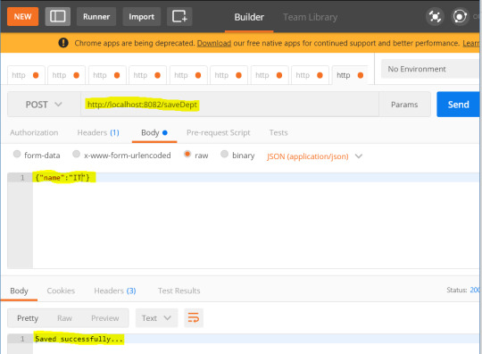
Add students under created department -
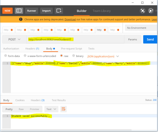
We can check database entries to cross verify -
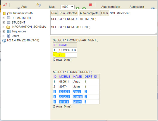
Read the full article
0 notes