#i mean that's more eigenvector than eigenvalue

[abalidoth]

broke: I was sold to One Direction

woke: I was sold one direction

theyre selling WHAT on ebay now

[sunless-not-sinless]

spectral partitioning

i need to do a presentation on spectral partitioning for uni so here we go! an explanation on this graph partitioning algorithm here so i dont forget shit (i will not be looking at random walks)

under the cut theres gonna be maths. a lot of it so if u dont want that then dont look there. and theres no LaTeX or mathjax here so its ugly.

also i assume you know what graphs and eigen-shit are

i will assume our graph is a simple undirected graph.

the core idea of spectral partitioning is minimising the cut size - the sum of weights of the edges between two communities.

so if we have a graph that looks like this

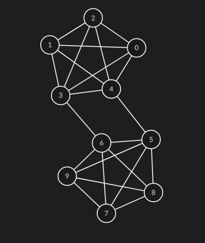
(made on https://csacademy.com/app/graph_editor/)

and we try to cut it into 2 groups, (by inspection) the minimum number of edges we have to cut through is 2, between nodes 3-6 and 4-5. so the minimum cut size is 2. and if we cut through those nodes we get 2 communities.

ill let you convince yourself that minimising the cut will lead to communities that arent very related to each other.

but how do we find this minimum cut? if we try to brute force it then you first separate nodes into one of 2 groups, then sum the weights of edges between nodes in these 2 groups. this is slow - O(2^n) where n is number of nodes in the graph - and it cant be improved (its an np-hard problem).

so instead of optimising that mess we will try to approximate it. sure our approximations might not find the actual minimum cut size but itll be good enough.

now to try to approximate this we need to find a nicer way of writing the cut size of some partition.

let A be the set of nodes in one group of the partition, and Ac its complement (the other group of the partition)

also let A=(w_ij) be a matrix where w_ij is the weight of the edge between nodes i and j (this is called the adjacency matrix, hence the A). and D be the diagonal matrix of "degrees" (actually sum of weights of all adjacent edges, but lets just call it the degree) of nodes.

finally let x be the indicator vector where x_i = 1 if i is in A, else -1. and 1 be the vector of just 1s if i use 1 where you would expect a vector (polymorphism? in my maths? more likely than you think)

and the transpose will be denoted ^T as usual

now to get the cut size, its the sum of edges between A and Ac. so thats ((1+x)/2)^T A ((1-x)/2)

you can probably see the halves are annoying, so lets find 4 * the cut size. so thats (1+x)^T A (1-x)

but this +x -x is a bit weird. it would be better if they were the same sign. so how do we do that?

the sum of weights of edges between the parts of the partition is the same as the all the sum of degrees of nodes minus the sum of weights of nodes within the same group. so we can rewrite this as (1+x)^T D (1+x) - (1+x)^T A (1+x) = (1+x)^T (D-A) (1+x)

now let L = D-A. this is called the laplacian of the graph and it has a few nice properties. first the row/column sums are 0 (you add the "degree" then take away all the weights). second its quadratic form v^T L v = ½ Σ w_ij (v_i - v_j)². importantly this means its positive semi-definite. third its symmetric. importantly this means that it has an orthonormal eigenbasis.[1]

now because its row/column sums are 0 you can write 4 * cut size as (1+x)^T L (1+x) = x^T L x. and so this is what we want to minimise.

now like i said minimising this is np-hard, but we can ignore the fact that x_i = ±1, and instead consider it on all vectors s, then just look at the sign of the entry.

just two issues with this. one: what if theres a 0? well you can lob it in either group of the partition. two: (ks)^T L (ks) = k² x^T L x. so any minimum we find, we can just halve each value of the vector or smth and get a smaller min. for this we can simply consider vectors s.t. ||s||=1.

now we can write s in orthonormal eigenbase to get that s^T L s is a weighted average of the eigenvectors of L. so the minimisation of this is the smallest eigenvalue of L. but because the row/column sums are 0, this eig val is 0 with eig vec being the vector of ones. if you think of this in terms of graphs this makes sense - to minimise the cut you put everything in one bucket and nothing in the other and so theres no edges to cut!

now lets assume a good partition will cut it roughly in half. we can think of this as the number of nodes in one half of the partition. in other words 1^T x ≈ 0. so lets add the constraint that 1^T s = 0.

this means s is orthogonal to 1 - our smallest eigenvector. so in our weighted average, we cannot have any weight for out smallest eigenvalue, and so our second smallest eigenvalue is the smallest and we can approximate the minimum cut size by looking at the signs of the second smallest eigenvector!

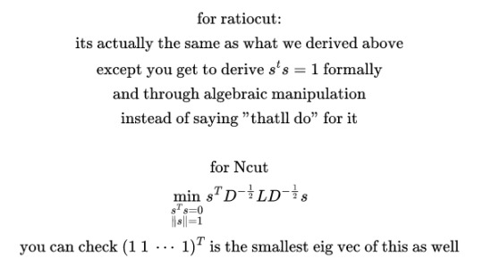
and that is the idea behind spectral partitioning! now you can normalise the cut in some way. e.g.

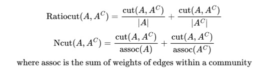
with their associated minimisations being shown below

then you get good algs for separating images into blocks of focus

(sorry for no IDs for these)

and there we go! thats spectral partitioning!

[1] you can use gram schmidt to get an orthogonal basis of an eigen space, so all we need to show is that eig vecs with diff eig vals are orthogonal.

therefore any eig basis of symm (or hermitian) matrix is orthogonal.

the fact that an eigenbase even bloody exists is beyond this tumblr post, but is called the spectral theorem - and is where the name spectral partitioning comes from

[pazodetrasalba]

Iceberg

Dear Caroline:

Long day, today. I've been working with characteristic polynomials, eigenvalues, eigenvectors, adjugate matrices and diagonalizations, so I'll be a bit brief, even though this is a rather complex and controversial topic you we wading in - the stuff that gets easily misread and employed as a weapon against you.

My experience is similar to yours, but the sample is probably biased - most of my male friends and acquaintances are very civilized people with very low inclinations to violence. That does not mean that these situations might not happen in significant numbers, and that some percentage of those fears of male violence might not be unfounded.

Personally, I find it the idea of having sex with a person who is less than fully enthusiastic unerotic and unappealing, but if I would get somewhat upset and disappointed if, after big courtship escalation and all the signals having been clear, I was to be stopped in the tracks. At the very least I would expect some reasonable explanation, and would be tempted to suspect some weird sh*t testing otherwise. I once had a girlfriend who did exactly that, and argued a pretty convincing case for intimacy-avoidance on the premises that 1) she was a very religious and practicing Catholic, and 2) She had had bad experiences in the past. And in the end, the relationship didn't work out and I broke up with her (despite liking her a lot), as I couldn't really trust her argument, or avoid the gnawing thought that if she actually found me more physically attractive, she wouldn't be so remiss about lovemaking.

I am a bit surprised by those thought processes of yours you mention ("well it seems really awkward to say no right now … I mean it’s not like a big deal … I don’t want to make things weird …"), as I really can't imagine myself using them in similar context, so perhaps it's one of those issues of male vs female psychology that we find so difficult to understand at times, as our natural bias is to consider the Other as just like us, but with skirts and slightly modified physical attributes.

Quote:

You never really understand a person until you consider things from his point of view.

Harper Lee

[nostalgebraist]

There is probably no name more liberally and more confusingly used in dynamical systems literature than that of Lyapunov (AKA Liapunov). Singular values / principal axes of strain tensor JJ (objects natural to the theory of deformations) and their longtime limits can indeed be traced back to the thesis of Lyapunov [ 10, 8], and justly deserve sobriquet ’Lyapunov’. Oseledec [8] refers to them as ‘Liapunov characteristic numbers’, and Eckmann and Ruelle [11] as ‘characteristic exponents’. The natural objects in dynamics are the linearized flow Jacobian matrix J t , and its eigenvalues and eigenvectors (stability exponents and covariant vectors). Why should they also be called ’Lyapunov’? The covariant vectors are misnamed in recent papers as ‘covariant Lyapunov vectors’ or ‘Lyapunov vectors’, even though they are not the eigenvectors that correspond to the Lyapunov exponents. That’s just confusing, for no good reason - Lyapunov has nothing to do with linear stability described by the Jacobian matrix J, as far as we understand his paper [10] is about JJ and the associated principal axes. To emphasize the distinction, the Jacobian matrix eigenvectors {e(j) } are in recent literature called ‘covariant’ or ‘covariant Lyapunov vectors’, or ‘stationary Lyapunov basis’ [ 12]. However, Trevisan [7] refers to covariant vectors as ‘Lyapunov vectors’, and Radons [ 13] calls them ‘Lyapunov modes’, motivated by thinking of these eigenvectors as a generalization of ‘normal modes’ of mechanical systems, whereas by ith ‘Lyapunov mode’ Takeuchi and Chat´e [ 14] mean {λj, e(j) }, the set of the ith stability exponent and the associated covariant vector. Kunihiro et al. [15] call the eigenvalues of stability matrix (4.3), evaluated at a given instant in time, the ‘local Lyapunov exponents’, and they refer to the set of stability exponents (4.7) for a finite time Jacobian matrix as the ‘intermediate Lyapunov exponent’, “averaged” over a finite time period. The list goes on: there is ‘Lyapunov equation’ of control theory, which is the linearization of the ‘Lyapunov function’, and the entirely unrelated ‘Lyapunov orbit’ of celestial mechanics.

(Cvitanović et. al., Chaos: Classical and Quantum)

I’ve never gotten far enough into this particular stuff to feel the brunt of this particular terminological clusterfuck, but I felt a stab of painful recognition reading this, because this sort of thing happens all the time

One of the little frustrations of grad school was simultaneously holding in mind (broadly justified) sense that all the profs and paper-authors were far, far smarter than me and the (also justified) sense that they were very sloppy writers and it was my job to clean up their thoughts inside my own head, because they weren’t going to do it for me

[irregularwebcomic]

[Irregular Webcomic! #2011 Rerun](https://ift.tt/36rVt0J)

An Eigen Plot is a story plot that is carefully designed so that every skill of every one of the protagonists, no matter how unlikely or normally useless a skill it is, is needed at some point to overcome an obstacle that would otherwise prevent the heroes from achieving their goal. There are many examples of such plots in fiction. The whole point being, of course, to make sure that each character has something important to do in the story.

The name "Eigen Plot" is taken from a set of concepts in mathematics, namely those of eigenvectors, eigenvalues, and eigenspaces.

Recall from the annotation to strip #1640 that a function is merely a thing that converts one number into another number. But actually, that's not all a function can do. You can extend this definition to say that a function is something which converts any thing into some other thing.

For example, imagine a function that converts a time into a distance. Say I walk at 100 metres per minute. Then in 3 minutes, I can walk 300 metres. To find out how far I can walk in a certain number of minutes, you apply a function that multiplies the number of minutes by 100 and converts the "minutes" to "metres".

That's a pretty simple example, and we could have done pretty much the same thing with a function that simply converts numbers by multiplying them by 100. But let's imagine now that I'm standing in a field with lots of low stone walls running in parallel from east to west. If I walk east or west, I am walking alongside the walls, and never have to climb over them. So I walk at my normal walking speed, and I still walk at 100 metres per minute. But if I walk north or south, then I have to climb over the walls to get anywhere. The result is that I can only walk at 20 metres per minute in a northerly (or southerly) direction.

So, put me in the middle of this field. Now, what function do I need to use to tell me how far I can walk in a given time? You might think that I need two different functions, one multiplying the time by 100, and another multiplying it by 20. But we can combine those into one function by making the function care about the direction of the walking. This is a perfectly good function:

If I am walking east or west, multiply the time by 100 and convert "minutes" to "metres"; if I am walking north or south, multiply the time by 20 and convert "minutes" to "metres"

What happens if I want to walk at an angle, like north-east? If the walls weren't there, I could just walk for a minute to the north-east, and end up 100 metres north-east of where I started. To figure out the equivalent in the walled field, let's break it up into walking east for a bit, and then north for a bit. On the empty field, I would need to walk east 100/sqrt(2) metres (about 71 metres), and then north 100/sqrt(2) metres. In terms of time, the equivalent of walking for 1 minute north-east is walking for 1/sqrt(2) minutes (about 42.4 seconds) east and then 1/sqrt(2) minutes north. It takes me longer (because I'm not walking the shortest distance to my destination), but the end result is the same.

But what happens if I walk for 1/sqrt(2) minutes east and then 1/sqrt(2) minutes north on the field with the walls? I end up 100/sqrt(2) metres east of where I started, but only 20/sqrt(2) metres north of where I started (because the walls slow me down as I walk north). The total distance I've walked is only a little over 72 metres, and my bearing from my starting position, rather than being north-east (or 45° north of east) is only 11.3° north of east. So the function I've described above converts a time of "1 minute north-east" into the distance "72 metres, at a bearing 11.3° north of east". An interesting function!

Here's where we come to the concept of eigenvectors. "Vector" is just a fancy mathematical name for what is essentially an arrow in a particular direction. A vector has both a length and a direction. So a vector of "1 metre north" is different from a vector of "1 metre east". And "1 metre north" is also different from a vector of "1 minute north", by the way. Okay, now we know what a vector is. What's an eigenvector?

Firstly, an eigenvector is a property of a function. Eigenvectors don't exist all by themselves - they only have meaning in the context of a particular function. That's why I went to all the bother of describing a function above. Without a function, there are no eigenvectors. Some functions have eigenvectors, and some functions don't. Okay, ready?

An eigenvector of a function is a vector that does not change direction when you apply the function to it.

An example eigenvector of our function is "1 minute east". The function changes this to "100 metres east". The direction has not changed, therefore "1 minute east" is an eigenvector of our function. Similarly, "1 minute north" is an eigenvector, because the function changes it to "20 metres north". However, "1 minute north-east" gets changed to "72 metres, at a bearing 11.3° north of east" - the direction of this vector is changed, so it is not an eigenvector of our function. In fact, vectors pointing in any direction other than exactly north, south, east, or west are changed in direction by our function, so are not eigenvectors of the function.

But the vector "2 minutes north" gets changed to "40 metres north". So "2 minutes north" is also an eigenvector of the function, just as "1 minute north" is. You've probably realised that any amount of time in the directions north, south, east, and west are also eigenvectors of the function. Our function has an infinite number of different eigenvectors.

Now we're ready to talk about eigenvalues. Again, eigenvalues are properties of a function. They don't exist without a function.

An eigenvalue of a function is the number that an eigenvector is multiplied by in order to produce the size of the vector that results when you apply the function to it.

What are the eigenvalues of our function? Well, if I walk east (or west), we need to multiply the number of minutes by 100 to get the number of metres I walk. This is true no matter how many minutes I walk. So the number 100 is an eigenvalue of the function. And if I walk north (or south), I multiply the number of minutes by 20 to get the number of metres. So the number 20 is an eigenvalue of the function.

These are the only two eigenvalues of the function: 100 and 20. I don't have to worry about vectors in any other directions, because none of those vectors are eigenvectors. And now we come to the idea of eigenspaces. Once more, eigenspaces are properties of functions.

An eigenspace of a function is the collection of eigenvectors of a function that share the same eigenvalue.

In our case, all of the eigenvectors east and west have the eigenvalue 100. So the collection of every possible number of minutes east and west forms one of the eigenspaces of the function. Similarly, all of the eigenvectors north and south share the eigenvalue 20, so make up a second eigenspace of our function. Considering the sets of eigenvectors together, the two eigenspaces of our function are a line running east-west, and a line running north-south, intersecting at my starting position.

[As an aside, let's examine briefly the walking function in a field without walls. In that case, no matter what direction I walk, I walk 100 metres per minute. "1 minute north-east" becomes "100 metres north-east". So every time vector ends up producing a distance vector in the same direction, with the number of metres equal to 100 times the number of minutes. In other words, every time vector, in every direction, is an eigenvector, with an eigenvalue of 100. This function has a lot more eigenvectors that the walled-field function, but only one eigenvalue! Which means there is only one eigenspace, but it isn't just a line in one direction, it's the whole field!]

You'll notice that the two eigenspaces of the walled-field walking function (the north-south line and the east-west line) end up aligned very neatly with the structure of the walls in the field. In general, this is true of many interesting functions in real life applications such as physics, engineering, and so on. In many fields, there are functions that describe various physical properties of things in multiple dimensions.

An example is the stretching of fabric. If you pull a fabric with a certain amount of force, it stretches by a certain amount. The amount it stretches is actually different, depending on what angle you pull at the fabric. (Anyone who does knitting or sewing will know this is the case.) You can describe this with a function that depends on the angle at which you apply the force. Once you have this function (and you could get it, for example, by actually measuring the stretching of a piece of fabric with various different forces and angles), you can calculate the eigenvectors, eigenvalues, and eigenspaces of the function. And it turns out that the eigenvectors, eigenvalues, and eigenspaces of the stretching function will be closely related to actual physical properties of the fabric, such as the directions of the weave.

A very similar case happens in three dimensions with the properties of rocks. By using seismic probing, core sampling, and other techniques, geologists can build up a three-dimensional analogue of a "stretching function" for rocks. And by calculating the eigenvectors of this function, they can figure out the directions of various features within the rocks, such as fault lines. (This is rather simplified, but that's one of the basic principles behind experimental geophysics.)

We have some loose ends to tie up. Where does the name "eigen" come from? This is actually a German word, meaning "own", in the adjectival form. So an eigenvector is an "own-vector" of a function - a vector that belongs to the function. As you can see, this is a very fitting description. The prefix "eigen" has come from this usage into (geeky) English to refer to other characteristic properties of things. One example is eigenfaces, which refers to the characteristic facial feature patterns used in various computerised facial recognition software functions.

Another example is the TV Tropes coinage of the trope Eigen Plot, which began this annotation. This is an abstracted usage, playing off the "characteristic property" implication of the "eigen" prefix. The characters in a story have a certain set of skills, so an eigen-plot is a plot that is characteristic of that set of skills (i.e. one that will exercise all of the skills).

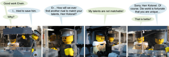
This anotation has no relevance to today's strip, other than that Colonel Haken and Erwin are German, like the word "eigen".

2019-11-03 Rerun commentary: It's interesting that Erwin is driving the truck... but he was just out on the roof fighting with Monty, and is only shown climbing back into the truck here in panel 1. I guess Haken used his hook to steer and just jammed his left foot down on the accelerator while the fight was happening.

[rebrobindoesmath]

How I Attempted to Mathematically Model the Spread of Memes on the Internet, pt 2.

Welcome back! If you’re new to my blog and haven’t read part 1 of this series, you can find it here. 

Now we know enough about Markov chains to start using them to model the spread of memes! This part of the series will primarily involve setting up the model. Here’s a brief outline:

SIR Models

From SIR Model to Meme Model

Woah, Equations!

Coming Up Next

Let’s begin!

SIR Models

In my first post, I stated that my project was originally focused on using Markov chains in disease modeling. My plan was to take SIR Models and adapt them to Markov chains. I ultimately ended up taking this same Markov chain adaptation and using it for my meme model.

I’ll start by discussing SIR Models in general and then we’ll get into Markov chain stuff.

SIR Models are typically used with differential equations to model the spread of infectious diseases. The name comes from the three equations that are used in the model. 

S(t) = S - for susceptible. This function plots the number of individuals that have not become infected with the disease. 

I(t) = I - for infected. This function plots the number of individuals that are currently infected with the disease. 

R(t) = R - for recovered. This function plots the number of individuals that have recovered from having the disease. 

I won’t go into the differential equation version of these, but I definitely encourage you to delve more into them if you’re interested. 

How do these correspond to Markov chain states?

Good question. For my Markov chain adaptation of these equations, my three states come from those three equations. My states are: susceptible ( S ), infected ( I ), and recovered ( R ). 

From SIR Model to Meme Model

What do SIR Models and memes have to do with each other?

Here’s how I connected the two. I’m essentially viewing the spread of a meme over the Internet as if the meme were a disease and the Internet was a population. It’s this connection that drives the rest of this project. We can see that the spread of a meme behaves like the spread of a disease when we look at some graphs. 

First, take a gander at this typical SIR Model graph, paying special attention to I(t). I(t) is the equation that models the population that is infected, which is what we’re really concerned with. 

This I(t) has a strong sharp peak at first and then decreases. This is typical with what we expect with diseases: we have the initial “outbreak” corresponding to the sharp peak, and then as the population begins to recover, I(t) decreases. 

Compare the shape of this I(t) to the shape of the Google Trends graph for the search term “dat boi”. Let’s quickly note that Google Trends plots the popularity of the search term and not the meme, but I think it’s safe to assume that the popularity of the search term is directly related to the popularity of the meme itself. 

Well, hey, they look pretty similar! This is nice because it means we can attempt to use our Markov chain adaptation of SIR Models to try and model this behavior! 

Before we go more in depth, let’s talk about what the states of my Markov chain are in context with memes. 

Susceptible - an individual is in this state if they have not seen the meme in question. 

Infected - the individual is in this state if they have seen the meme and are actively sharing it among peers. 

Recovered - an individual is in this state if they are no longer interested in the meme and are no longer sharing it. 

What does the Markov chain look like?

Here’s a visual for my Markov chain for the SIR Models.

This requires a bit of explaining. S, I, and R are the susceptible, infected, and recovered states respectively. The arrows indicate moving from one state to the next, and the probabilities of moving are written next to the arrows. 

For example, an individual moves from the susceptible state to the infected state with a probability $\alpha$. If an individual does not move to the infected state, they stay at the susceptible state with a probability $1-\alpha$. Let’s define our probabilities really quick:

$\alpha$ - the probability of moving from susceptible to infected.

$\beta$ - the probability of moving from infected to recovered.

$\gamma$ - the probability of moving from recovered to infected. 

Using what we learned in the last post, we come up with the following transition matrix, $M$:

A couple quick notes:

Our columns are organized S, I, R from left-to-right. Our rows are similarly organized from top-to-bottom.  

Each $M_{i,j}$ is the probability of going from state $j$ to state $i$. 

Now that we have our transition matrix, we can do ~really cool things~ with it. 

Woah, Equations!

What are these “really cool things”?

The transition matrix itself doesn’t tell me a whole lot of information unless I know what my probabilities are. Because we’re looking at this in general, our specific probabilities are unknown. However, not all hope is lost because I can do some cool tricks that will tell me more. 

Recall that if I want to find the probability of being in state $i$ after starting in state $j$ after n time steps, I just find $M_{i,j}^n$. 

So how can we find $M^n$ without knowing the probabilities? 

Here’s the trick: we diagonalize $M$. That is, I want to find matrices $P$ and $D$ such that $M = PDP^{-1}$. Then when I raise both sides to the nth power, the right side will cancel out so that I’m left with $M^n = PD^nP^{-1}$. $P$ is the matrix of our eigenvectors and $D$ is the diagonal matrix of our eigenvalues. We obtain:

Because $D$ is diagonal, it makes the matrix multiplication a bajillion times simpler. Raising $D$ to the nth power just raises each individual entry in the diagonal to the nth power. 

The entries of $M^n$ that I’m concerned with are the entries in the first column. These are the probabilities of being in each state after starting from the susceptible state. So, I’m only going to perform the matrix multiplication enough to get the first column of $M^n$ (but you’re more than welcome to perform the whole thing if you’d like). 

Additionally, I want to think of these entries as continuous functions (instead of with discrete time steps). This is an extension of the model and will allow me to me to do more ~cool things~. Therefore, I will use the continuous variable t instead of the discrete variable n. 

You can check for yourself, but by multiplying these matrices out, we obtain the following functions (these are the first column entries of $M^n$):

where S(t) is the probability of being in the susceptible state at time t, and the same for I(t) and R(t) for the infected and recovered states respectively. 

If you’re interested, here is a link to a graph on Desmos with sliders for $\alpha$ ( a ), $\beta$ ( b ), and $\gamma$ ( c ) you can play with. 

Now that we have these equations, we can attempt to model the spread of a meme! However, for the sake of length, we’ll save this for next time.

Coming Up Next

Next, we’ll talk a little bit more about these equations, specifically I(t). Additionally, we’ll take data from Google Trends and attempt to find the $\alpha$, $\beta$, and $\gamma$ that will best fit our I(t) equation to the data. We’ll also try to see if there is any way we can predict what $\alpha$, $\beta$ and $\gamma$ could be from an initial set of data points. Stay tuned!

Thanks for reading!

As always, if there are any questions/comments/concerns, feel free to send an ask. 

Hope all is well!

Update: Here is Part 3 (The Final Chapter) of this series. 

Where I Got My Pictures From

SIR Model Graph

Google Trends (which is actually super fun to just play around with)

[gtzfinance]

Hermitian Matrices and the Fallacy of Simpler Solutions

Author:

Thomas Becker

Prerequisites:

The first part of this post is a general interest musing with no prerequisites. The second part is mathematical and assumes the mathematical maturity of a technical person as well as a working knowledge of linear algebra. This post is not related to finance.

Summary:

This blog post argues that the urge to simplify and streamline other people's computer code or mathematical work is almost always misguided. However, we claim that hunting for the simplest proofs of established mathematical results has some value. We show a simple proof of the spectral theorem for hermitian matrices as an example.

The Fallacy of Simpler Solutions

I am a mathematician and a software engineer. Therefore, I tend to have the bad habits of both groups. In particular, like many software engineers, I have been known to point my finger at other people's working code and proclaim that I could simplify it, making it more elegant, efficient, readable, and maintainable. Similarly, looking at other mathematician's papers or textbooks sometimes makes me want to declare that I could do the same thing in a way that's shorter, simpler, more readable, easier to understand, and so on, you get the picture.

As I've grown wiser and more mature over the years, I have installed a little voice in my head that comes on every time that I feel the urge to level this kind of criticism at someone. The voice reminds me of the FSS, the Fallacy of Simpler Solutions:

1. Embellishing something when someone else has done the heavy lifting is easy. In fact, if my criticism has any virtue at all, the person who did the original work would probably see the same thing if they went back to it now. But they don't, because they're off doing more original work while I'm nitpicking on other people's achievements. So first off, no reason to be all condescending and sanctimonious.

2. The existing solution that I'm looking at works. Mine is an idea that popped into my head just now. By the time it's all written down or implemented, it may not be so simple anymore. In fact, it may not even work at all. [1]

3. A solution that I come up with will almost necessarily seem simpler and more elegant to me, because it's mine and corresponds naturally to my way of thinking. Other people may not see it that way. What I have may be just an alternate solution, not a simpler one.

4. Even assuming that my solution is simpler, more elegant, more efficient, and all that, is it really worth making a big deal of it, and, in the case of a computer program, to actually modify the code? It almost never is. [2] Putting everybody through that painful process of finding and fixing all the little mistakes and bugs all over again? For what? What's the gain? In the vast majority of cases, the only gain is that my pompous ego can feel better about itself. Great.

5. Don't fix it if it ain't broke.

So, long story short, I try not to waste any precious time going around telling other people that I could have done their work better, if only I had done it at all. There is only one way to put my insights, if any, to good use, and that's by applying them in my own original work. Now there's a real value-add. And besides, what's a better way of bringing my insight to other people's attention: demonstrating its value by applying it myself, or nitpicking on their achievements?

However, it just recently occurred to me that in the case of mathematical proofs, hunting for simpler proofs of established results can make sense and lead to valuable insight, if one understands what one is doing. The following discussion of simplifying mathematical proofs uses the the spectral theorems for operators on finite-dimensional vector spaces (i.e., diagonalization of matrices) as its main example. I will therefore have to assume that you already know pretty much everything about linear algebra up to and including eigenvectors, eigenvalues and spectral theorems.

Simplifying Proofs by Discarding Generality

Suppose you're looking up the proof of the spectral theorem for hermitian matrices in a linear algebra textbook. What should you find? The book will of course have a proof of the spectral theorem for normal matrices. It wouldn't be a good textbook if it didn't. But once you have a proof of the spectral theorem for normal matrices, the spectral theorem for hermitian matrices is an easy corollary because a hermitian matrix is clearly normal. All you have to do is add an almost trivial remark regarding the eigenvalues of a hermitian matrix being real.

So now your proof of the spectral theorem for hermitian matrices consists of a proof of the spectral theorem for normal matrices plus some trivial remarks. That's not the simplest possible proof. If you shoot for hermitian matrices directly, disregarding the more general case of normal matrices, you can get a simpler proof, as will be demonstrated below. But you certainly wouldn't criticize the textbook author for not presenting that proof. Why would she? It would be a waste of time, and it would make the textbook look messy. Still, there is value in looking at the simpler proof: it gives you an intuition for how much deeper the spectral theorem for normal matrices is than the one for hermitian matrices. Not everybody may be interested in developing that intuition, but it's additional insight nonetheless. And if nothing else, it makes for great recreational mathematics. If I were to go back to teaching or textbook authorship, which is not likely to happen, I would try to stuff the exercise sections with such simpler proofs of more specialized results. [3]

Simplifying Proofs by Discarding Constructivity

The proofs of the spectral theorems in linear algebra textbooks are typically centered around the determinant and the characteristic polynomial of a matrix, and the Cayley-Hamilton Theorem. It is possible to prove the spectral theorems without the use of all that, resulting in dramatically simpler proofs. This will be demonstrated below for the special case of hermitian matrices. So does that mean that pretty much every linear algebra textbook ever written is full of unnecessarily complicated proofs? Of course not. The simpler proofs, like the one presented below, prove the existence of a unitarily equivalent diagonal matrix. But linear algebra, perhaps more so than any other branch of mathematics, is not just about the existence of things. It is a tool for applied physicists and engineers who need to calculate stuff like equivalent diagonal matrices and solutions to linear equations. The characteristic polynomial, and thus, by implication, the Caley-Hamilton Theorem, are indispensible tools in these efficient calculations. Therefore, presenting the spectral theorems without bringing in the characteristic polynomial would be kind of missing the point. Nonetheless, I believe that looking at the simpler proof still has value: it gives you an intuition for how much deeper the problem of (efficient) computation is, as opposed to just proving existence. [4] And again, it makes for some fun recreational mathematics.

In the case of the spectral theorems for linear operators on finite-dimensional vector spaces, the simpler proofs are still constructive, meaning they still provide a method of calculating the diagonalizations (modulo the problem of calculating zeroes of polynomials, of course). They just completely disregard the efficiency of the calculation. There are other examples of simplified proofs where the original proof is constructive, while the simpler one is no longer constructive at all. [5]

Diagonalization of Hermitian Matrices

During one of my recent peregrinations in the American Desert Southwest, my mind, trying to distract itself from the pain caused by my body carrying a multi-day pack with three gallons of water added, started wondering if it could prove the spectral theorem for Hermitian operators on finite-dimensional vector spaces (diagonalization of Hermitian matrices) without looking anything up.

When it was done I was convinced that I must have made a mistake, it was so simple. Of course calling a proof simple makes sense only if you specify what exactly you assume to already be known. For example, the spectral theorem for Hermitian operators would be trivial if you were to assume the spectral theorem for normal operators to be already known. As you will see in a moment, the simple proof that I'm talking about assumes only the most elementary results on basis and dimension, linear maps and matrices, orthogonality, stuff like that, things that you learn in a first undergraduate course on linear algebra. And, perhaps somewhat importantly, you can even subtract everything regarding the determinant from that.

There is, of course, the small matter of the Fundamental Theorem of Algebra, i.e., the fact that every non-constant polynomial over the complex numbers has a zero. That cannot be simplified away from the spectral theorems. In fact, in view of the proof below, one is tempted to say that diagonalization of Hermitian matrices is no more than a corollary to the Fundamental Theorem of Algebra.

Before we go, allow me to emphasize again that if you're teaching a course or writing a textbook on linear algebra, this is most definitely not the kind of proof you want to present, for two reasons:

1. This proof lacks generality. You want to obtain the spectral theorem for Hermitian operators as a special case of the spectral theorem for normal operators.

2. This proof under-emphasizes efficiency of computation. Diagonalization of matrices is a very practical matter, and therefore should be taught with an eye on real-world calculations. This means you must bring in the determinant, the characteristic polynomial, and the Cayley-Hamilton Theorem.

However, this proof could make for a nice sequence of exercises or homework assignments, and for me, it's fun recreational mathematics.

One last thing before we delve into the math. To preempt any misunderstandings, let me stress that there is nothing even remotely original about the proof that you'll see below. I just think it's fun to arrange things so that you see clearly what specific arguments are needed above and beyond elementary linear algebra.

In this section, \(V\) shall be a finite-dimensional vector space over \(\mathbb{C}\), and the term operator, or complex operator for clarity, shall mean an endomorphism on \(V\). Complex operators thus correspond to complex square matrices. I will assume that you know what it means for a complex operator or square matrix to be hermitian. We want to prove the following theorem:

Theorem 1: If \(A\) is a hermitian operator, then \(V\) has an orthonormal basis of eigenvectors of \(A\), and all eigenvalues of \(A\) are real.

In terms of matrices, the theorem states that a hermitian matrix is unitarily equivalent to a real diagonal matrix.

The proof of the theorem hinges on the following two propositions:

Proposition 1: Let \(A\) be a hermitian operator and \(U\) a subspace of \(V\). If \(U\) is invariant under \(A\), the so is its orthogonal complement \(U^{\perp}\).

Proposition 2: Every complex operator has an eigenvector.

Here's how Theorem 1 follows from the two propositions:

Proof of Theorem 1: Let \(A\) be a hermitian operator. It is easy to see that any eigenvalue of \(A\) must be real: if \(e\) is an eigenvector with eigenvalue \(\lambda\), then $$ \lambda (e \cdot e) = \lambda e \cdot e = A e \cdot e = e \cdot A e = e \cdot \lambda e = \bar{\lambda} (e\cdot e) $$ and therefore, \(\lambda = \bar{\lambda} \). The proof that \(V\) has an orthonormal basis of eigenvectors of \(A\) is by induction on \(\dim(V)\). The case \(\dim(V) = 1\) is trivial. Let \(\dim(V) > 1\), and let \(e\) be an eigenvector of \(A\). We may assume that \(\| e \| = 1 \). Since the generated subspace \(\langle e \rangle\) of \(V\) is invariant under \(A\), so is its orthogonal complement \(\langle e \rangle^\perp\). Trivially, the restriction of \(A\) to \(\langle e \rangle^\perp\) is again hermitian, and therefore, by induction hypothesis, \(\langle e \rangle^\perp\) has an orthonormal basis of eigenvectors of that restriction. Trivially, these eigenvectors are also eigenvectors of \(A\), and each of them is orthogonal to \(e\). Therefore, together with \(e\), they form an orthonormal basis of \(V\) consisting of eigenvectors of \(A\). q.e.d.

It remains to prove the two propositions. The first one is near trivial:

Proof of Proposition 1: Let \(A\) be a hermitian operator, and let \(U\) be an \(A\)-invariant subspace of \(V\). If \(v\in U^\perp\), then, for all \(w\in U\), $$Av \cdot w = v \cdot Aw = 0,$$ and thus \(Av\in U^\perp \). q.e.d.

Proof of Proposition 2: The set of operators on \(V\) forms a vector space with the natural operations of adding operators and multiplying them by complex numbers. This vector space has dimension \(n^2\) where \(n\) is the dimension of \(V\). This is most easily seen by using the one-to-one correspondence to \(n\times n\) matrices: any \(n\times n\) matrix is a sum of multiples of matrices that have one entry 1 and all other entries 0. It follows that the operators \(A^0, A^1, A^2,\ldots , A^{n^2}\) are linearly dependent. This means that there is a polynomial \(p\in \mathbb{C}[X]\) such that \(p(A)\) is the null operator. [6] We may assume that \(p\) is a polynomial of minimal degree with that property. Let \(\lambda\) be a complex zero of \(p\), and let \(q\in \mathbb{C}[X]\) such that \(p = (X - \lambda) q\). By the minimality of the degree of \(p\), \(q(A)\) is not the null operator, and thus there exists \(v\in V\) with \(q(A) v \neq 0\). It follows that \(q(A) v\) is an eigenvector of \(A\) with eigenvalue \(\lambda\): $$ (A - \lambda)((q(A) v) = ((A - \lambda)(q(A)) v = p(A)v = 0. $$ q.e.d.

For completeness' sake, I should mention that the converse of Theorem 1 is true too: you can easily convince yourself that a complex matrix that is unitarily equivalent to a real diagonal matrix is hermitian.

Diagonalization of Symmetric Matrices

We can't very well leave the topic of hermitian matrices without mentioning real symmetric operators and matrices. So let us change the setup of the previous section by replacing \(\mathbb{C}\) with \(\mathbb{R}\), which means that we're now looking at real symmetric operators and matrices instead of complex hermitian ones. It turns out that the perfect analogue to Theorem 1 is true:

Theorem 2: If \(A\) is a symmetric operator, then \(V\) has an orthonormal basis of eigenvectors of \(A\).

In terms of matrices, the theorem states that a real symmetric matrix is unitarily equivalent to a real diagonal matrix, with the transformation matrix being real as well.

Notice that Theorem 2 is not a plain special case of Theorem 1. You may view a real symmetric matrix as a complex hermitian matrix and apply Theorem 1. But it is not obvious that the transforming matrix can be chosen to be real as well. So what's the simplest and/or most enlightening proof of Theorem 2? One thing you can do is repeat the proof of Theorem 1. The only difference happens when it comes to Proposition 2, the existence of an eigenvector. You can refine the proof of Proposition 2 to show that there actually exists a real eigenvector. That's all you need. That way, the proof of Theorem 2 is a slightly longer and more complicated version of the proof of Theorem 1.

But that's not the whole story. Suppose that we had taken the classic constructive, calculation-oriented approach to Theorem 1. Then we would have obtained that orthonormal basis of eigenvectors not by some rather abstract proof by induction, but as the union of bases of the different eigenspaces. And the basis of an eigenspace, in turn, is obtained by solving a system of linear equations, namely, \((A - \lambda)x = 0\), where \(\lambda\) is the eigenvalue. We already know that eigenvalues of hermitian matrices are real. So if \(A\) happens to be real as well, then the system of linear equations \((A - \lambda)x = 0\) is all real, and solving it won't take us outside of the real numbers. And voilà, Theorem 2 just happened, by inspecting the proof of Theorem 1. [7] Perhaps the constructive approach is not so uncool after all.

Notes

[1]

This is somewhat reminiscent of Joel Spolsky's famous blog post in which he argues that simplicity and elegance of code tend to not survive contact with users.

[2]

And again, I have to hand it to Joel Spolsky's for having argued this point already, and better at that.

[3]

Perhaps my favorite of those simplified-by-discarding-generality proofs is the direct proof of the formula for the sum of the infinite geometric series. Of course we all want to know what the sum of the finite geometric series is. So we do that first, and once we know what it is, namely, \((1-r^n)/(1-r)\), it follows immediately that the sum of the infinite geometric series is \(1/(1-r)\). Few people (the author of "The Revenant" apparently being one of them) seem to know that there's a beautifully simple and intuitive direct proof of the formula for the infinite geometric series. This blog post has more about that.

[4]

There is actually a linear algebra textbook that prides itself in banning the concept of the determinant to the end of the book (Linear Algebra Done Right, by Sheldon Axler). I enjoyed perusing the book; its agenda of simplifying the proofs of results such as the spectral theorems is carried out brilliantly. I do take issue with the title, though. It is hard for me to imagine a group of students that is served well by teaching them linear algebra without emphasis on the tools needed for efficient calculations.

[5]

In a 1989 article in the Notices of the American Mathematical Society, George Boolos presented a proof of Goedel's First Incompleteness Theorem based on the Berry Paradox that is much simpler than Goedel's original proof (Notices Amer. Math. Soc. 36, 1989, 388–390). The article spawned passionate discussions, carried out in letters to the editor as well as in math departments all over the world. (Social media wasn't a thing back then.) It took quite a while until a consensus emerged that Boolos' proof is simpler because it is non-constructive, i.e., it proves the existence of a statement that is neither provable nor disprovable without providing a way to construct such a sentence. Nonetheless, Boolos' proof is widely considered a valid original contribution, because it sharpens our understanding of the depth and ramifications of Goedel's results.

[6]

This is where the computational inefficiency of this proof's approach really jumps out at you: you'd be a fool to compute an annihilating polynomial in this manner. You'd use the characteristic polynomial of course. But in terms of simplicity of proof, you lost bigtime, because you just bought yourself the Cayley-Hamilton theorem.

[7]

Essentially the same argument is used in abstract algebra to prove that if \(K\subset L\) are fields and \(p,q\in K[X]\) are such that \(q∣p\) in \(L[X]\), then \(q∣p\) in \(K[x]\).

[mathematicianadda]

The Big Lock-Down Math-Off, Match 12

Welcome to the 12th match in this year’s Big Math-Off. Take a look at the two interesting bits of maths below, and vote for your favourite.

You can still submit pitches, and anyone can enter: instructions are in the announcement post.

Here are today’s two pitches.

Matthew Scroggs – Interesting Tautologies

Matthew Scroggs is one of the editors of Chalkdust, a magazine for the mathematically curious, and blogs at mscroggs.co.uk. He tweets at @mscroggs.

A few years ago, I made @mathslogicbot, a Twitter bot that tweets logical tautologies.

The statements that @mathslogicbot tweets are made up of variables (a to z) that can be either true or false, and the logical symbols $\lnot$ (not) $\land$ (and), $\lor$ (or), $\rightarrow$ (implies), and $\leftrightarrow$ (if and only if), as well as brackets. A tautology is a statement that is always true, whatever values are assigned to the variables involved.

To get an idea of how to interpret @mathslogicbot’s statements, let’s have a look at a few tautologies:

$( a \rightarrow a )$. This says “$a$ implies $a$”, or in other words “if $a$ is true, then $a$ is true”. Hopefully everyone agrees that this is an always-true statement.

$( a \lor \lnot a )$. This says “$a$ or not $a$”: either $a$ is true, or $a$ is not true.

$(a\leftrightarrow a)$. This says “$a$ if and only if $a$”.

$\lnot ( a \land \lnot a )$. This says “not ($a$ and not $a$)”: $a$ and not $a$ cannot both be true.

$( \lnot a \lor \lnot \lnot a )$. I’ll leave you to think about what this one means.

(Of course, not all statements are tautologies. The statement $(b\land a)$, for example, is not a tautology as is can be true or false depending on the values of $a$ and $b$.)

While looking through @mathslogicbot’s tweets, I noticed that a few of them are interesting, but most are downright rubbish. This got me thinking: could I get rid of the bad tautologies like these, and make a list of just the “interesting” tautologies. To do this, we first need to think of different ways tautologies can be bad.

Looking at tautologies the @mathslogicbot has tweeted, I decided to exclude:

tautologies like \((a\rightarrow\lnot\lnot\lnot\lnot a)\) that contain more than one \(\lnot\) in a row.

tautologies like \(((a\lor\lnot a)\lor b)\) that contain a shorter tautology. Instead, tautologies like \((\text{True}\lor b)\) should be considered.

tautologies like \(((a\land\lnot a)\rightarrow b)\) that contain a shorter contradiction (the opposite of a tautology). Instead, tautologies like \((\text{False}\rightarrow b)\) should be considered.

tautologies like \((\text{True}\lor\lnot\text{True})\) or \(((b\land a)\lor\lnot(b\land a)\) that are another tautology (in this case \((a\lor\lnot a)\)) with a variable replaced with something else.

tautologies containing substatements like \((a\land a)\), \((a\lor a)\) or \((\text{True}\land a)\) that are equivalent to just writing \(a\).

tautologies that contain a \(\rightarrow\) that could be replaced with a \(\leftrightarrow\), because it’s more interesting if the implication goes both ways.

tautologies containing substatements like \((\lnot a\lor\lnot b)\) or \((\lnot a\land\lnot b)\) that could be replaced with similar terms (in these cases \((a\land b)\) and \((a\lor b)\) respectively) without the \(\lnot\)s.

tautologies that are repeats of each other with the order changed. For example, only one of \((a\lor\lnot a)\) and \((\lnot a\lor a)\) should be included.

After removing tautologies like these, some of my favourite tautologies are:

\(( \text{False} \rightarrow a )\)

\(( a \rightarrow ( b \rightarrow a ) )\)

\(( ( \lnot a \rightarrow a ) \leftrightarrow a )\)

\(( ( ( a \leftrightarrow b ) \land a ) \rightarrow b )\)

\(( ( ( a \rightarrow b ) \leftrightarrow a ) \rightarrow a )\)

\(( ( a \lor b ) \lor ( a \leftrightarrow b ) )\)

\(( \lnot ( ( a \land b ) \leftrightarrow a ) \rightarrow a )\)

\(( ( \lnot a \rightarrow b ) \leftrightarrow ( \lnot b \rightarrow a ) )\)

You can find a list of the first 500 “interesting” tautologies here. Let me know on Twitter which is your favourite. Or let me know which ones you think are rubbish, and we can further refine the list…

Colin Beveridge – Binet’s formula and Haskell

Colin blogs at flyingcoloursmaths.co.uk and tweets at @icecolbeveridge.

As ordained by Stigler’s law (which is attributed to Merton), Binet’s formula was known at least a century before Binet wrote about it

Binet’s formula is a lovely way to generate the \( n \)th Fibonacci number, \( F_n \). If \( \phi = \frac{1}{2}\left(\sqrt{5} + 1\right)\), then

\( F_n = \frac{ \phi^n – (-\phi)^{-n} }{\sqrt{5}}\)

Where does it come from?

Which, of course, I’ll leave as an exercise

It’s not hard to prove this by induction, but that feels like a bit of a cheat: it doesn’t explain why Binet’s formula works.

Personally, I like to prove it as follows.

Suppose \( F_{n-1} \) and \( F_{n} \) are consecutive Fibonacci numbers for some integer \( n \).

Then, if I want to end up with \( F_{n} \) and \( F_{n+1} \), I can use a matrix: \( \begin{pmatrix} F_{n} \\ F_{n+1} \end{pmatrix}= \begin{pmatrix} 0 & 1 \\ 1 & 1 \end{pmatrix} \begin{pmatrix} F_{n-1} \\ F_{n} \end{pmatrix} \)

That’s true for any \( n \), and (given that \( F_0 = 0 \) and \( F_1 = 1 \)), I can write: \( \begin{pmatrix} F_{n} \\ F_{n+1} \end{pmatrix}= \begin{pmatrix} 0 & 1 \\ 1 & 1 \end{pmatrix}^n \begin{pmatrix} 0 \\ 1 \end{pmatrix} \)

I only realised fairly recently what was going on when you diagonalise a matrix as \( \mathbf{PDP}^{-1} \). If you apply this to one of the eigenvectors, \( \mathbf{P}^{-1} \) maps it to one of the axes; \( \mathbf{D} \) stretches it by the appropriate eigenvalue; \(\mathbf{P} \) maps it back parallel to the original eigenvector – so applying the diagonalisation to the eigenvector does exactly the same as applying the matrix to it. This is true for the other eigenvector(s), too; and because of all the linear goodness buried in linear algebra, the diagonalisation maps any linear combination of the eigenvectors – which, as long as your matrix has enough eigenvectors, means any vector – the same way as the original matrix does. If you don’t have enough eigenvectors, please consult a linear algebra professional immediately.

I smell an eigensystem – if I diagonalise the matrix, I can use that as a shortcut to unlimited power, bwahaha! (What’s that? Just unlimited powers of the matrix. Fine.) I’ll skip the tedious and arduous calculation required to diagonalise it, and note that: \( \begin{pmatrix} 0 & 1 \\ 1 & 1 \end{pmatrix}^n = \frac{1}{\sqrt{5}} \begin{pmatrix} -\phi & \frac{1}{\phi} \\ 1 & 1 \end{pmatrix} \begin{pmatrix} -\frac{1}{\phi} & 0 \\ 0 & \phi \end{pmatrix}^n \begin{pmatrix} -1 & \frac{1}{\phi} \\ 1 & {\phi} \end{pmatrix} \)

This simplifies (after a bit of work) to: \(\begin{pmatrix} 0 & 1 \\ 1 & 1 \end{pmatrix}^n =\frac{1}{\sqrt{5}} \begin{pmatrix} \phi^{-(n-1)} + \phi^{n-1} & -(-\phi)^{-n} + \phi^n \\ \phi^{-n} + \phi^n & -(-\phi)^{-(n+1)} + \phi^{n+1} \end{pmatrix} \)

And

\(\begin{pmatrix} F_{n} \\ F_{n+1} \end{pmatrix} = \begin{pmatrix} 0 & 1 \\ 1 & 1 \end{pmatrix}^n \begin{pmatrix} 0 \\ 1 \end{pmatrix}= \frac{1}{\sqrt{5}} \begin{pmatrix} \phi^n – (-\phi)^{-n} \\ \phi^{n+1} – (-\phi)^{-(n+1)} \end{pmatrix} \)

… which gives us Binet’s formula \( \blacksquare \)

A brief aside

In fact, it’s very close to \( F_n \), but that’s not the interesting thing here.

A thing that makes me go oo: the numerator of Binet’s formula gives integer multiples of \( \sqrt{5} \), and because \( 0 < \phi^{-1} < 1 \), the value of \( \phi^{-n} \) gets small as \( n \) gets large. As a result, \( \frac{\phi^n}{\sqrt{5}} \) is very close to an integer for even moderately large values of \( n \).

Calculating in \( \mathbb{Q}\left(\sqrt{5}\right) \)

Which I was – the code is interesting, but not Math-Off-interesting

If you were, for example, trying to implement this in Haskell you might consider working in the field \( \mathbb{Q}\left(\sqrt{5}\right) \). You might, having considered that, run away screaming from the frightening notation – but \( \mathbb{Q}\left(\sqrt{5}\right) \) is less distressing than it looks: it’s just algebraic numbers of the form \( a + b \sqrt{5} \), where \( a \) and \( b \) are rational numbers – and addition, subtraction, multiplication and division (by anything that isn’t zero) are all defined as you would expect. You might like to verify that all of these operations leave you with another element of the field.

Another example of a field extension that works a similar way: the complex numbers can be thought of as \( \mathbb{R}(i) \) – numbers of the form \( a + bi \) where \(a \) and \(b \) are real.

In particular, \( \phi\) is an element of this field, with \( a = b = \frac{1}{2} \). Also,\( -\phi^{-1} \) is an element of the field, with \( a = \frac{1}{2} \) and \( b = – \frac{1}{2} \).

A little bit of messing with the binomial theorem tells you that calculating \( \phi^n – \left(-\phi^{-n}\right) \) leaves an element of \( \mathbb{Q}(\sqrt{5}) \) that’s purely a multiple of \( \sqrt{5} \) (it’s of the form \( a + b \sqrt{5} \), but with \( a = 0 )\) – so Binet’s formula gives us something that’s definitely rational.

Suppose, for example, we work out \( \phi^{10} \) and get \( \frac{123}{2} + \frac{55}{2}\sqrt{5} \). (It doesn’t take much more work to figure out that \( (-\phi)^{-10} = \frac{123}{2} – \frac{55}{2}\sqrt{5} \) so that Binet gives 55 as the tenth Fibonacci number.)

The oo! thing for me, though, is the other number. 123 is the tenth Lucas number – which are formed the same way as Fibonacci numbers, but with \( L_0 = 2 \) and \( L_1 = 1 \). It’s not necessarily a surprise that the Lucas and Fibonacci sequences are linked like this, but it does strike me as neat.

Links

Binet’s formula

Lucas numbers

Blazing fast Fibonacci Numbers

So, which bit of maths made you say “Aha!” the loudest? Vote:

Note: There is a poll embedded within this post, please visit the site to participate in this post's poll.

The poll closes at 9am BST on Tuesday the 5th, when the next match starts.

If you’ve been inspired to share your own bit of maths, look at the announcement post for how to send it in. The Big Lockdown Math-Off will keep running until we run out of pitches or we’re allowed outside again, whichever comes first.

from The Aperiodical https://ift.tt/35ogjy0 from Blogger https://ift.tt/3dgUymB

[kanjasaha]

Preparing for a Data Science/Machine Learning Bootcamp

If you are reading this article, there is a good chance you are considering taking a Machine Learning(ML) or Data Science(DS) program soon and do not know where to start. Though it has a steep learning curve, I would highly recommend and encourage you to take this step. Machine Learning is fascinating and offers tremendous predictive power. If ML researcher continue with the innovations that are happening today, ML is going to be an integral part of every business domain in the near future.

Many a time, I hear, "Where do I begin?". Watching videos or reading articles is not enough to acquire hands-on experience and people become quickly overwhelmed with many mathematical/statistical concepts and python libraries. When I started my first Machine Learning program, I was in the same boat. I used to Google for every unknown term and add "for dummies" at the end :-). Over time, I realized that my learning process would have been significantly smoother had I spent 2 to 3 months on the prerequisites (7 to 10 hours a week) for these boot camps. My goal in this post is to share my experience and the resources I have consulted to complete these programs.

One question you may have is whether you will be ready to work in the ML domain after program completion. In my opinion, it depends on the number of years of experience that you have. If you are in school, just graduated or have a couple of years of experience, you will likely find an internship or entry-level position in the ML domain. For others with more experience, the best approach will be to implement the projects from your boot camp at your current workplace on your own and then take on new projects in a couple of years. I also highly recommend participating in Kaggle competitions and related discussions. It goes without saying that one needs to stay updated with recent advancements in ML, as the area is continuously evolving. For example, automated feature engineering is growing traction and will significantly simplify a Data Scientist's work in this area.

This list of boot camp prerequisite resources is thorough and hence, long :-). My intention is NOT to overwhelm or discourage you but to prepare you for an ML boot camp. You may already be familiar with some of the areas and can skip those sections. On the other hand, if you are in high school, I would recommend completing high school algebra and calculus before moving forward with these resources.

As you may already know, Machine Learning (or Data Science) is a multidisciplinary study. The study involves an introductory college-level understanding of Statistics, Calculus, Linear Algebra, Object-Oriented Programming(OOP) basics, SQL and Python, and viable domain knowledge. Domain knowledge comes with working in a specific industry and can be improved consciously over time. For the rest, here are the books and online resources I have found useful along with the estimated time it took me to cover each of these areas.

Before I begin with the list, a single piece of advice that most find useful for these boot camps is avoid going down the rabbit hole. First, learn how without fully knowing why. This may be counter-intuitive but it will help you learn all the bits and pieces that work together in Machine Learning. Try to stay within the estimated hours(maybe 25% more) I have suggested. Once you have a good handle on the how, you will be in a better position to deep five into each of the areas that make ML possible.

Machine Learning:

Machine Learning Basics - Principles of Data Science: Sinan Ozdemir does a great job of introducing us to the world of machine learning. It is easy to understand without prior programming or mathematical knowledge. (Estimated time: 5 hours)

Applications of Machine Learning - A-Z by Udemy: This course cost less than $20 and gives an overview of what business problems/challenges are solved with machine learning and how. This keeps you excited and motivated if and when you are wondering why on earth you are suddenly learning second-order partial derivatives or eigenvalues and eigenvectors. Just watching the videos and reading through the solutions will suffice at this point. Your priority code and domain familiarity. (Estimated time: 2-3 hours/week until completion. If you do not understand fully, that is ok at this time).

Reference Book - ORielly: Read this book after you are comfortable with Python and other ML concepts that are mentioned here but not necessary to start a program.

SQL:

SQL Basics - HackerRank: You will not need to write SQL as most ML programs provide you with CSV files to work with. However, knowing SQL will help you to get up to speed with pandas, Python's data manipulation library. Not to mention it is a necessary skill for Data Scientists. HackerRank expects some basic understanding of joins, aggregation function etc. If you are just starting out with SQL, my previous posts on databases may help before you start with HackerRank. (Estimated time: Couple of hours/week until you are comfortable with advanced analytic queries. SQL is very simple, all you need is practice!)

OOP:

OOP Basics - OOP in Python : Though OOP is widespread in machine learning engineering and data engineering domain, Data Scientists need not have deep knowledge of OOP. However, we benefit from knowing the basics of  OOP. Besides, ML libraries in Python make heavy use of OOP and being able to understand OOP code and the errors it throws will make you self sufficient and expedite your learning. (Estimated time: 10 hours)

Python:

Python Basics - learnpython: If you are new to programming, start with the basics: data types, data structures, string operations, functions, and classes. (Estimated time: 10 hours)

Intermediate Python - datacamp: If you are already a beginner python programmer, devote a couple of weeks to this. Python is one of the simplest languages and you can continue to pick up more Python as you undergo your ML program. (Estimated hours: 3-5 hours/week until you are comfortable creating a class for your code and instantiating it whenever you need it. For example, creating a data exploration class and call it for every data set for analysis.

Data Manipulation - 10 minutes to Pandas: 10 minutes perhaps is not enough but 10 hours with Pandas will be super helpful in working with data frames: joining, slicing, aggregating, filtering etc. (Estimated time: 2-3 hours/week for a month)

Data Visualization - matplotlob: All of the hard work that goes into preparing data and building models will be of no use unless we share the model output in a way that is visually appealing and interpretable to your audience. Spend a few hours understanding line plots, bar charts, box plots, scatter plots and time-series that is generally used to present the output. Seaborne is another powerful visualization library but you can look into that later. (Estimated time: 5 hours)

Community help - stackoverflow: Python's popularity in the engineering and data science communities makes it easy for anyone to get started. If you have a question on how to do something in Python, you will most probably find an answer on StackOverflow.

Probability & Statistics:

Summary Statistics - statisticshowto: A couple of hours will be sufficient to understand the basic theories: mean, median, range, quartile, interquartile range.

Probability Distributions - analyticsvidya: Understanding data distribution is the most important step before choosing a machine learning algorithm. As you get familiar with the algorithms, you will learn that each one of them makes certain assumptions on the data, and feeding data to a model that does not satisfy the model's assumptions will deliver the wrong results. (Estimated time: 10 hours)

Conditional Probability - Khanacademy : Conditional Probability is the basis of Bayes Theorem, and one must understand Bayes theorem because it provides a rule for moving from a prior probability to a posterior probability. It is even used in parameter optimization techniques. A few hands-on exercises will help develop a concrete understanding. (Estimated Time: 5 hours)

Hypothesis Testing - PennState: Hypothesis Testing is the basis of Confusion Matrix and Confusion Matrix is the basis for most model diagnostics. It is an important concept you will come across very frequently. (Estimated Time: 10 hours)

Simple Linear Regression - Yale & Columbia Business School: The first concept most ML programs will teach you is linear regression and prediction on a data set with a linear relationship. Over time, you will be introduced to models that work with non-linear data but the basic concept of prediction stays the same. (Estimated time: 10 hours)

Reference book - Introductory Statistics: If and when you want a break from the computer screen, this book by Robert Gould and Colleen Ryan explains topics ranging from "What are Data" to "Linear Regression Model".

Calculus:

Basic Derivative Rules - KhanAcademy: In machine learning, we use optimization algorithms to minimize loss functions (different between actual and predicted output). These optimization algorithms (such as gradient descent) uses derivatives to minimize the loss function. At this point, do not try to understand loss function or how the algorithm works. When the time comes, knowing the basic derivative rules will make understanding loss function comparatively easy. Now, if you are 4 years past college, chances are you have a blurred the memory of calculus (unless, of course, math is your superpower). Read the basics to refresh your calculus knowledge and attempt the unit test at the end. (Estimated Time: 10 hours)

Partial derivative - Columbia: In the real world, there is rarely a scenario where there is a function of only one variable. (For example, a seedling grows depending on how sun, water, minerals it gets. Most data sets are multidimensional. Hence the need to know partial derivatives. These two articles are excellent and provide the math behind the Gradient Descent. Rules of calculus - multivariate and Economic Interpretation of multivariate Calculus. (Estimated Time: 10 hours)

Linear Algebra:

Brief refresher - Udacity: Datasets used for Machine learning models are often high dimensional data and represented as a matrix. Many ML concepts are tied to Linear Algebra and it is important to have the basics covered. This may be a refresher course, but at their cores, it is equally useful for those who are just getting to know Linear Algebra. (Estimated Time: 5 hours)

Matrices, eigenvalues, and eigenvectors - Stata: This post has intuitively explained matrices and will help you to visualize them. Continue to the next post on eigenvalues and vectors as well. Many a time, we are dealing with a data set with a large number of variables and many of them are strongly correlated. To reduce dimensionality, we use Principal Component Analysis (PCA), at the core of which is Eigenvalues and Eigenvectors. (Estimated Time: 5 hours)

PCA, eigenvalues, and eigenvectors - StackExchange: This comment/answer does a wonderful job in intuitively explaining PCA and how it relates to eigenvalues and eigenvectors. Read the answer with the highest number of votes (the one with Grandmother, Mother, Spouse, Daughter sequence). Read it multiple times if it does not make sense in the first take. (Estimated Time: 2-3 hours)

Reference Book - Linear Algebra Done Right: For further reading, Sheldon Axler's book is a great reference but completely optional for the ML coursework.

These are the math and programming basics that are needed to get started with Machine Learning. You may not understand everything at this point ( and that is ok) but some degree of familiarity and having an additional resource handy will make the learning process enjoyable. This is an exciting path and I hope sharing my experience with you helps in your next step. If you have further questions, feel free to email me or comment here!

[realtalk-tj]

Do you have any tips for doing extremely well in Dr. Osborne's Linear/Matrix Algebra class? I'm willing to put in all the effort needed to get an A, but I'd love it if you could provide some tips to help myself and other students out in getting the most out of the class and doing the best.

Response from George:

I found linear to be a bit easier than multi (I had osborne for both).  One thing that helped me is that in linear, I understood everything from the first chapter.  If you understand what one-to-one and onto truly mean for a linear system (and all of their implications), the next few units are easy.  Dr. Osborne does a great job of teaching this in terms of pivots (I don’t know any other way of teaching it though, but they do apparently exist).  The next (big) cluster of topics is vector spaces i think.  Here, it is necessary to understand what are vector space is.  Sure, you need to know that it is preserved under addition, scalar multiplication, and contains 0, but you should also be able to understand what a “space” means.  For example, we live x,y, and z forms a vector space in 3 dimensions (R3).  If you include one more dimension, say time, it becomes 4 dimensions (R4).  (I feel like osborne will explain it way better than how I just did).  The next unit is eigenvalues/eigenvectors.  In my opinion, osborne does a super great job of teaching you how to calculate eigenvalues/eigenvectors, but not as good at explaining what they are intuitively (or maybe I was just being dumb idk.)  I knew the equation Ax = lambda*x, but I felt that there was still something I didn’t understand.  Some of the stuff in this: was new to me.  (You don’t have to read that lol).  So, when this unit comes, go to Osborne during 8th period and see if he can help you understand this unit further.

[thedatasciencehyderabad]

data science in hyderabad

Learning

One Sample T-Test One-Sample T-Test is a Hypothesis testing method utilized in Statistics. In this module, you'll study to check whether an unknown inhabitants imply is totally different from a selected worth using the One-Sample T-Test process. Hypothesis testing This module will train you about Hypothesis Testing in Statistics.

click here for data science in hyderabad

The goal criteria relating to minimum expertise and marks in qualifying exam remain the same as mentioned above. Practical workout routines are provided for the subjects performed on every day foundation to be worked upon during the lab session. Online session conducted through the virtual classroom also have the identical program move with theory and sensible sessions.

A Data Scientist with over 7 years of expertise in analytics and related fields. As a lead information scientist, he has worked on complicated business issues. As a continuous learner, he loves to share his knowledge with others. He is a passionate trainer with an eye for particulars and knowledge.

Data Science holds a shiny future and it offers lots of job opportunities like Data Scientist, Data Analytics, Data Engineer, Data Architect, ML Scientist and so forth. In conclusion, we can say that data science is the muse of any enterprise, and mastering this talent is important. Therefore, I hope this text helps you in finding the best Data Science Training Institutes in order to fulfill your goals.

The knowledge science trainers have skilled more than 2000+ college students in a year. Teaching is wonderful and Nice coaching obtainable in this SMEC Automation Pvt.

Hackathon Hackathon is an occasion usually hosted by a tech organisation, where pc programmers collect for a short interval to collaborate on a software project. Eigen vectors and Eigen values In this module, you will learn to implement Eigenvectors and Eigenvalues in a matrix. K-means clustering is a popular unsupervised learning algorithm to resolve the clustering problems in Machine Learning or Data Science. In the subsequent module, you will study all of the Unsupervised Learning strategies used in Machine Learning. You will learn about hyperparameter, depth, and the number of leaves in this module.

InventaTeq provides a hundred% placement assist to all the scholars and puts all of the efforts to get them in prime companies in Hyderabad/ Bangalore/ Chennai/ Delhi and so on. We are tied up with many MNC to offer finest placements and our placement staff works rigorously for a similar. Experience in working with knowledge science cloud platforms AWS, Azure, Google Cloud. InventaTeq has tie-up with many IT and Non-IT MNC. Whenever a new opening is up we get them and share with our students so as to get them a dream job as quickly as attainable. You will get the course module in Data science over the mail and the physical copy might be shared with you within the coaching middle. Learn the important thing parameters, and tips on how to construct a neural community and its application. The advance MS excel training lets you perceive the info and do data visualization and carry out multiple information set operations on the identical.

The college students are guided by industry consultants in regards to the varied prospects within the Data Science career, it will assist the aspirants to draw a clear picture of the career options out there. Also, they will be made educated concerning the various obstacles they're more likely to face as a more energizing within the area, and the way they can sort out. Be assured that you are getting into the way forward for data science much earlier to seize these fantastic opportunities arising from this largest want of the business world. This course comes as a perfect package deal of required Data Science abilities including programing, statistics and Machine Learning.

All the essential studying materials is supplied online to candidates via the Olympus - Learning Management System. Candidates are open to buying any reference books or research material as may be prescribed by the school. The PG Data Science Course is an integrated and austere program that accompanies a steady analysis system. Each of the candidates are evaluated in the courses they take up through case research, quizzes, assignments or project reports. Each of the successful candidates might be awarded a certificate of PG program in Data Science and Engineering by Great Lakes Executive Learning.

All the videos are accessible out of your desktop, cell, pill, Etc.We request you to take a trail session. We even have a dedicated placement portal for the students who are seeking jobs in knowledge science. The Placement coordinator has to supply job help; this will guarantee each information science scholar gets placed. Even as many data scientists study and analyze large datasets for fixing an issue, knowledge science is more about producing a sophisticated mannequin that may trigger a huge impact within the space of your work.

But there are more attributes that are included within the Data Science course of they're a group of knowledge, sustaining the collected data, processing of knowledge, analyzing data, and speaking the information. The steps concerned in each process are explained in detail beneath. Enroll yourself in Data Science Course in Hyderabad at FITA and widen your information in Data Science with advanced instruments like Python or R that are required for a Data Scientist role. The common package deal offered for a brisker is Rs 5,00,000 each year and the remuneration may differ with years of expertise. On common, a Data Scientist with 5 years of experience can earn around Rs15 lakhs per annum, and Senior Data Scientist professionals with more than 12 years can earn as much as Rs 20 lakhs per annum. FITA provides the scholars with an interactive training session they usually can be at liberty to make clear their doubts with the tutors.

I stored looking many institutes, and then I found Digital Nest, I approached and attended information science coaching demo, and then I realized that this is one of the finest coaching institutes that I should choose. That's where I began studying Data Science training on the Hitech metropolis department of Hyderabad. I should say that I'm very much glad with the trainers and curriculum.

Data Science Course in Hyderabad designed for college kids and professionals who wish to construct their profession as a Data Analyst or Data Scientist. Every firm could also be a begin-up or Mnc’s on the lookout for a Data Analyzer. The course is aimed toward preparing you to take up the position ofData Scientistworking with big amount of information to make prediction models utilizing various statistical concepts.

In the continuing pandemic, I researched for few on-line courses that I can do and I got here across InventaTeq. I joined the course and accomplished the Data Science certification.

Navigate to Address: 360DigiTMG - Data Analytics, Data Science Course Training Hyderabad 2-56/2/19, 3rd floor,, Vijaya towers, near Meridian school,, Ayyappa Society Rd, Madhapur,, Hyderabad, Telangana 500081 099899 94319

Read more

data scientists must avoid fallacies

data science fundamental concepts for marketers

how is data science related to business

data vault modeling and its importance

data science and business intelligence

essential interests for a data scientist

data leverage a technique to penetrate saturated markets

surge in data science job vacancies amidst covid-19

data science the career of future

can artificial intelligence curb the spread of covid-19

[alanajacksontx]

Google’s PageRank algorithm, explained

Earlier today, Dixon Jones from Majestic shared on Twitter a thorough, digestible explanation of how PageRank actually works. 

I gave it a watch myself, and thought it was a good moment to revisit this wild piece of math that has made quite a dent on the world over the past 20 years.

As a sidenote, we know as of 2017 that while PageRank was removed from the Toolbar in 2016, it still forms an important part of the overall ranking algorithm, and thus is worthwhile to understand.

Jones starts with the simple — or at least, straightforward — formula.

For those who don’t adore math, or who may have forgotten a few technical terms since the last calculus class, this formula would be read aloud like this:

“The PageRank of a page in this iteration equals 1 minus a damping factor, plus, for every link into the page (except for links to itself), add the page rank of that page divided by the number of outbound links on the page and reduced by the damping factor.”

Back to the original Google paper

At this point, Jones moves forward in the video to a simpler, still useful version of the calculation. He pulls out excel, an easy 5 node visual, and maps out the ranking algorithm over 15 iterations. Great stuff.

Personally, I wanted a bit more of the math, so I went back and read the full-length version of “The Anatomy of a Large-Scale Hypertextual Web Search Engine” (a natural first step). This was the paper written by Larry Page and Sergey Brin in 1997. Aka the paper in which they presented Google, published in the Stanford Computer Science Department. (Yes, it is long and I will be working a bit late tonight. All in good fun!)

How’s this for an opening line: “In this paper, we present Google, a prototype of a large-scale search engine which makes heavy use of the structure present in hypertext.”

Casual, per their overall, continuing style.

As an extra fun fact, our very own Search Engine Watch was cited in that Google debut paper! By none other than Page and Brin themselves, stating that there were already 100 million web documents as of November 1997.

Anyway, back to work.

Here’s how the PageRank calculation was originally defined:

“Academic citation literature has been applied to the web, largely by counting citations or backlinks to a given page. This gives some approximation of a page’s importance or quality. PageRank extends this idea by not counting links from all pages equally, and by normalizing by the number of links on a page. PageRank is defined as follows:

We assume page A has pages T1…Tn which point to it (i.e., are citations). The parameter d is a damping factor which can be set between 0 and 1. We usually set d to 0.85. There are more details about d in the next section. Also C(A) is defined as the number of links going out of page A. The PageRank of a page A is given as follows:

PR(A) = (1-d) + d (PR(T1)/C(T1) + … + PR(Tn)/C(Tn))

Note that the PageRanks form a probability distribution over web pages, so the sum of all web pages’ PageRanks will be one.

PageRank or PR(A) can be calculated using a simple iterative algorithm, and corresponds to the principal eigenvector of the normalized link matrix of the web. Also, a PageRank for 26 million web pages can be computed in a few hours on a medium size workstation. There are many other details which are beyond the scope of this paper.”

What does that mean?

Bear with us! Here’s our formula again:

PR(A) = (1-d) + d (PR(T1)/C(T1) + … + PR(Tn)/C(Tn))

Note this is the same as the picture above, except that the photo “simplifies” the second part of the equation by substituting an upper case sigma (∑), which is the symbol for a mathematical summation, i.e. do this formula for all pages 1 through n and then add them up.

So to calculate the PageRank of given page A, we first take 1 minus the damping factor (d). D is typically set as .85, as seen in their original paper.

We then take the PageRanks of all pages that point to and from page A, add them up, and multiply by the damping factor of 0.85.

Not that bad, right? Easier said than done.

PageRank is an iterative algorithm

Perhaps your eyes glazed over this part, but Brin and Sergey actually used the word “eigenvector” in their definition. I had to look it up.

Apparently, eigenvectors play a prominent role in differential equations. The prefix “eigen” comes from German for “proper” or “characteristic.” There also exist eigenvalues and eigenequations.

As Rogers pointed out in his classic paper on PageRank, the biggest takeaway for us about the eigenvector piece is that it’s a type of math that let’s you work with multiple moving parts. “We can go ahead and calculate a page’s PageRank without knowing the final value of the PR of the other pages. That seems strange but, basically, each time we run the calculation we’re getting a closer estimate of the final value. So all we need to do is remember the each value we calculate and repeat the calculations lots of times until the numbers stop changing much.”

Or in other words, the importance of the eigenvector is that PageRank is an iterative algorithm. The more times you repeat the calculation, the closer you get to the most accurate numbers.

PageRank visualized in Excel

In his video, Jones gets pretty much straight to the fun part, which is why it’s so effective in just 18 minutes. He demonstrates how PageRank is calculated with the example of 5 websites that link to and from each other.

He then brings it back to the calculations in excel:

And demonstrates how you would iterate by taking the row of numbers at the bottom and repeating the calculation.

Upon doing this, the numbers eventually start to level out (this was after just 15 iterations):

Or as some might caption this photo, “Eigenvectors in the Wild.”

Other interesting observations Jones raises:

Link counts (just total numbers) are a bad metric. We need to care more about each page’s rank.

It’s the ranking at the page level that counts, not the domain authority. PageRank only ever looked at individual pages.

The majority of pages have hardly any rank at all. In his example, the top 3 out of 10 accounted for 75-80% of the total ranking.

So finally, here’s the original tweet that got me down this long, riveting rabbit hole. Hope you all enjoy the same!

Here you go. How PageRank REALLY works https://t.co/OO7J0KChsr cc @RyanJones and @JosephKlok & anyone else willing to retweet.

— Dixon (@Dixon_Jones) October 25, 2018

from IM Tips And Tricks https://searchenginewatch.com/google-pagerank-algorithm-explained from Rising Phoenix SEO https://risingphxseo.tumblr.com/post/179425151540

[kellykperez]

Google’s PageRank algorithm, explained

Earlier today, Dixon Jones from Majestic shared on Twitter a thorough, digestible explanation of how PageRank actually works. 

I gave it a watch myself, and thought it was a good moment to revisit this wild piece of math that has made quite a dent on the world over the past 20 years.

As a sidenote, we know as of 2017 that while PageRank was removed from the Toolbar in 2016, it still forms an important part of the overall ranking algorithm, and thus is worthwhile to understand.

Jones starts with the simple — or at least, straightforward — formula.

For those who don’t adore math, or who may have forgotten a few technical terms since the last calculus class, this formula would be read aloud like this:

“The PageRank of a page in this iteration equals 1 minus a damping factor, plus, for every link into the page (except for links to itself), add the page rank of that page divided by the number of outbound links on the page and reduced by the damping factor.”

Back to the original Google paper

At this point, Jones moves forward in the video to a simpler, still useful version of the calculation. He pulls out excel, an easy 5 node visual, and maps out the ranking algorithm over 15 iterations. Great stuff.

Personally, I wanted a bit more of the math, so I went back and read the full-length version of “The Anatomy of a Large-Scale Hypertextual Web Search Engine” (a natural first step). This was the paper written by Larry Page and Sergey Brin in 1997. Aka the paper in which they presented Google, published in the Stanford Computer Science Department. (Yes, it is long and I will be working a bit late tonight. All in good fun!)

How’s this for an opening line: “In this paper, we present Google, a prototype of a large-scale search engine which makes heavy use of the structure present in hypertext.”

Casual, per their overall, continuing style.

As an extra fun fact, our very own Search Engine Watch was cited in that Google debut paper! By none other than Page and Brin themselves, stating that there were already 100 million web documents as of November 1997.

Anyway, back to work.

Here’s how the PageRank calculation was originally defined:

“Academic citation literature has been applied to the web, largely by counting citations or backlinks to a given page. This gives some approximation of a page’s importance or quality. PageRank extends this idea by not counting links from all pages equally, and by normalizing by the number of links on a page. PageRank is defined as follows:

We assume page A has pages T1…Tn which point to it (i.e., are citations). The parameter d is a damping factor which can be set between 0 and 1. We usually set d to 0.85. There are more details about d in the next section. Also C(A) is defined as the number of links going out of page A. The PageRank of a page A is given as follows:

PR(A) = (1-d) + d (PR(T1)/C(T1) + … + PR(Tn)/C(Tn))

Note that the PageRanks form a probability distribution over web pages, so the sum of all web pages’ PageRanks will be one.

PageRank or PR(A) can be calculated using a simple iterative algorithm, and corresponds to the principal eigenvector of the normalized link matrix of the web. Also, a PageRank for 26 million web pages can be computed in a few hours on a medium size workstation. There are many other details which are beyond the scope of this paper.”

What does that mean?

Bear with us! Here’s our formula again:

PR(A) = (1-d) + d (PR(T1)/C(T1) + … + PR(Tn)/C(Tn))

Note this is the same as the picture above, except that the photo “simplifies” the second part of the equation by substituting an upper case sigma (∑), which is the symbol for a mathematical summation, i.e. do this formula for all pages 1 through n and then add them up.

So to calculate the PageRank of given page A, we first take 1 minus the damping factor (d). D is typically set as .85, as seen in their original paper.

We then take the PageRanks of all pages that point to and from page A, add them up, and multiply by the damping factor of 0.85.

Not that bad, right? Easier said than done.

PageRank is an iterative algorithm

Perhaps your eyes glazed over this part, but Brin and Sergey actually used the word “eigenvector” in their definition. I had to look it up.

Apparently, eigenvectors play a prominent role in differential equations. The prefix “eigen” comes from German for “proper” or “characteristic.” There also exist eigenvalues and eigenequations.

As Rogers pointed out in his classic paper on PageRank, the biggest takeaway for us about the eigenvector piece is that it’s a type of math that let’s you work with multiple moving parts. “We can go ahead and calculate a page’s PageRank without knowing the final value of the PR of the other pages. That seems strange but, basically, each time we run the calculation we’re getting a closer estimate of the final value. So all we need to do is remember the each value we calculate and repeat the calculations lots of times until the numbers stop changing much.”

Or in other words, the importance of the eigenvector is that PageRank is an iterative algorithm. The more times you repeat the calculation, the closer you get to the most accurate numbers.

PageRank visualized in Excel

In his video, Jones gets pretty much straight to the fun part, which is why it’s so effective in just 18 minutes. He demonstrates how PageRank is calculated with the example of 5 websites that link to and from each other.

He then brings it back to the calculations in excel:

And demonstrates how you would iterate by taking the row of numbers at the bottom and repeating the calculation.

Upon doing this, the numbers eventually start to level out (this was after just 15 iterations):

Or as some might caption this photo, “Eigenvectors in the Wild.”

Other interesting observations Jones raises:

Link counts (just total numbers) are a bad metric. We need to care more about each page’s rank.

It’s the ranking at the page level that counts, not the domain authority. PageRank only ever looked at individual pages.

The majority of pages have hardly any rank at all. In his example, the top 3 out of 10 accounted for 75-80% of the total ranking.

So finally, here’s the original tweet that got me down this long, riveting rabbit hole. Hope you all enjoy the same!

Here you go. How PageRank REALLY works https://t.co/OO7J0KChsr cc @RyanJones and @JosephKlok & anyone else willing to retweet.

— Dixon (@Dixon_Jones) October 25, 2018

source https://searchenginewatch.com/google-pagerank-algorithm-explained from Rising Phoenix SEO http://risingphoenixseo.blogspot.com/2018/10/googles-pagerank-algorithm-explained.html

[srasamua]

Google’s PageRank algorithm, explained

Earlier today, Dixon Jones from Majestic shared on Twitter a thorough, digestible explanation of how PageRank actually works. 

I gave it a watch myself, and thought it was a good moment to revisit this wild piece of math that has made quite a dent on the world over the past 20 years.

As a sidenote, we know as of 2017 that while PageRank was removed from the Toolbar in 2016, it still forms an important part of the overall ranking algorithm, and thus is worthwhile to understand.

Jones starts with the simple — or at least, straightforward — formula.

For those who don’t adore math, or who may have forgotten a few technical terms since the last calculus class, this formula would be read aloud like this:

“The PageRank of a page in this iteration equals 1 minus a damping factor, plus, for every link into the page (except for links to itself), add the page rank of that page divided by the number of outbound links on the page and reduced by the damping factor.”

Back to the original Google paper

At this point, Jones moves forward in the video to a simpler, still useful version of the calculation. He pulls out excel, an easy 5 node visual, and maps out the ranking algorithm over 15 iterations. Great stuff.

Personally, I wanted a bit more of the math, so I went back and read the full-length version of “The Anatomy of a Large-Scale Hypertextual Web Search Engine” (a natural first step). This was the paper written by Larry Page and Sergey Brin in 1997. Aka the paper in which they presented Google, published in the Stanford Computer Science Department. (Yes, it is long and I will be working a bit late tonight. All in good fun!)

How’s this for an opening line: “In this paper, we present Google, a prototype of a large-scale search engine which makes heavy use of the structure present in hypertext.”

Casual, per their overall, continuing style.

As an extra fun fact, our very own Search Engine Watch was cited in that Google debut paper! By none other than Page and Brin themselves, stating that there were already 100 million web documents as of November 1997.

Anyway, back to work.

Here’s how the PageRank calculation was originally defined:

“Academic citation literature has been applied to the web, largely by counting citations or backlinks to a given page. This gives some approximation of a page’s importance or quality. PageRank extends this idea by not counting links from all pages equally, and by normalizing by the number of links on a page. PageRank is defined as follows:

We assume page A has pages T1…Tn which point to it (i.e., are citations). The parameter d is a damping factor which can be set between 0 and 1. We usually set d to 0.85. There are more details about d in the next section. Also C(A) is defined as the number of links going out of page A. The PageRank of a page A is given as follows:

PR(A) = (1-d) + d (PR(T1)/C(T1) + … + PR(Tn)/C(Tn))

Note that the PageRanks form a probability distribution over web pages, so the sum of all web pages’ PageRanks will be one.

PageRank or PR(A) can be calculated using a simple iterative algorithm, and corresponds to the principal eigenvector of the normalized link matrix of the web. Also, a PageRank for 26 million web pages can be computed in a few hours on a medium size workstation. There are many other details which are beyond the scope of this paper.”

What does that mean?

Bear with us! Here’s our formula again:

PR(A) = (1-d) + d (PR(T1)/C(T1) + … + PR(Tn)/C(Tn))

Note this is the same as the picture above, except that the photo “simplifies” the second part of the equation by substituting an upper case sigma (∑), which is the symbol for a mathematical summation, i.e. do this formula for all pages 1 through n and then add them up.

So to calculate the PageRank of given page A, we first take 1 minus the damping factor (d). D is typically set as .85, as seen in their original paper.

We then take the PageRanks of all pages that point to and from page A, add them up, and multiply by the damping factor of 0.85.

Not that bad, right? Easier said than done.

PageRank is an iterative algorithm

Perhaps your eyes glazed over this part, but Brin and Sergey actually used the word “eigenvector” in their definition. I had to look it up.

Apparently, eigenvectors play a prominent role in differential equations. The prefix “eigen” comes from German for “proper” or “characteristic.” There also exist eigenvalues and eigenequations.

As Rogers pointed out in his classic paper on PageRank, the biggest takeaway for us about the eigenvector piece is that it’s a type of math that let’s you work with multiple moving parts. “We can go ahead and calculate a page’s PageRank without knowing the final value of the PR of the other pages. That seems strange but, basically, each time we run the calculation we’re getting a closer estimate of the final value. So all we need to do is remember the each value we calculate and repeat the calculations lots of times until the numbers stop changing much.”

Or in other words, the importance of the eigenvector is that PageRank is an iterative algorithm. The more times you repeat the calculation, the closer you get to the most accurate numbers.

PageRank visualized in Excel

In his video, Jones gets pretty much straight to the fun part, which is why it’s so effective in just 18 minutes. He demonstrates how PageRank is calculated with the example of 5 websites that link to and from each other.

He then brings it back to the calculations in excel:

And demonstrates how you would iterate by taking the row of numbers at the bottom and repeating the calculation.

Upon doing this, the numbers eventually start to level out (this was after just 15 iterations):

Or as some might caption this photo, “Eigenvectors in the Wild.”

Other interesting observations Jones raises:

Link counts (just total numbers) are a bad metric. We need to care more about each page’s rank.

It’s the ranking at the page level that counts, not the domain authority. PageRank only ever looked at individual pages.

The majority of pages have hardly any rank at all. In his example, the top 3 out of 10 accounted for 75-80% of the total ranking.

So finally, here’s the original tweet that got me down this long, riveting rabbit hole. Hope you all enjoy the same!

Here you go. How PageRank REALLY works https://t.co/OO7J0KChsr cc @RyanJones and @JosephKlok & anyone else willing to retweet.

— Dixon (@Dixon_Jones) October 25, 2018

from Digtal Marketing News https://searchenginewatch.com/google-pagerank-algorithm-explained

[bambiguertinus]

Google’s PageRank algorithm, explained

Earlier today, Dixon Jones from Majestic shared on Twitter a thorough, digestible explanation of how PageRank actually works. 

I gave it a watch myself, and thought it was a good moment to revisit this wild piece of math that has made quite a dent on the world over the past 20 years.

As a sidenote, we know as of 2017 that while PageRank was removed from the Toolbar in 2016, it still forms an important part of the overall ranking algorithm, and thus is worthwhile to understand.

Jones starts with the simple — or at least, straightforward — formula.

For those who don’t adore math, or who may have forgotten a few technical terms since the last calculus class, this formula would be read aloud like this:

“The PageRank of a page in this iteration equals 1 minus a damping factor, plus, for every link into the page (except for links to itself), add the page rank of that page divided by the number of outbound links on the page and reduced by the damping factor.”

Back to the original Google paper

At this point, Jones moves forward in the video to a simpler, still useful version of the calculation. He pulls out excel, an easy 5 node visual, and maps out the ranking algorithm over 15 iterations. Great stuff.

Personally, I wanted a bit more of the math, so I went back and read the full-length version of “The Anatomy of a Large-Scale Hypertextual Web Search Engine” (a natural first step). This was the paper written by Larry Page and Sergey Brin in 1997. Aka the paper in which they presented Google, published in the Stanford Computer Science Department. (Yes, it is long and I will be working a bit late tonight. All in good fun!)

How’s this for an opening line: “In this paper, we present Google, a prototype of a large-scale search engine which makes heavy use of the structure present in hypertext.”

Casual, per their overall, continuing style.

As an extra fun fact, our very own Search Engine Watch was cited in that Google debut paper! By none other than Page and Brin themselves, stating that there were already 100 million web documents as of November 1997.

Anyway, back to work.

Here’s how the PageRank calculation was originally defined:

“Academic citation literature has been applied to the web, largely by counting citations or backlinks to a given page. This gives some approximation of a page’s importance or quality. PageRank extends this idea by not counting links from all pages equally, and by normalizing by the number of links on a page. PageRank is defined as follows:

We assume page A has pages T1…Tn which point to it (i.e., are citations). The parameter d is a damping factor which can be set between 0 and 1. We usually set d to 0.85. There are more details about d in the next section. Also C(A) is defined as the number of links going out of page A. The PageRank of a page A is given as follows:

PR(A) = (1-d) + d (PR(T1)/C(T1) + … + PR(Tn)/C(Tn))

Note that the PageRanks form a probability distribution over web pages, so the sum of all web pages’ PageRanks will be one.

PageRank or PR(A) can be calculated using a simple iterative algorithm, and corresponds to the principal eigenvector of the normalized link matrix of the web. Also, a PageRank for 26 million web pages can be computed in a few hours on a medium size workstation. There are many other details which are beyond the scope of this paper.”

What does that mean?

Bear with us! Here’s our formula again:

PR(A) = (1-d) + d (PR(T1)/C(T1) + … + PR(Tn)/C(Tn))

Note this is the same as the picture above, except that the photo “simplifies” the second part of the equation by substituting an upper case sigma (∑), which is the symbol for a mathematical summation, i.e. do this formula for all pages 1 through n and then add them up.

So to calculate the PageRank of given page A, we first take 1 minus the damping factor (d). D is typically set as .85, as seen in their original paper.

We then take the PageRanks of all pages that point to and from page A, add them up, and multiply by the damping factor of 0.85.

Not that bad, right? Easier said than done.

PageRank is an iterative algorithm

Perhaps your eyes glazed over this part, but Brin and Sergey actually used the word “eigenvector” in their definition. I had to look it up.

Apparently, eigenvectors play a prominent role in differential equations. The prefix “eigen” comes from German for “proper” or “characteristic.” There also exist eigenvalues and eigenequations.

As Rogers pointed out in his classic paper on PageRank, the biggest takeaway for us about the eigenvector piece is that it’s a type of math that let’s you work with multiple moving parts. “We can go ahead and calculate a page’s PageRank without knowing the final value of the PR of the other pages. That seems strange but, basically, each time we run the calculation we’re getting a closer estimate of the final value. So all we need to do is remember the each value we calculate and repeat the calculations lots of times until the numbers stop changing much.”

Or in other words, the importance of the eigenvector is that PageRank is an iterative algorithm. The more times you repeat the calculation, the closer you get to the most accurate numbers.

PageRank visualized in Excel

In his video, Jones gets pretty much straight to the fun part, which is why it’s so effective in just 18 minutes. He demonstrates how PageRank is calculated with the example of 5 websites that link to and from each other.

He then brings it back to the calculations in excel:

And demonstrates how you would iterate by taking the row of numbers at the bottom and repeating the calculation.

Upon doing this, the numbers eventually start to level out (this was after just 15 iterations):

Or as some might caption this photo, “Eigenvectors in the Wild.”

Other interesting observations Jones raises:

Link counts (just total numbers) are a bad metric. We need to care more about each page’s rank.

It’s the ranking at the page level that counts, not the domain authority. PageRank only ever looked at individual pages.

The majority of pages have hardly any rank at all. In his example, the top 3 out of 10 accounted for 75-80% of the total ranking.

So finally, here’s the original tweet that got me down this long, riveting rabbit hole. Hope you all enjoy the same!

Here you go. How PageRank REALLY works https://t.co/OO7J0KChsr cc @RyanJones and @JosephKlok & anyone else willing to retweet.

— Dixon (@Dixon_Jones) October 25, 2018

from Digtal Marketing News https://searchenginewatch.com/google-pagerank-algorithm-explained

[mathematicianadda]

IntMath Newsletter: Eigenvectors, 3D solar system, graphics

30 Jul 2019

In this Newsletter:

1. New on IntMath: Eigenvalues and eigenvectors 2. Resources: Desmos and 3D simulator 3. Math in the news: News and science 4. Math movies: Graphics and addresses 5. Math puzzle: Tangent circles 6. Final thought: Culture

1. New on IntMath: Eigenvalues and eigenvectors

Eigenvectors are very important in many science and engineering fields, including compuer science. (Google's search algorithm is based on eigenvectors.) It was one of the many topics I learned about as a math student where I could find the answers, but I really had no idea what I'd found, what the concept really meant, or what they were good for.

I wrote some new pages incorporating interactive applets which I hope gives the reader a better idea of what this interesting topic is all about. (It's usually taught at university level, but the mathematics involved is not that challenging - mostly multiplying and adding.)

On this page we see how multiplying by a matrix can achieve the kind of transformations graphics artists and robot designers use a lot, including reflection, rotation, skew (shear), scaling and displacement.

See: Matrices and linear transformations

The applet on this next page allows you to explore the physical meaning and geometric interpretation of eigenvalues and eigenvectors.

I've used stretching of a map of my home country to show how transformations achieved by matrix multiplication can be replaced with much simpler scalar multiplication (which is a key idea of this topic).

See: Visual explanation of eigenvalues and eigenvectors

Like most matrix operations, it's very easy to make simple mistakes when calculating eigenvalues and eigenvectors.

This calculator allows you to check your work, and/or to explore what happens with eigenvectors for everything from 2x2 and 3x3 up to 9x9-size matrices.

See: Eigenvalues and eigenvectors calculator

You may also be interested in:

How to find eigenvalues and eigenvectors? (outlining the algebraic steps for finding them - this was the only part I learned at university).

Applications of eigenvalues and eigenvectors (which includes a highly simplified description of how Google search works).

2. Resources

(a) Using Desmos to create learning resources

Here's a recent tweet by teacher Liz Caffrey:

Check out how one of my students uses the graphing calculator to take notes! She sets up and saves a new graph each day. Here are her notes from our notice/wonder on standard form of quadratics! I never would have thought of doing this.

Math Classwork 4/23/19 - Trinomial Explorations

I know from my own experience how much richer my understanding of topics is after I've created similar interactive explorations. Doing it with Desmos is really quite easy, and I encourage you (whether student or teacher) to give it a go. You don't need a lot in the way of programming skills.

(b) Harmony of the spheres

This is a 3D simulation of the solar system, built on an "open source gravity simulator".

Earth and Moon system

It also has some "What-if" scenarios. This example shows what would happen if Earth actually orbitted Saturn:

You can drag left-righ, up-down to explore and use the mouse wheel to zoom. Press the "Play" button at the top to animate the scene.

Earth VS the Rings of Saturn

You can also change the physics parameters, and add masses. It's very nicely done. (Probably best on a laptop.)

3. Math in the news: News and science

Last week marked the 50th anniversary of the moon landings. This was an extraordinary human achievement, but the misguided belief that it was all a hoax continues to grow, fuelled by ignorant people (and bots) through social media. Where and how we find our news, and how we critically examine the sources and conclusions, becomes increasingly important as the growth of fake news has the potential to rip apart our societies.

(a) How do we find out what's happening?

In the US, more people get their news from social media than traditional news sources, while in other countries it's the reverse. See a short summary: Where do people find news on their smartphones?

From the original Digital News Report, by Reuters and University of Oxford: Executive Summary and Key Findings of the 2019 Report

(b) What do we know about science?

Those of us involved in science education would like to think most students graduate with a reasonable general knowledge of the various branches of science, and will have a good grounding in how science actually works. But it appears that is not always the case.

The (US) National Science Board's Science and Engineering Indicators 2018 makes for some sobering reading.

Science and Technology: Public Attitudes and Understanding

Here's a sample of the misunderstandings gleaned from the results of various quizzes.

Antibiotics kill viruses (which is false): 50% or more got it wrong in most countries

Human beings developed from earlier species of animals (true): 30 to 50% got it wrong

Astrology is scientific (false): around 40% (US) thought it was true

Understanding experimental design: over 50% got it wrong in most countries

No wonder we have the growth of drug-resistant superbugs, rampant species destruction, and climate change deniers.

4. Math Movies

(a) The simple genius of a good graphic

Data visualization is an increasingly important item in everyone's skill set these days. Information designer Tommy McCall outlines the evolution of charts and diagrams with plenty of interesting examples.

See: The simple genius of a good graphic

(b) A precise, three-word address for every place on Earth

When I first arrived in Japan where I lived for 4 years, I was amazed at how different their address system was compared to what Iwas used to. Rather than sequential numbers (usually odd on one side and even on the other) along roads, the Japanese system is built around regions and sub-regions of a suburb.

So I found the pretext of this next talk quite interesting.

Many houses do not have any kind of address system, and to find anyone, you need to rely on local knowledge. Chris Sheldrick has an interesting solution - use three-word addresses!

See: A precise, three word address for every place on Earth

I like the basic concept, but surely numbers are more universal? Wouldn't addresses based on latitude and longitude make more sense, especially as that's how our phones know where we are already?

5. Math puzzles

The puzzle in the last IntMath Newsletter asked about the possible dimensions of 2 pencils.

A correct answer with sufficient reasons was submitted by Georgios. Special mention to Nicola who worked on a generalized solution involving circles and ellipses, which she explored using Desmos.

New math puzzle: Tangent circles

Circles that are "mutually tangent" touch at one point only. We have 3 such circles, with centers P, Q, R and radii p, q, r respectively. We are given the lengths PQ = 15, QR = 21 and PQ = 14. Find p, q and r.

You can leave your response here.

6. Final thought - culture

Pangolin (image credit)

Living in different countries gives you fresh insights about culture. A lot of the cultural practices that seemed vital to our existence have faded as time goes on, and others we question due to their environmental impacts. While they may not have had much effect hundreds of years ago when there were less people in the world, perhaps some aspects of the following don't make a lot of sense any more?

Buying SUVs for suburban runabouts

Living in large houses a long way from work

Eating whale meat

Burning paper in the Hungry Ghost Festival

Consuming rhino horn, pangolin scales and shark fin

Buying ivory carvings

Wearing baby seal furs

Maintaining the traditions while minimizing their impacts is surely the best way to move forward.

Until next time, enjoy whatever you learn.

Related posts:

IntMath Newsletter: Vector graphics, regression manga In this Newsletter: 0. Notice any problems on IntMath? 1....

IntMath Newsletter: Solar vision, GeoGebraTube In this Newsletter: 1. Math teacher's solar vision 2. GeoGebraTube...

IntMath Newsletter: Conic sections, resources, Ramanujan In this Newsletter: 1. Conic sections interactive applet 2. Resources...

IntMath Newsletter: Domain, range, Azure, Riemann In this Newsletter: 1. New applet: Domain and range exploration...

from SquareCirclez https://ift.tt/2yoU9Mg via IFTTT from Blogger https://ift.tt/2OphFU9