#marscraterstudy

[awwsomenerd]

Mars Study Final Submission

Dear Readers,

This is the final article on Mars Crater Study. This week I have studied the graphical representation of the selected variables to find the answer to my initial research questions. All the visualizations and findings are mentioned in this article.

I have selected following variables to plot:

For univariate graph :

- Crater diameter

- Crater depth to diameter ratio

- Crater latitude

For bivariate graph :

- Crater depth vs Crater diameter

- Crater depth vs Latitude

- Crater depth to diameter ratio vs latitude

- Number of layers vs Crater depth

I also decided to get a simple statistical description for the following variables:

- Crater diameter

- Crater depth-to-diameter ratio

Here is my code [in Python] :

#importing the required library

import pandas 

import numpy

import seaborn

import matplotlib.pyplot as plt

#Set PANDAS to show all columns in DataFrame

pandas.set_option('display.max_columns', None)

#Set PANDAS to show all rows in DataFrame

pandas.set_option('display.max_rows', None)

#reading the mars dataset

data=pandas.read_csv('marscrater_pds.csv', low_memory=False)

print('number of observations(row)')

print(len(data)) 

print('number of observations(column)')

print(len(data.columns)) 

print('displaying the top 5 rows of the dataset')

print(data.head())

#dropping the unused columns from the dataset

data = data.drop('CRATER_ID',1)

data = data.drop('CRATER_NAME',1)

data = data.drop('MORPHOLOGY_EJECTA_1',1)

data = data.drop('MORPHOLOGY_EJECTA_2',1)

data = data.drop('MORPHOLOGY_EJECTA_3',1)

print('Selected rows with diameter greater than 3km')

data1=data[(data['DIAM_CIRCLE_IMAGE']>3)]

print(data1.head())

# Frequency distributions

# Crater diameter

print('Count for crater diameters (for diameter greater than 3km)')

c1=data1['DIAM_CIRCLE_IMAGE'].value_counts(sort=True)

print(c1)

p1=data1['DIAM_CIRCLE_IMAGE'].value_counts(sort=True, normalize=True)*100

print(p1)

# Crater depth

print('Count for crater depth')

c2=data1['DEPTH_RIMFLOOR_TOPOG'].value_counts(sort=True)

print(c2)

p2=data1['DEPTH_RIMFLOOR_TOPOG'].value_counts(sort=True, normalize=True)*100

print(p2)

#Number of layers

print('Count for number of layers')

c3=data1['NUMBER_LAYERS'].value_counts(sort=True)

print(c3)

p3=data1['NUMBER_LAYERS'].value_counts(sort=True, normalize=True)*100

print(p3)

#creating the copy of the subset data

data2=data1.copy()

#computing the depth to diameter ratio as a percentage and saving it in a new variable d2d_ratio

data2['d2d_ratio']=(data2['DEPTH_RIMFLOOR_TOPOG']/data2['DIAM_CIRCLE_IMAGE'])*100

data2['d2d_ratio']=data2['d2d_ratio'].replace(0, numpy.nan)

# Split crater diameters into 7 groups to simplify frequency distribution

# 3-5km, 5-10km, 10-20km, 20-50km, 50-100km, 100-200km and 200-500km

data2['D_range']=pandas.cut(data2.DIAM_CIRCLE_IMAGE,[3,5,10,20,50,100,200,500])

#frequency distribution for D_range

c4=data2['D_range'].value_counts(sort=True)

print('Count for crater diameter (per ranges)')

print (c4)

p4=data2['D_range'].value_counts(sort=True, normalize=True)*100

print('Percentage for crater diameter (per ranges)')

print (p4)

# Split crater depth-to-diameter ratios into 5 groups to simplify frequency distribution

# 0-5%, 5-10%, 10-15%, 15-20% and 20-25%

data2['d2d_range']=pandas.cut(data2.d2d_ratio,[0,5,10,15,20,25])

#frequency distribution for d2d_range

c5=data2['d2d_range'].value_counts(sort=True)

print('count for crater depth to diameter ratio')

print(c5)

p5=data2['d2d_range'].value_counts(sort=True,normalize=True)*100

print('percentage for crater depth to diameter ratio')

print(p5)

# Making a copy of the subset data created previously (data2)

data3=data2.copy()

# Ploting crater diameter as a bar graph

seaborn.distplot(data3['DIAM_CIRCLE_IMAGE'].dropna(), kde=False, hist_kws={'log':True});

plt.xlabel('Crater diameter (km)')

plt.ylabel('Occurrences')

plt.title('Crater diameter distribution')

# Ploting crater depth-to-diameter ratio as a bar graph

seaborn.distplot(data3['d2d_ratio'].dropna(), kde=False);

plt.xlabel('Depth-to-diameter ratio in percent')

plt.ylabel('Occurrences')

plt.title('Depth-to-diameter ratio distribution')

# Ploting crater latitude as a bar graph

seaborn.distplot(data3['LATITUDE_CIRCLE_IMAGE'].dropna(), kde=False);

plt.xlabel('Latitude (degrees)')

plt.ylabel('Occurrences')

plt.title('Crater latitude distribution')

#Statistical description

print('Describe crater diameter')

desc1 = data3['DIAM_CIRCLE_IMAGE'].describe()

print(desc1)

print('Describe depth-to-diameter ratio')

desc2 = data3['d2d_ratio'].describe()

print(desc2)

# basic scatterplot: crater depth vs crater diameter

scat1 = seaborn.lmplot(x='DIAM_CIRCLE_IMAGE', y='DEPTH_RIMFLOOR_TOPOG', data=data3)

scat1.set(xlim=(0,500))

scat1.set(ylim=(0,5))

plt.xlabel('Crater Diameter (km)')

plt.ylabel('Crater Depth (km)')

plt.title('Correlation between depth and diameter')

# basic scatterplot: Crater diameter vs latitude

scat2 = seaborn.lmplot(x='LATITUDE_CIRCLE_IMAGE', y='DIAM_CIRCLE_IMAGE', data=data3)

scat2.set(xlim=(-100,100))

scat2.set(ylim=(0,300))

plt.xlabel('Latitude (degrees)')

plt.ylabel('Diameter (km)')

plt.title('Relationship between crater diameter and latitude')

# basic scatterplot:  d2d_ratio vs latitude

scat3 = seaborn.lmplot(x='LATITUDE_CIRCLE_IMAGE', y='d2d_ratio', data=data3)

scat3.set(xlim=(-100,100))

scat3.set(ylim=(0,30))

plt.xlabel('Latitude (degrees)')

plt.ylabel('Depth-to-diameter ratio (%)')

plt.title('Relation between depth-to-diameter ratio and latitude')

#Bivariate bar graph: Number of layers vs Crater Depth

seaborn.catplot(x='NUMBER_LAYERS', y='DEPTH_RIMFLOOR_TOPOG', data=data3, kind='bar', ci=None)

plt.xlabel('Number of Layers')

plt.ylabel('Depth of the crater')

plt.title('Relationship between the Number of Layers and the craters Depth')

The output for the code :

number of observations(row) 384343 number of observations(column) 10 displaying the top 5 rows of the dataset  CRATER_ID CRATER_NAME  ...  MORPHOLOGY_EJECTA_3  NUMBER_LAYERS 0  01-000000              ...                                   0 1  01-000001     Korolev  ...                                   3 2  01-000002              ...                                   0 3  01-000003              ...                                   0 4  01-000004              ...                                   0

[5 rows x 10 columns] Selected rows with diameter greater than 3km  LATITUDE_CIRCLE_IMAGE  ...  NUMBER_LAYERS 0                 84.367  ...              0 1                 72.760  ...              3 2                 69.244  ...              0 3                 70.107  ...              0 4                 77.996  ...              0

[5 rows x 5 columns] Count for crater diameters (for diameter greater than 3km) 3.02      317 3.03      309 3.06      308 3.05      305 3.01      305

60.07       1 69.95       1 100.78      1 118.24      1 67.50       1 Name: DIAM_CIRCLE_IMAGE, Length: 6039, dtype: int64 3.02      0.398356 3.03      0.388303 3.06      0.387047 3.05      0.383277 3.01      0.383277

60.07     0.001257 69.95     0.001257 100.78    0.001257 118.24    0.001257 67.50     0.001257 Name: DIAM_CIRCLE_IMAGE, Length: 6039, dtype: float64 Count for crater depth 0.00    12821 0.07     1564 0.08     1534 0.10     1475 0.11     1448

3.80        1 2.82        1 2.95        1 2.94        1 3.03        1 Name: DEPTH_RIMFLOOR_TOPOG, Length: 296, dtype: int64 0.00    16.111439 0.07     1.965392 0.08     1.927693 0.10     1.853551 0.11     1.819621

3.80     0.001257 2.82     0.001257 2.95     0.001257 2.94     0.001257 3.03     0.001257 Name: DEPTH_RIMFLOOR_TOPOG, Length: 296, dtype: float64 Count for number of layers 0    60806 1    14633 2     3309 3      739 4       85 5        5 Name: NUMBER_LAYERS, dtype: int64 0    76.411526 1    18.388479 2     4.158237 3     0.928660 4     0.106815 5     0.006283 Name: NUMBER_LAYERS, dtype: float64 Count for crater diameter (per ranges) (3, 5]        32084 (5, 10]       23135 (10, 20]      13470 (20, 50]       8818 (50, 100]      1766 (100, 200]      255 (200, 500]       45 Name: D_range, dtype: int64 Percentage for crater diameter (per ranges) (3, 5]        40.320209 (5, 10]       29.073932 (10, 20]      16.927852 (20, 50]      11.081648 (50, 100]      2.219346 (100, 200]     0.320460 (200, 500]     0.056552 Name: D_range, dtype: float64 count for crater depth to diameter ratio (0, 5]      41025 (5, 10]     15957 (10, 15]     8973 (15, 20]      773 (20, 25]       18 Name: d2d_range, dtype: int64 percentage for crater depth to diameter ratio (0, 5]      61.464357 (5, 10]     23.907051 (10, 15]    13.443502 (15, 20]     1.158122 (20, 25]     0.026968 Name: d2d_range, dtype: float64 Describe crater diameter count    79577.000000 mean        11.366228 std         16.695375 min          3.010000 25%          3.940000 50%          6.060000 75%         12.150000 max       1164.220000 Name: DIAM_CIRCLE_IMAGE, dtype: float64 Describe depth-to-diameter ratio count    79577.000000 mean         4.120458 std          4.076532 min         -1.639984 25%          0.915192 50%          2.636440 75%          6.709265 max         23.076923 Name: d2d_ratio, dtype: float64

From the above results it is clear that the distribution of craters diameter is very scattered : the mean is around 11km, but the standard deviation is nearly 17km, indicating a high variability of the crater diameter, as expected.

On the other hand, the depth-to-diameter ratio seems to be much less scattered, the mean value is around 4%, with a standard deviation around 4%, indicating that this ratio is less “volatile” than the diameter itself.

The Univariate Graphs are shown below :

This graph is displayed with a logarithmic y-scale in order to make it more readable. As expected, it shows that the majority of the craters have smaller diameters, while the larger craters are less frequent.

Up to about 400km, this variable (diameter) shows a consistent negative slope, which confirms the relationship mentioned earlier in the project : the larger the craters, the less frequently they occur. Above 400km size, the number of craters are too small and it makes no sense to try to derive any statistics from those.

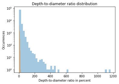
This graph shows Skewed Right distribution. We can see more number of craters for smaller value of the ratio. Which means smaller craters have a smaller depth-to-diameter ratio, while the bigger craters seem to have a bigger depth-to-diameter ratio as well.

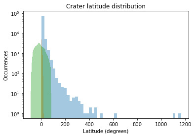
The crater latitude graph also shows the Skewed Right Distribution. We can conclude from the graph that the maximum numbers of craters are located near the Equator.

The Bivariate Graphs are shown below :

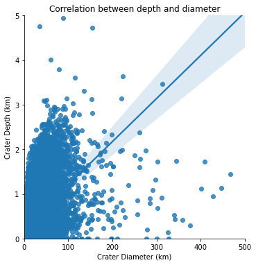
From the graph it is obvious that there is a relationship between these two variables : the greater the diameter, the greater the depth. But the relationship between depth and diameter is somehow weak, as there is a high variability of the scattered plot around the best-fit linear regression.

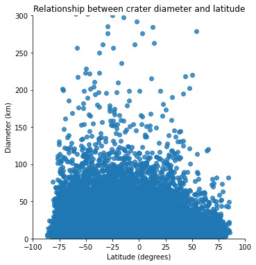
When we plot diameter vs latitude, we see that there is no relationship between these two variables : the location of the impact has apparently no influence on its amplitude.

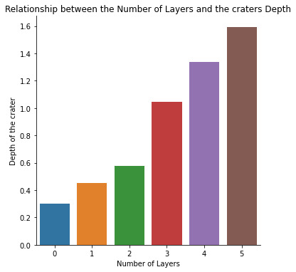
A positive correlation is observed between the number of layers and the depth of the crater. The number of layers of the the crater increases with the increase in the depth of the crater.

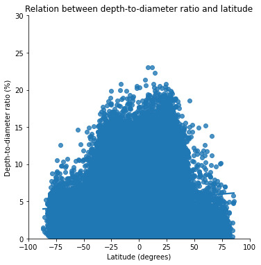
The graph depicting the relationship between the latitude and the depth to diameter ratio. To be honest, I think this is the most interesting plot out of all. 

From this graph it is quite obvious that this ratio is higher for lower latitudes (between -40° and +40° approximately). This correlates with the hard, volcanic terrains which are concentrated around these lower latitudes.

On the other hand, the depth-to-diameter ratio is lower for higher latitudes (below -40° and above +40°). This correlates with the soft, ice-rich terrains which are concentrated around these higher latitudes (closer to the poles).

Which proves my initial hypothesis that the depth-to-diameter ratio depends on the type of terrain where the impact occurs. The harder the terrain, the higher the depth-to-diameter ratio, and the softer the terrain, the lower the depth-to-diameter ratio.

Across the surface of a planetary body, one might expect the ratio of a crater's depth to diameter to be constant since it is a gravity-dominated feature (Melosh, 1989). But, while gravity dominates, terrain properties control this final ratio. Craters are shallower near the equator and deeper near the poles, and this effect persists up to the D <= 30 km range.

Congratulations on making to the end of this article!!

Thank You for your time and patience.

[ryan-data-viz-blog]

Coursera Data Visualization Research Question

As part of the Data Management and Visualization course organized by Wesleyan University on Coursera.org, I’m selecting a set of research data and identifying a question to investigate using the data set.  I’ll be working primarily with two variables in the Mars Crater Study: LATITUDE_CIRCLE_IMAGE and  MORPHOLOGY_EJECTA_1.

I’d like to see if the distribution of different eject morphologies are associated with impact latitude.  Since most of the meteorites that formed these craters would be moving within the plane of the solar system, I’m curious if those that impacted the poles are striking the surface differently.  My central question is whether an association can be seen between the ratio of different ejecta morphologies and the latitude of their impacts.  My hypothesis is that these variables are correlated.

My Code Book

Using the Mars Crater data file (16MB CSV)

LATITUDE_CIRCLE_IMAGE: latitude of the crater’s center point, measured in decimal degrees north

MORPHOLOGY_EJECTA_1:  ejecta morphologies identified at each crater (multiple values are ordered inner-most to outer-most, or top-most to bottom-most, separated by slashes “/”), including the following values

Rd (27,613): radial ejecta morphology (characterized by the lack of a layered ejecta deposit, instead displaying a hummocky continuous ejecta blanket)

SLERS (5,671): single-layer ejecta rampart (sinuous)

SLEPS (5,361): single-layer ejecta pancake (sinuous)

SLEPC (2,846): single-layer ejecta pancake (circular)

DLERS (1,912): double-layer ejecta rampart (sinuous)

SLERC (1,410): single-layer ejecta rampart (circular)

DLEPS (1,131): double-layer ejecta rampart (sinuous)

MLERS (737): multiple-layer ejecta rampart (sinuous)

DLEPC (653): double-layer ejecta pancake (circular)

DLERC (433): double-layer ejecta rampart (circular)

MLEPS (96): multiple-layer ejecta pancake ( sinuous )

SLEPCPd (76): single-layer ejecta pancake (sinuous), pedestal structure

SLEPSPd (53): single-layer ejecta pancake (sinuous), pedestal structure

SLEPd (48): single-layer ejecta, pedestal structure

MLEPC (34): multiple-layer ejecta pancake (circular)

MLERC (33): multiple-layer ejecta rampart (circular)

DLEPCPd (20): double-layer ejecta pancake (circular), pedestal structure

SLERSPd (16): single-layer ejecta rampart (sinuous), pedestal structure

DLEPSPd (13): double-layer ejecta rampart (sinuous), pedestal structure

SLERCPd (11): single-layer ejecta rampart (circular), pedestal structure

DLERCPd (8): double-layer ejecta rampart (circular), pedestal structure

DLERSRd (7): double-layer ejecta rampart (sinuous), radial structure?

DLEPd (6):  double-layer ejecta pedestal structure?

SLERSRd (4): single-layer ejecta rampart (sinuous) , radial structure?

SLEPCRd (3): single-layer ejecta rampart (circular) , radial structure?

DLSPC (1): ???

SLEPSRd (3):  single-layer ejecta pancake (sinuous), radial structure?

Pd (2):  pedestal structure

MLERSRd (1): multiple-layer ejecta rampart (sinuous) , radial structure?

Note: The definitions of some values are unclear, but these are for low-frequency morphologies that will likely be ignored in my analysis.

Literature Review

In the course of reviewing academic literature, I’ve found clear evidence that the total number of craters is greater in lower latitudes and some indications that different morphologies vary independently by latitude.  I searched for the terms “mars ejecta morphology latitude” (not sure why the assignment cares about search terms, though).

For instance, Peter Mouginis-Mark finds that, “Only pancake craters exhibit any pronounced latitudinal variation in their distribution. These craters are almost exclusively located poleward of latitudes 40°N and 40°S.”  Nadine G. Barlow comments that, “... the latidudinal variations seen for rampart crater morphologies correlate well with the proposed latitude-depth relationship for ice and brines across the planet.”