#positivepolicing

[rocio-engineer-blog]

Data Analysis Tools Week 4

Testing a Potential Moderator

Instructions:

Run an ANOVA, Chi-Square Test or correlation coefficient that includes a moderator.

Submission:

Following completion of the steps described above, create a blog entry where you submit syntax used to test moderation (copied and pasted from your program) along with corresponding output and a few sentences of interpretation. 

Criteria:

Your assessment will be based on the evidence you provide that you have completed all of the steps. In all cases, consider that the peer assessing your work is likely not an expert in the field you are analyzing. 

Results:

Continuing with the submussions from previous weeks, I will run an ANOVA analysis that includes a moderator to see:

 -If life expectancy of a country depends on its employ rate

 -If the polity score of the country is a good moderator

CODE:

import numpy

import pandas

import statsmodels.formula.api as smf

import statsmodels.stats.multicomp as multi

import scipy.stats

import seaborn

import matplotlib.pyplot as plt

 # Load gapminder dataset

 data = pandas.read_csv('_7548339a20b4e1d06571333baf47b8df_gapminder.csv', low_memory=False)

 # To avoid having blank data instead of NaN -> Blank data will give you an error.

 data = data.replace(r'^\s*$', numpy.NaN, regex = True)

 # Change all DataFrame column names to Lower-case

 data.columns = map(str.lower, data.columns)

 # Bug fix for display formats to avoid run time errors

 pandas.set_option('display.float_format', lambda x:'%f'%x)

 print('Number of observations (rows)')

print(len(data))

print('Number of Variables (columns)')

print(len(data.columns))

print()

 # Ensure each of these columns are numeric

 data['suicideper100th'] = data['suicideper100th'].apply(pandas.to_numeric, errors='coerce')

data['lifeexpectancy'] = data['lifeexpectancy'].apply(pandas.to_numeric, errors='coerce')

data['urbanrate'] = data['urbanrate'].apply(pandas.to_numeric, errors='coerce')

data['employrate'] = data['employrate'].apply(pandas.to_numeric, errors='coerce')

data['polityscore'] = data['polityscore'].apply(pandas.to_numeric, errors='coerce')

data['internetuserate'] = data['internetuserate'].apply(pandas.to_numeric, errors='coerce')

data['incomeperperson'] = data['incomeperperson'].apply(pandas.to_numeric, errors='coerce')

# Convert a cuantitative variable into a categorical: We will group the polityscore intro 3 cathegories:

def politygroup (row) :

  if row['polityscore'] >= -10 and row['polityscore'] < -3 :

      return 'NegativePolity'

  if row['polityscore'] >= -3 and row['polityscore'] < 4 :

      return 'NeutralPolity'

  if row['polityscore'] >= 4 and row['polityscore'] < 11 :

      return 'PositivePolity'

 sub1['politygroup'] = sub1.apply (lambda row: politygroup (row), axis = 1)

 sub5 = sub1[['politygroup','employrate','suicideper100th','lifeexpectancy']].dropna()

 # Moderator: A third variable that affects the direction and/or strength of the relation between your explanatory or x variable and your response or y variable

 # Testing a moderator with ANOVA:

 Evaluating suicide rate Employ rate groups (Low, Mid and Hihg employ rates), Polity score groups (Negative, Neutral and Positive polity scores):

 sub6 = sub5[(sub5['politygroup'] == 'NegativePolity')]

sub7 = sub5[(sub5['politygroup'] == 'NeutralPolity')]

sub8 = sub5[(sub5['politygroup'] == 'PositivePolity')]

 print('Association between lifeexpectancy and employ rate group (employgroup) for all polity groups')

model99 = smf.ols(formula='lifeexpectancy ~ C(employgroup)', data=sub5)

results99 = model99.fit()

print (results99.summary())

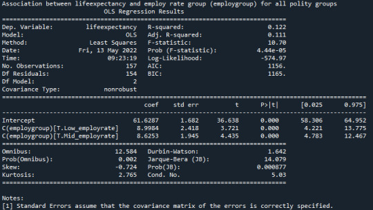
 “P-value = 4.44e-05, the null hypothesis is rejected and can be concluded that the life expectancy is dependent on the employ group.”

 

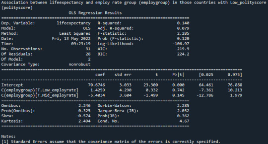
Is there an association between life expectancy and employ rate group (employgroup) in those countries with Low_polityscore (polityscore)?:

 model2 = smf.ols(formula='lifeexpectancy ~ C(employgroup)', data=sub6)

results2 = model2.fit()

print (results2.summary())

 “P-value = 0.120, the null hypothesis cannot be rejected and life expectancy is not dependent on employ rate for countries with low_polityscore”

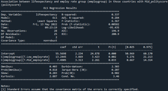
Is there an association between lifeexpectancy and employ rate group (employgroup) in those countries with Mid_polityscore (polityscore)?:

 model3 = smf.ols(formula='lifeexpectancy ~ C(employgroup)', data=sub7)

results3 = model3.fit()

print (results3.summary())

 "P-value = 0.00582, null hypothesis can be rejected and life expectancy is dependent on employ rate for countries with mid_polityscore.”

 

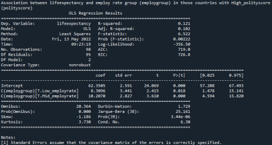
Is there an association between lifeexpectancy and employ rate group (employgroup) in those countries with High_polityscore (polityscore)?:

model4 = smf.ols(formula='lifeexpectancy ~ C(employgroup)', data=sub8)

results4 = model4.fit()

print (results4.summary())

 “P-value = 0.0022 null hypothesis can be rejected and life expectancy is dependent on employ rate for countries with high_polityscore.”

[jorgefuentesdataanalysistools]

Data Analysis Tools: Week 4

By continuing with the previous week homework, we will run an ANOVA analysis that includes a moderator to try to see:

 -Life expectancy of a country depends on its employ rate?

 -Is the polity score of the country a good moderator?

Code and results of running it:

 import numpy

import pandas

import statsmodels.formula.api as smf

import statsmodels.stats.multicomp as multi

import scipy.stats

import seaborn

import matplotlib.pyplot as plt

 # Load gapminder dataset

 data = pandas.read_csv('_7548339a20b4e1d06571333baf47b8df_gapminder.csv', low_memory=False)

 # To avoid having blank data instead of NaN -> If you have blank data the previous line will give you an error.

 data = data.replace(r'^\s*$', numpy.NaN, regex = True)

 # Change all DataFrame column names to Lower-case

 data.columns = map(str.lower, data.columns)

 # Bug fix for display formats to avoid run time errors

 pandas.set_option('display.float_format', lambda x:'%f'%x)

 print('Number of observations (rows)')

print(len(data))

print('Number of Variables (columns)')

print(len(data.columns))

print()

 # Ensure each of these columns are numeric

 data['suicideper100th'] = data['suicideper100th'].apply(pandas.to_numeric, errors='coerce')

data['lifeexpectancy'] = data['lifeexpectancy'].apply(pandas.to_numeric, errors='coerce')

data['urbanrate'] = data['urbanrate'].apply(pandas.to_numeric, errors='coerce')

data['employrate'] = data['employrate'].apply(pandas.to_numeric, errors='coerce')

data['polityscore'] = data['polityscore'].apply(pandas.to_numeric, errors='coerce')

data['internetuserate'] = data['internetuserate'].apply(pandas.to_numeric, errors='coerce')

data['incomeperperson'] = data['incomeperperson'].apply(pandas.to_numeric, errors='coerce')

# Convert a cuantitative variable into a categorical: We will group the polityscore intro 3 cathegories:

def politygroup (row) :

  if row['polityscore'] >= -10 and row['polityscore'] < -3 :

      return 'NegativePolity'

  if row['polityscore'] >= -3 and row['polityscore'] < 4 :

      return 'NeutralPolity'

  if row['polityscore'] >= 4 and row['polityscore'] < 11 :

      return 'PositivePolity'

 sub1['politygroup'] = sub1.apply (lambda row: politygroup (row), axis = 1)

 sub5 = sub1[['politygroup','employrate','suicideper100th','lifeexpectancy']].dropna()

 # Moderator: A third variable that affects the direction and/or strength of the relation between your explanatory or x variable and your response or y variable

 # Testing a moderator in the context of ANOVA:

 Let’s evaluate if suicide rate Employ rate groups (Low, Mid and Hihg employ rates), Polity score groups (Negative, Neutral and Positive polity scores):

 sub6 = sub5[(sub5['politygroup'] == 'NegativePolity')]

sub7 = sub5[(sub5['politygroup'] == 'NeutralPolity')]

sub8 = sub5[(sub5['politygroup'] == 'PositivePolity')]

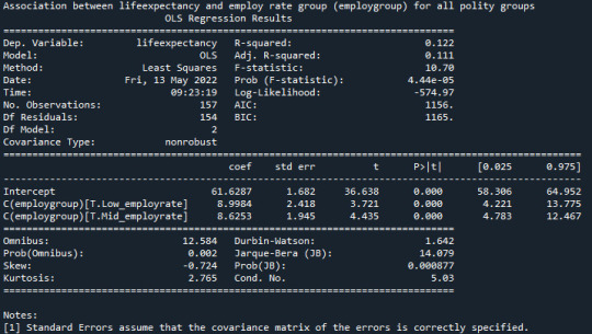
 print('Association between lifeexpectancy and employ rate group (employgroup) for all polity groups')

model99 = smf.ols(formula='lifeexpectancy ~ C(employgroup)', data=sub5)

results99 = model99.fit()

print (results99.summary())

imagen

 “Since p-value = 4.44e-05 so null hypothesis is rejected and we conclude that the life expectancy is dependent on the employ group.”

 Is there an association between lifeexpectancy and employ rate group (employgroup) in those countries with Low_polityscore (polityscore)?:

 model2 = smf.ols(formula='lifeexpectancy ~ C(employgroup)', data=sub6)

results2 = model2.fit()

print (results2.summary())

 “Since p-value = 0.120 so null hypothesis cannot be rejected and life expectancy is not dependent on employ rate for countries with low_polityscore”

 Is there an association between lifeexpectancy and employ rate group (employgroup) in those countries with Mid_polityscore (polityscore)?:

 model3 = smf.ols(formula='lifeexpectancy ~ C(employgroup)', data=sub7)

results3 = model3.fit()

print (results3.summary())

 "Since p-value = 0.00582 null hypothesis can be rejected and life expectancy is dependent on employ rate for countries with mid_polityscore.”

 Is there an association between lifeexpectancy and employ rate group (employgroup) in those countries with High_polityscore (polityscore)?:

model4 = smf.ols(formula='lifeexpectancy ~ C(employgroup)', data=sub8)

results4 = model4.fit()

print (results4.summary())

 “Since p-value = 0.0022 null hypothesis can be rejected and life expectancy is dependent on employ rate for countries with high_polityscore.”

[busydisneymama]

Repost @calgarypolice #bekind #childrensbooks #policehelpingkids #positivepolicing https://www.instagram.com/p/Ch27I15v1cp/?igshid=NGJjMDIxMWI=

[gutssnglory]

☀️Energetic Gifting💧 We are at once influential, impermeable and susceptible to the bioenergy of those around us, and its collective imprint. . Something I always made sure to do on those early morning commutes when I was feeling a little bleh, was to sidle up to the closest person giving off the best vibes, and just bask. . Our being radiates a biofield just as, on a corporeal level, we are capable of measuring the magnetic and electromagnetic fields our cells, tissues, and organs generate. Our biofield, aura, odic force, subtle body.etc., when mechanically measured, was found to consist of various colors (the auric fields), hence frequencies, which correlated to that of the Chakras in conjunction with the color-frequencies expressed in hertz. Today, we are able to measure the bio currents our biofields emit, hitting a frequency between 300 to 2000 nanometers. . Don’t be an energy vampire (EMFs aren’t the only forms of energy we need to protect against), be respectful of people’s personal space, and for all that you receive energetically, gift energetically #workweekhack . #biofield #energeticgifting #auricfield #chakras #odicforce #orgone #subtlebody #auras #electromagnetism #negativepole #positivepole #gutsnglorypodcast #podcasts #intuition #storytelling #gutfeeling #illustration #characterdesign https://www.instagram.com/p/Bv9BuHJg8Vi/?utm_source=ig_tumblr_share&igshid=15jceqtru7uj2

[eugenebutcher]

A personal demo in the hope of flying my 2nd police officer 👮‍♂️ This time it wasn't to be. Maybe straddle throne was ambitious for our 1st move. A close call though! A good guy, had his helmet of ready. Must improve my acro police presentation. Know that I tried 🙏 . . #positivepolicing #YogaPolice #flyingpoliceman #acroyoga (at Whole Foods Market- Picadilly Circus)

[guudlukin]

#thankfulthursday #ayudaalosdemas #teamrubicon #cantonstrong #communitypolicing #blessings #positivepolicing #bikefam #goodmorning #service #familyownedandoperated #children #future #education #equality #opportunity #access #unity #together #humanity #kindness #dogood #art #music #beauty #teaching #learning #lifelessons #l4l #promise

[healthymarc]

Meanwhile back in my home state. Positive policing is going on.

[jorgefuentesdataanalysistools]

Data Analysis Tools: Week 2

By continuing with the previous week homework, we will run 2 chi-square test to try to see:

 -'Do polity score depends on the country group type?'   (PIGS vs EasternEurope vs Rest)

 -For all countries, do the polity score of a country affect its employ rate?

Code and results of running it:

 import numpy

import pandas

import statsmodels.formula.api as smf

import statsmodels.stats.multicomp as multi

import scipy.stats

 # Load gapminder dataset

data = pandas.read_csv('_7548339a20b4e1d06571333baf47b8df_gapminder.csv', low_memory=False)

 # To avoid having blank data instead of NaN -> If you have blank data the previous line will give you an error.

data = data.replace(r'^\s*$', numpy.NaN, regex = True)

 # Change all DataFrame column names to Lower-case

data.columns = map(str.lower, data.columns)

 # Bug fix for display formats to avoid run time errors

pandas.set_option('display.float_format', lambda x:'%f'%x)

 print('Number of observations (rows)')

print(len(data))

print('Number of Variables (columns)')

print(len(data.columns))

print()

 # Ensure each of these columns are numeric

data['suicideper100th'] = data['suicideper100th'].apply(pandas.to_numeric, errors='coerce')

data['lifeexpectancy'] = data['lifeexpectancy'].apply(pandas.to_numeric, errors='coerce')

data['urbanrate'] = data['urbanrate'].apply(pandas.to_numeric, errors='coerce')

data['employrate'] = data['employrate'].apply(pandas.to_numeric, errors='coerce')

data['polityscore'] = data['polityscore'].apply(pandas.to_numeric, errors='coerce')

print(data['polityscore'])

 # Filtering into groups:

print('According to the definition below for Easter European countries and PIGS countries we will create a new column called EuropeEastVsPIGS where:')

print('1 is for Eastern Europe: Bulgaria, Czech Rep., Hungary, Poland, Romania, Russian Federation, Slovakia, Belarus, Moldova and Ukraine')

print('2 is for PiGS countries: Portual, Ireland, Italy, Greece and Spain ')

print()

 def EuropeEastVsPIGS (row) :

  if row['country'] == 'Bulgaria':

      return 1

  if row['country'] == 'Czech Rep.':

      return 1

  if row['country'] == 'Hungary':

      return 1

  if row['country'] == 'Poland':

      return 1

  if row['country'] == 'Romania':

      return 1

  if row['country'] == 'Russia':

      return 1

  if row['country'] == 'Slovak Republic':

      return 1

  if row['country'] == 'Belarus':

      return 1

  if row['country'] == 'Moldova':

      return 1

  if row['country'] == 'Ukraine':

      return 1

  if row['country'] == 'Portugal':

      return 2

  if row['country'] == 'Ireland':

      return 2

  if row['country'] == 'Italy':

      return 2

  if row['country'] == 'Greece':

      return 2

  if row['country'] == 'Spain':

      return 2

 data['EuropeEastVsPIGS'] = data.apply (lambda row: EuropeEastVsPIGS (row), axis = 1)

data['EuropeEastVsPIGS'] = data['EuropeEastVsPIGS'].apply(pandas.to_numeric, errors='coerce')

 # Replace NaN with 99 to use as others

data['EuropeEastVsPIGS'].fillna(99, inplace=True)

 sub1 = data.copy()

 # Chi Square test of independence: when we have a categorical explanatory variabale and a categorial response variable:

 -'Do polity score depends on the country group type?'

# Convert a cuantitative variable into a categorical: We will group the polityscore intro 4 cathegories:

 def politygroup (row) :

  if row['polityscore'] >= -10 and row['polityscore'] < -3 :

      return 'NegativePolity'

  if row['polityscore'] >= -3 and row['polityscore'] < 4 :

      return 'NeutralPolity'

  if row['polityscore'] >= 4 and row['polityscore'] < 11 :

      return 'PositivePolity'

 sub1['politygroup'] = sub1.apply (lambda row: politygroup (row), axis = 1)

 sub4 = sub1[['EuropeEastVsPIGS','politygroup']].dropna()

 # Contingency table of observed counts

ct1 = pandas.crosstab(sub4['EuropeEastVsPIGS'], sub4['politygroup'])

print(ct1)    

print()

 # Column percentages

colsum = ct1.sum(axis=0)

colpct = ct1/colsum

print(colpct)

print()  

 # Chi-square

print('Chi-Square value, p-value, expected counts')

cs1 = scipy.stats.chi2_contingency(ct1)

print(cs1)

print()

 Since the p-value = 0.134 we cannot reject the null hypothesis and hence there are no diferences between the groups defined. The results are based on having a "Rest of the world" group that has a lot of countries on it.

 -For all countries, do the polity score of a country affect its employ rate?

 # Another example of the use of Chi-Square:

print('For all countries, do polity score group affect the employ rate of a country?')

 sub5 = sub1[['politygroup','employrate']].dropna()

 # Group into 3 categories the employ rate of countries

# Change NaN values to 0 to get max value in employ rate column

sub6 = sub5.copy()

sub6.fillna(0, inplace=True)

sub6_maxer = sub6['employrate'].max()

 sub7 = sub5.copy()

sub7.fillna(999, inplace=True)

sub7_min = sub7['employrate'].min()

 employlow = 0.33*(sub6_maxer - sub7_min) + sub7_min

employhigh = 0.66*(sub6_maxer - sub7_min) + sub7_min

 def employgroup (row) :

  if row['employrate'] >= sub7_min and row['employrate'] < employlow :

      return 'Low_employrate'

  if row['employrate'] >= employlow and row['employrate'] < employhigh :

      return 'Mid_employrate'

  if row['employrate'] >= employhigh and row['employrate'] <= sub6_maxer :

      return 'High_employrate'

 sub5['employgroup'] = sub1.apply (lambda row: employgroup (row), axis = 1)

 # Contingency table of observed counts

ct2 = pandas.crosstab(sub5['politygroup'], sub5['employgroup'])

print(ct2)    

print()

 # Column percentages

colsum2 = ct2.sum(axis=0)

colpct2 = ct2/colsum2

print(colpct2)

print()  

 # Chi-square

print('Chi-Square value, p-value, expected counts')

cs2 = scipy.stats.chi2_contingency(ct2)

print(cs2)

print()

 Since the p-value = 0.0059, null hypothesis is rejected and we can conclude that the employ rate depends on the polityscore of the country. We know they are not equal but we dont know which ones are equals and which are not. To know this a post-hoc test is needed.

 # If we reject the null hypothesis, we need to perform comparisons for each pair of groups.

# To appropiate protect against type 1 error in the contxt of a chi-squared test, we wil use the post-hoc called "Bonferroni Adjustment"

 # For that we will make 2 groups comparisons:

 # For 1st pair of groups:

 recode3 = {'High_employrate':'High_employrate' , 'Mid_employrate':'Mid_employrate' }

sub5['Comp1vs2'] = sub5['employgroup'].map(recode3)

 # Contingency table of observed counts

ct3 = pandas.crosstab(sub5['politygroup'], sub5['Comp1vs2'])

print(ct3)    

print()

 # Column percentages

colsum3 = ct3.sum(axis=0)

colpct3 = ct3/colsum3

print(colpct3)

print()  

 # Chi-square

print('Chi-Square value, p-value, expected counts')

cs3 = scipy.stats.chi2_contingency(ct3)

print(cs3)

 Since the p-value = 0.00086, null hypothesis is rejected and we can conclude that there is a significant difference between this 2 groups. High_employrate group is different from Mid_employrate group.

 # For 2nd pair of groups:

 recode4 = {'High_employrate':'High_employrate' , 'Low_employrate':'Low_employrate' }

sub5['Comp1vs3'] = sub5['employgroup'].map(recode4)

 # Contingency table of observed counts

ct4 = pandas.crosstab(sub5['politygroup'], sub5['Comp1vs3'])

print(ct4)    

print()

 # Column percentages

colsum4 = ct4.sum(axis=0)

colpct4 = ct4/colsum4

print(colpct4)

print()  

 # Chi-square

print('Chi-Square value, p-value, expected counts')

cs4 = scipy.stats.chi2_contingency(ct4)

print(cs4)

 Since the p-value = 0.29063, null hypothesis cannot be rejected and we can conclude that there is no significant difference between this 2 groups. High_employrate group is simmilar to low_employ rate group.

 # For 3rd pair of groups:

 recode5 = {'Low_employrate':'Low_employrate' , 'Mid_employrate':'Mid_employrate' }

sub5['Comp2vs3'] = sub5['employgroup'].map(recode5)

 # Contingency table of observed counts

ct5 = pandas.crosstab(sub5['politygroup'], sub5['Comp2vs3'])

print(ct5)    

print()

 # Column percentages

colsum5 = ct5.sum(axis=0)

colpct5 = ct5/colsum5

print(colpct5)

print()  

 # Chi-square

print('Chi-Square value, p-value, expected counts')

cs5 = scipy.stats.chi2_contingency(ct5)

print(cs5)

imagen

 Since the p-value = 0.24568, null hypothesis cannot be rejected and we can conclude that there is no significant difference between this 2 groups. Mid_employrate group is simmilar to low_employ rate group.

[rocio-engineer-blog]

Week 4: Creating graphs for your data

By continuing with the previous week homework, we will run an ANOVA analysis that includes a moderator to try to see:

-Life expectancy of a country depends on its employ rate?

-Is the polity score of the country a good moderator?

Code and results of running it:

# -*- coding: utf-8 -*- """ Created on Tue Apr 19 16:42:34 202

"""

import numpy import pandas import statsmodels.formula.api as smf import statsmodels.stats.multicomp as multi import scipy.stats import seaborn import matplotlib.pyplot as plt

# Load gapminder dataset

data = pandas.read_csv('_7548339a20b4e1d06571333baf47b8df_gapminder.csv', low_memory=False)

# To avoid having blank data instead of NaN -> If you have blank data the previous line will give you an error.

data = data.replace(r'^\s*$', numpy.NaN, regex = True)

# Change all DataFrame column names to Lower-case

data.columns = map(str.lower, data.columns)

# Bug fix for display formats to avoid run time errors

pandas.set_option('display.float_format', lambda x:'%f'%x)

print('Number of observations (rows)') print(len(data)) print('Number of Variables (columns)') print(len(data.columns)) print()

# Ensure each of these columns are numeric

data['suicideper100th'] = data['suicideper100th'].apply(pandas.to_numeric, errors='coerce') data['lifeexpectancy'] = data['lifeexpectancy'].apply(pandas.to_numeric, errors='coerce') data['urbanrate'] = data['urbanrate'].apply(pandas.to_numeric, errors='coerce') data['employrate'] = data['employrate'].apply(pandas.to_numeric, errors='coerce') data['polityscore'] = data['polityscore'].apply(pandas.to_numeric, errors='coerce') data['internetuserate'] = data['internetuserate'].apply(pandas.to_numeric, errors='coerce') data['incomeperperson'] = data['incomeperperson'].apply(pandas.to_numeric, errors='coerce')

# Convert a cuantitative variable into a categorical: We will group the polityscore intro 3 cathegories:

def politygroup (row) :    if row['polityscore'] >= -10 and row['polityscore'] < -3 :        return 'NegativePolity'    if row['polityscore'] >= -3 and row['polityscore'] < 4 :        return 'NeutralPolity'    if row['polityscore'] >= 4 and row['polityscore'] < 11 :        return 'PositivePolity'

sub1['politygroup'] = sub1.apply (lambda row: politygroup (row), axis = 1)

sub5 = sub1[['politygroup','employrate','suicideper100th','lifeexpectancy']].dropna()

# Moderator: A third variable that affects the direction and/or strength of the relation between your explanatory or x variable and your response or y variable

# Testing a moderator in the context of ANOVA:

Let’s evaluate if suicide rate Employ rate groups (Low, Mid and Hihg employ rates), Polity score groups (Negative, Neutral and Positive polity scores):

sub6 = sub5[(sub5['politygroup'] == 'NegativePolity')] sub7 = sub5[(sub5['politygroup'] == 'NeutralPolity')] sub8 = sub5[(sub5['politygroup'] == 'PositivePolity')]

print('Association between lifeexpectancy and employ rate group (employgroup) for all polity groups') model99 = smf.ols(formula='lifeexpectancy ~ C(employgroup)', data=sub5) results99 = model99.fit() print (results99.summary())

“Since p-value = 4.44e-05 so null hypothesis is rejected and we conclude that the life expectancy is dependent on the employ group.”

Is there an association between lifeexpectancy and employ rate group (employgroup) in those countries with Low_polityscore (polityscore)?:

model2 = smf.ols(formula='lifeexpectancy ~ C(employgroup)', data=sub6) results2 = model2.fit() print (results2.summary())

“Since p-value = 0.120 so null hypothesis cannot be rejected and life expectancy is not dependent on employ rate for countries with low_polityscore”

Is there an association between lifeexpectancy and employ rate group (employgroup) in those countries with Mid_polityscore (polityscore)?:

model3 = smf.ols(formula='lifeexpectancy ~ C(employgroup)', data=sub7) results3 = model3.fit() print (results3.summary())

"Since p-value = 0.00582 null hypothesis can be rejected and life expectancy is dependent on employ rate for countries with mid_polityscore.”

Is there an association between lifeexpectancy and employ rate group (employgroup) in those countries with High_polityscore (polityscore)?: model4 = smf.ols(formula='lifeexpectancy ~ C(employgroup)', data=sub8) results4 = model4.fit() print (results4.summary())

“Since p-value = 0.0022 null hypothesis can be rejected and life expectancy is dependent on employ rate for countries with high_polityscore.”