#setting date format for Category Axis Value
Explore tagged Tumblr posts
Visit Tumblr Blog
Explore Tumblr blogs with no restrictions, modern design and the best experience.
Last Seen Tumblr Blogs


Fun Fact
Tumblr’s website traffic is steadily declining.
Text
.NET Core Support, Setting Precision of Data in Chart Data Labels using .NET
What's New in this Release?
Aspose team is happy to share the announcement of Aspose.Slides for .NET 18.6. In this release we have improved the chart support by adding new features along with resolution of other issues. There are some important new features part of this release, such as .NET Standard/.NET Core support, Setting Precision of Data in chart Data Labels, Support for setting date format for Category Axis Value, Support for setting rotation angle for chart axis title, Switch Data over axis, Setting Chart Marker Options, support of setting Position Axis in Category or Value Axis, Support for showing Display Unit label on Chart value axis and Support for Bubble chart Size scaling. There are some important enhancements and bug fixes also part of this release, such as improvement in quality of generated PDF, The WMF image is corrupted in PDF output, Chart rendering issues in exported PDF, PPTX to PDF – space difference between text and line, When PPTX is converted to PDF, the vertical graphs lines are different, Circles in the output PDF don’t match the source presentation, The chart horizontal axis is corrupted in PDF output, Font styles change to italic when saving presentation as HTML, JpegQuality setting not works when saving PPTX with JPEG image as PDF, Setting chart data value in chart worksheet does not refresh chart and many more. This list of new, improved and bug fixes in this release are given below
.NET Standard/.NET Core support
Support for setting precision of data in chart data label Featur
Support for setting the date format for Category Axis Value
Support for setting rotation angle for chart axis title
Support for switch Row/Column for chart data
Setting the chart marker options on data points level
Support of setting Position Axis in Category or Value Axis
Support for showing Display Unit label on Chart value axis
Support for setting markers and its properties for particular chart series point
Getting Series Data Point color from Theme
Support for Bubble chart Size scaling
Setting Series Overlap for Clustered Bar Chart
Support for managing visibility of data labels located outside of plot area
Improve slide graph quality
Low quality PDF generated
The WMF image is corrupted in PDF output
When PPTX is converted to PDF, vertical axis of the graph contains additional items.
PPTX to PDF - space difference between text and line
When PPTX is converted to PDF, the vertical graphs lines are differen
Some spacing is lost in the output PDF
Circles in the output PDF don't match the source presentation
The chart horizontal axis is corrupted in PDF output
Font styles change to italic when saving presentation as HTML
JpegQuality setting not works when saving PPTX with JPEG image as PDF
Setting chart data value in chart worksheet does not refresh chart
Chart data not updating
The animation synchronization is lost in the output presentation
NullReference exception is thrown on loading presentation
PPT to PPTX conversion result in corrupt presentation due to WordArt text present in slide
Custom Marker image failed to rendered in generated PDF
Shadow effects on text are lost when saving presentation using Aspose.Slides
Paragraph text is not splitted in portions on changing the shadow effect on portion text
WordArt is improperly rendered in generated PDF
Improper vertical axis rendering in generated PNG
Export to PPTX works but PPT fails
Exception on presentation load
XmlException on loading the presentation
Font size changes after saving
Background change color after saving
PPTX to PDF not properly converted
Charts are improperly rendered in generated PDF
Chart changes after cloning
Layout changed while converting PPTX to PDF
Language changed when converting PPTX to PDF
Low quality images generated from presentation
The axis major unit has been changed in generated PNG
Chart title differs from expected
PPTXReadException on loading presentation
Repair message in saved file
NullPointer Exception on loading presentation
PPTXReadException on loading presentation
System.Exception on loading presentation
ODP to PPTX not properly converted
Content moved in generated HTML
PPTX not properly converted to PPT
Saved PPT presentation requires repairing in PowerPoint
Application Hangs while saving PPTX
Conversion process never ends
Argument Exception is thrown in Box&Whisker chart has only 2 categories
etting RawFrame property has no effect for SmartArtShape
Overflow exception on saving if chart data point has blank value
No format validation for images resource
Other most recent bug fixes are also included in this release
Newly added documentation pages and articles
Some new tips and articles have now been added into Aspose.Slides for Java documentation that may guide users briefly how to use Aspose.Slides for performing different tasks like the followings.
Setting Chart Marker Options
Setting Precision of Data in chart Data Labels
Overview: Aspose.Slides for .NET
Aspose.Slides is a .NET component to read, write and modify a PowerPoint document without using MS PowerPoint. PowerPoint versions from 97-2007 and all three PowerPoint formats: PPT, POT, PPS are also supported. Now users can create, access, copy, clone, edit and delete slides in their presentations. Other features include saving PowerPoint slides into PDF, adding & modifying audio & video frames, using shapes like rectangles or ellipses and saving presentations in SVG format, streams or images.
More about Aspose.Slides for .NET
Homepage of Aspose.Slides for .NET
Downlaod of Aspose.Slides for .NET
Online documentation of Aspose.Slides for .NET
#.NET Core support#set Chart Marker Options#setting date format for Category Axis Value#set Precision of Data in chart Labels#rotation angle for chart axis title#.NET PowerPoint API
0 notes
Text
Video editing - Wikipedia
Video Edit Magic
It enables us to orientate three-dimensionally in space. Avoiding so-called axis jumps is also part of dealing with space in assembly. The camera jumps over the imaginary image axis so that two people no longer face each other on the right and left, but suddenly without movement on the left and right). You can do all of this without any previous video editing skills. The tool we recommend for this purpose, and which has been used by millions of users around the world, is Clipchamp. If you want to crop or split the video at a specific point, you can simply enter the time in the field next to the crop button. Click the "X" above an area if you want to undo the step. Like many other modern arts, montage derived its early constitutive power from the nineteenth century. Flaubert's literary realism, whose words have wrested metaphorical meaning from the inconspicuous detail, finds its reference in the film montage. In addition, the quality of the encoded images has been significantly improved in the GIF formats. This has become possible thanks to the dithering effect. Murch explicitly understands his checklist (hereinafter simplified under point 4) as a priority list. If you are faced with the decision to choose emotion or rhythm, you should rely on the overriding criterion of emotion. If you are unsure whether storytelling or rhythm is more important, you should rely on storytelling, and so on. Video Edit Magic makes films in MPEG formats that are used when you create DVDs.
WMV format files - image and sound loss in defective files; sound defects in multiple scenes; no notification if a YouTube category is not supported; dpi support issues; incorrect decoding of interlaced video.
Next, click Upload and Share to start uploading your video .
Program crash when working with DivX files. Program crash when activating certain firewall settings in the system. Error messages when writing to a network drive. Centering of objects on the scene. li> ul> It allows changing the semi-transparency of the image in certain areas of the object and applying effects to its certain areas. WMV format files - image and sound loss in defective files; sound defects in multiple scenes; no notification if a YouTube category is not supported; problems with dpi support; incorrect decoding of interlaced video. 'Pack project' feature added with an option to save and transfer a project file and all of its output (raw) resources to another computer. Added basic effects window with main adjustment effects, RGB and YUV curves, and quick rotation tools available in a control panel. This also makes it clear why the film and video montage, in contrast to the so-called editing (or editing) as a pure next page Linking and "cleaning up" of the footage, the value of the film cut should be far superior. The user interface is simpler and more uniform. The values can be scaled on a value scale. This makes the setting of the values more precise. All settings of the app are now in one central place.
Online film cost calculator: image films, web videos, dates and file sizes

Editing and assembly also have their past. This can be shown. It goes far beyond the history of digital image processing, computers, edit files and software for editing. With Imaging Edge Mobile, you can transfer videos that you want to edit with the Movie Edit add-on from the camera to your smartphone.
1 note
·
View note
Text
Pandas
To import Pandas; import pandas as pd
To create a dataframe from a csv: fd = pd.read_csv("title.csv")
To see the first 5 rows of a dataframe: df.head()
To get the number of rows and columns: df.shape
To get the names of the columns: df.columns
To see NaN (not a number) values (where True = NaN): df.isna()
To see the last 5 rows of a dataframe: df.tail()
To create a clean dataframe without rows with NaN: clean_df = df.dropna()
To access a particular column by name: clean_df['Starting Median Salary']
To find the highest value in a column: clean_df['Starting Median Salary'].max()
To get the row number or index of that value: clean_df['Starting Median Salary'].idxmax()
To get the value from another column at that index: clean_df['Undergraduate Major'].loc[43] OR clean_df['Undergraduate Major'][43]
To get the entire row at a given index: clean_df.loc[43]
To get the difference between two columns:
clean_df['Mid-Career 90th Percentile Salary'] - clean_df['Mid-Career 10th Percentile Salary'] OR
clean_df['Mid-Career 90th Percentile Salary'].subtract(clean_df['Mid-Career 10th Percentile Salary'])
To insert this as a new column;
spread_col = clean_df['Mid-Career 90th Percentile Salary'] - clean_df['Mid-Career 10th Percentile Salary']
clean_df.insert(1, 'Spread', spread_col)
clean_df.head()
To create a new table sorted by a column: low_risk = clean_df.sort_values('Spread')
To only display two columns: low_risk[['Undergraduate Major', 'Spread']].head()
To see how many of each type you have:
clean_df.groupby('Group').sum()
To count how many you have by of each category: clean_df.groupby('Group').count()
To round to two decimal places:
pd.options.display.float_format = '{:,.2f}'.format
To get the averages for each category:
clean_df.groupby('Group').mean()
To rename columns:
df = pd.read_csv('QueryResults.csv', names=['DATE', 'TAG', 'POSTS'], header=0)
To get the sum of entries:
df.groupby("TAG").sum()
To count how many entries there are:
df.groupby("TAG").count()
To select an individual cell:
df['DATE'][1]
or df.DATE[1]
To inspect the datatype:
type(df["DATE"][1])
To convert a string into a datetime:
df.DATE = pd.to_datetime(df.DATE)
To pivot a dataframe:
reshaped_df = df.pivot(index='DATE', columns='TAG', values='POSTS')
To replace NaN with zeros:
reshaped_df.fillna(0, inplace=True) or
reshaped_df = reshaped_df.fillna(0)
To check there aren't any NaN values left:
reshaped_df.isna().values.any()
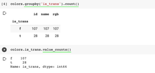
To count how many of each type there is:
colors.groupby("is_trans").count() or
colors.is_trans.value_counts()
To find all the entries with a certain value (to filter by a condition):
sets[sets['year'] == 1949]
To aggregate data:
themes_by_year = sets.groupby('year').agg({'theme_id': pd.Series.nunique})
Note, the .agg() method takes a dictionary as an argument. In this dictionary, we specify which operation we'd like to apply to each column. In our case, we just want to calculate the number of unique entries in the theme_id column by using our old friend, the .nunique() method.
To rename columns:
themes_by_year.rename(columns = {'theme_id': 'nr_themes'}, inplace= True)
To plot:
plt.plot(themes_by_year.index[:-2], themes_by_year.nr_themes[:-2])
To plot two lines with two axis:
ax1 = plt.gca() # get current axes
ax2 = ax1.twinx() #allows them to share the same x-axis
ax1.plot(themes_by_year.index[:-2], themes_by_year.nr_themes[:-2])
ax2.plot(sets_by_year.index[:-2], sets_by_year.set_num[:-2])
ax1.set_xlabel("Year")
ax1.set_ylabel("Number of Sets", color="green")
ax2.set_ylabel("Number of Themes", color="blue")
To get the average number of parts per year:
parts_per_set = sets.groupby('year').agg({'num_parts': pd.Series.mean})
To change daily data to monthly data:
df_btc_monthly.head()
0 notes
Text
SOLUTION AT Academic Writers Bay Please view explanation and answer below.Hey, buddy. 😄 I want to notify you about the progress of the homework. I have already completed questions number 1: GDP for Saudi Arabia and number 2: Memo / Policy. I’ve chosen a policy for overtime. I followed a template to learn the format of a memo. BUT I revised and changed it to prevent plagiarism. Kindly check it and feel free to ask if it is already good for you. Thank you. 😄Outline•Answer #1: Gross Domestic Product (GDP) Per Capita for Saudi Arabia•Answer #2 Memos for Employees (Overtime Policy)Answer for Question No. 1: Gross Domestic Product (GDP) Per Capita for Saudi ArabiaThe data gathering, illustration, analysis, and interpretation of statistics observations arecalled statistics. Statisticians and even business writers may represent statistical data in quite afew ways, including tables, pie charts, histograms, and, notably, bar graphs (BJYU, 2020).Bar graphs are also commonly known as bar charts. Bar charts are the most effectivemethods to demonstrate and compare data series over time (SmartWork, 2020).As we said, bar Graphs or bar charts are typically used to demonstrate and compare data.A bar graph illustrates data using a vertical or horizontal square bar, wherein the length of thebars signifies how small or huge the measured data is. The longer the bar means, the greater thevalue of data is.The business writer utilized a bar graph to effectively demonstrate Gross DomesticProduct (GDP) Per Capita for Saudi Arabia.It can be seen that there are a series of data. In the x-axis, we can see the Q refers to thequarte, and 2020 and 2021 refer to the year. At the same time, the y axis refers to the value ofGDP for Saudi Arabia.At first sight, you can quickly determine the highest GDP, which is Q2 2021, and thesmallest GDP, which is Q2 2020. Through the length of the bars, we can quickly identify thedifferences in data without looking into the numbers. It is practical, especially when you arepresenting the data with different measurements and variables. You can easily compare anddetermine their difference just by looking at the bars.According to Smart Draw (2020), bar graphs effectively compare a series of data amongvarious categories just by looking at them. Second, bar graphs are used to demonstrate therelationship between the x-axis and y-axis. And lastly, it shows the drastic changes in values ofthe data over time. These attributes are evident in the bar graph for demonstrating GrossDomestic Product (GDP) Per Capita for Saudi Arabia. Thus, the business writer chose and usedthis particular visual aid.Answer for Question No. 2:Memos for Employees (Overtime Policy)Note: Kindly see the Policy below.TAI MEDICAL HOSPITALPOLICIES AND PROCEDURESEffective Date: December 2, 2021Date Deleted/Replaced: November 17, 2021Review Responsibility: Human Resources and Senior Director-ManagerOvertime PolicyPURPOSE & POLICY STATEMENT:To set domain and parameters for overtime payment.A.Employers will pay Non-exempt employees 1.5 times the regular wage if theywork more than 40 hours a week. To determine or justify the qualifications of theemployees for overwork pay, they should consult with their manager.B.Employers would pay Non-exempt employees with regular working hours (8hours or less per day) 1.5 times the standard hourly wage in a week if they worked morethan 8.25 hours on the working day or 40 hours later. If an employee is eligible to workovertime, there are additional 1.5 times the regular hourly wage after the regular eighthour-work.Example: Employees who work 8.25 hours a day receive an 8.25-hour regular salary.Employees who work 8.5 hours a day receive 8 hours of a regular salary and 0.5 hours ofovertime.C.Non-exempt employees with flexible schedules will receive overtime afterworking more than 15 minutes per day on their budget, or 40 hours per week.Example: Employees need to work on shifts of 3-12 hours each week. Employees whowork 12.25 hours a day receive a regular salary of 12.
25 hours. Employees who work 12.5hours a day receive 12 hours of a regular salary and 0.5 hours of overtime. If an employeespends additional hours in the remaining work week, resulting in more than 40 hours ofwork in this workweek, employers will pay overtime pay for all overtime work above 40hours.D.Staff and employees are prohibited from doing overtime work without the prior approvalof their senior director or department head. Employees will receive overtime pay for allovertime but should be disciplined through termination if overtime work isunauthorized. If the employee illegally does overtime work, the employee’ssupervisor/manager should:1. Speak with the employee regarding the policies, authorization, and permissionto work overtime.2. Record the discussion with the employee.3. Maintain documentation in the manager’s employee file.E.Employers will pay employees who work less than 8 hours per workday or 40hours per workweek at their usual hourly rate for overtime up to 8 hours. Hours workedmore than 8.25 hours in a workday or more than 40 hours in a workweek will be paid atthe appropriate overtime rate.F.In calculating appropriate overtime fees, an employee’s usual pay rate will includeall pay differentials to determine overtime conditions for working hours exceeding 8.25hours in a working day. All hours worked by non-exempt employees immediately beforeor after their regular shift are considered worked on the same workday as their regularshift.G.To identify daily overtime eligibility, the time an employee works outside of theirstandard shift is not immediately before or after and falls at the end of the day. Employeesshall work during the business day on which the change begins.H.To determine if an employee is entitled to overtime pay, all hours worked in aworkweek are counted. Subsidized time for jury duty will also count toward hours workedto determine overtime eligibility for several hours worked after 40 hours in a workingweek. Sickness pay, personal time, and bereavement pay will not be considered hoursworked in determining eligibility for overtime premiums.I.Compensation for daily and weekly overtime cannot be copied or duplicated.Subsequently, staffs and employees are unauthorized for daily and weekly overtime pay.Only an overtime premium will apply.J.Employees must be prohibited from working more than 16 consecutive hours at atime. If an employee works 16 hours in a row, he will not work another shift without atleast 10 hours of rest or shifts. Employees cannot work more than 56 hours per week andmore than seven consecutive days without at least 24 hours of free time.K.L.Compensatory leave in place of overtime pay is never allowed.Any changes and exceptions to this policy must be reviewed and approved by the SeniorDirector-Manager of Tai Medical Hospital.SCOPE:This policy applies to all personnel of Thai Medical Hospital. However, withinside the occasionof any conflict among this coverage and the provisions of the collective bargaining settlement,the relevant provisions of the collective bargaining settlement shall prevail.RESPONSIBILITY:A.Employers and managers, along with the Human Resources department, are responsiblefor these employees’ compliance with this policy.B.Employers and managers are liable for informing staff and employees about the changeswithin the administration and the policy itself.C.Employees must do accurately report all working time, and it includes overtime workinghours.PROCEDURE:A. To make sure ongoing powerful operations, personnel must only work reasonable overtimehours. Whenever possible, managers will equitably distribute extra time to the variouspersonnel withinside the affected department(s).B. Department Heads will assign extra time, giving enough notice and information every timefeasible. However, emergencies and the unexpected situation might cancel the notice.C.In the case of emergencies, personnel can be required to work over the hoursindexed in Section K above.D. For employees who work within 11 p.
m. to 7 a.m shifts at night time, the time adjustmentsbecause of daytime savings time willreceive 7 hours payment during the spring season and 8 hours for a regular fee plus theovertime payment during the fall season.MONITORING:Individual managers and Human Resources are liable for monitoring, evaluating, and ensuringcompliance with this policy.APPROVAL:Human Resources Senior ManagerREVIEW/REVISED:Date 11/19/21ReferencesBYJU. (2020, December 7). Bar graph. BYJUS. https://byjus.com/maths/bar-graph/Oregon State University. (2020, September 9). Responsible employees and reporting incidents ofsexual misconduct or discrimination. University Policies andStandards. https://policy.oregonstate.edu/UPSM/05-005_responsible_employeesSmart Work. (2020). What is a Bar Graph Used For. https://www.smartdraw.com/bargraph/#:~:text=Bar graphs are an extremely effective visual to,several different styles of bar graphs to considerOutline•Answer #1: Gross Domestic Product (GDP) Per Capita for Saudi Arabia•Answer #2 Memos for Employees (Overtime Policy)Answer f… CLICK HERE TO GET A PROFESSIONAL WRITER TO WORK ON THIS PAPER AND OTHER SIMILAR PAPERS CLICK THE BUTTON TO MAKE YOUR ORDER
0 notes
Text
Data Analyst 2v2
1) Program: Gapminder2v2.py
import pandas import numpy import scipy.stats import statsmodels.formula.api as sf_api import seaborn import matplotlib.pyplot as plt
""" any additional libraries would be imported here """
""" Set PANDAS to show all columns in DataFrame """ pandas.set_option('display.max_columns', None)
"""Set PANDAS to show all rows in DataFrame """ pandas.set_option('display.max_rows', None)
""" bug fix for display formats to avoid run time errors """ pandas.set_option('display.float_format', lambda x:'%f'%x)
""" read in csv file """ data = pandas.read_csv('gapminder.csv', low_memory=False) data = data.replace(r'^\s*$', numpy.NaN, regex=True)
""" checking the format of your variables """ data['country'].dtype
""" setting variables you will be working with to numeric """ data['employrate'] = pandas.to_numeric(data['employrate'], errors='coerce') data['internetuserate'] = pandas.to_numeric(data['internetuserate'], errors='coerce') data['lifeexpectancy'] = pandas.to_numeric(data['lifeexpectancy'], errors='coerce')
""" subset of employrate less than 76 percent, internetuserate between 25 - 75 percent and lifeexpectancy between 50 - 75 years """ sub1=data[(data['employrate'] <= 75) & (data['lifeexpectancy'] > 50) \ & (data['lifeexpectancy'] <= 75) & (data['internetuserate'] > 50) \ & (data['internetuserate'] <= 75)]
""" make a copy of subset data 1 """ sub2=sub1.copy()
""" recoding - replace NaN to 0 and recoding to interger """ sub2['employrate'].fillna(0, inplace=True) sub2['internetuserate'].fillna(0, inplace=True) sub2['lifeexpectancy'].fillna(0, inplace=True) sub2['employrate']=sub1['employrate'].astype(int) sub2['internetuserate']=sub1['internetuserate'].astype(int) sub2['lifeexpectancy']=sub1['lifeexpectancy'].astype(int)
""" recode quantitative variable to categorical to practice chi-square """ sub2['employrate'].astype('category') sub2['internetuserate'].astype('category')
""" use ols function for F-statistic and associated p-value """ model_a = sf_api.ols(formula='employrate ~ C(internetuserate)', data=sub2).fit() print(model_a.summary())
sub3=sub2[['employrate', 'internetuserate']].dropna().astype(int)
""" contingency table of observed counts """ print("contingency table of observed counts") oc=pandas.crosstab(sub3['employrate'], sub3['internetuserate']) print(oc)
""" column percentages """ colpct=oc/oc.sum(axis=0) print("column percentages of contingency table") print(colpct)
""" chi-square test of independence """ print("chi-square, p value, expected counts") cs=scipy.stats.chi2_contingency(oc) print(cs)
2) Output: Chi-Square Test of Independence
OLS Regression Results ============================================================================== Dep. Variable: employrate R-squared: 1.000 Model: OLS Adj. R-squared: nan Method: Least Squares F-statistic: nan Date: Fri, 26 Feb 2021 Prob (F-statistic): nan Time: 18:03:05 Log-Likelihood: 219.29 No. Observations: 7 AIC: -424.6 Df Residuals: 0 BIC: -425.0 Df Model: 6 Covariance Type: nonrobust ============================================================================================ coef std err t P>|t| [0.025 0.975] -------------------------------------------------------------------------------------------- Intercept 34.0000 inf 0 nan nan nan C(internetuserate)[T.56] 26.0000 inf 0 nan nan nan C(internetuserate)[T.61] 16.0000 inf 0 nan nan nan C(internetuserate)[T.62] 19.0000 inf 0 nan nan nan C(internetuserate)[T.65] 13.0000 inf 0 nan nan nan C(internetuserate)[T.71] 22.0000 inf 0 nan nan nan C(internetuserate)[T.74] 22.0000 inf 0 nan nan nan ============================================================================== Omnibus: nan Durbin-Watson: 1.400 Prob(Omnibus): nan Jarque-Bera (JB): 0.749 Skew: -0.272 Prob(JB): 0.688 Kurtosis: 1.493 Cond. No. 7.87 ==============================================================================
Notes: [1] Standard Errors assume that the covariance matrix of the errors is correctly specified. contingency table of observed counts internetuserate 51 56 61 62 65 71 74 employrate 34 1 0 0 0 0 0 0 47 0 0 0 0 1 0 0 50 0 0 1 0 0 0 0 53 0 0 0 1 0 0 0 56 0 0 0 0 0 1 1 60 0 1 0 0 0 0 0 column percentages of contingency table internetuserate 51 56 61 62 65 71 74 employrate 34 1.000000 0.000000 0.000000 0.000000 0.000000 0.000000 0.000000 47 0.000000 0.000000 0.000000 0.000000 1.000000 0.000000 0.000000 50 0.000000 0.000000 1.000000 0.000000 0.000000 0.000000 0.000000 53 0.000000 0.000000 0.000000 1.000000 0.000000 0.000000 0.000000 56 0.000000 0.000000 0.000000 0.000000 0.000000 1.000000 1.000000 60 0.000000 1.000000 0.000000 0.000000 0.000000 0.000000 0.000000 chi-square, p value, expected counts (35.000000000000014, 0.24264043734973734, 30, array([ [0.14285714, 0.14285714, 0.14285714, 0.14285714, 0.14285714, 0.14285714, 0.14285714], [0.14285714, 0.14285714, 0.14285714, 0.14285714, 0.14285714, 0.14285714, 0.14285714], [0.14285714, 0.14285714, 0.14285714, 0.14285714, 0.14285714, 0.14285714, 0.14285714], [0.14285714, 0.14285714, 0.14285714, 0.14285714, 0.14285714, 0.14285714, 0.14285714], [0.28571429, 0.28571429, 0.28571429, 0.28571429, 0.28571429, 0.28571429, 0.28571429], [0.14285714, 0.14285714, 0.14285714, 0.14285714, 0.14285714, 0.14285714, 0.14285714]]))
3) Testing the variables employrate and internetuserate of countries with under 75% employ rate and between 50 - 75% internet use rate which I convert from quantitative to categorical and float to interger for this exercise. I produced the contingency table (in percentage form as well) of observed counts and the chi-square, p value and expected counts for this effort (see output on item two for more details)
0 notes
Text
Gantt Charts Preparation Services
Add Start Dates to Your Chart
Don’t worry, that chart box won’t stay empty for long. We’re going to start by adding the start dates to your chart.
To do so, right-click on the blank chart box and click the option for “Select Data” that appears in the menu. After doing so, you’ll be met with a window that looks like this:
Within that window, click on the plus sign that appears under the “Legend entries (Series)” field to add your first set of data (in this case, the start dates of each of your tasks).
When you’ve hit the plus sign, a row called “Series 1” will appear in the box under the “Legend entries (Series)” header. Click on “Series 1” to ensure that you’re editing that series in particular.
With “Series 1” selected within that box, click the tiny grid with the red arrow that appears to the right of the “Name” field. That will open a box where you can select a data. Select your column header “Start Date” with your mouse and press enter.
Now, click the tiny grid with the red arrow that appears to the right of the “Y values” field and then drag your cursor to select all of your start dates in your data set—not including the column header. Press enter and then hit the blue “OK” button.
Add Duration to Your Chart
Now, you’re going to repeat those same steps, only this time working with the “Duration” column of your data set.
Right click within your chart again and head to “Select Data.” Start by clicking the plus sign again within that window to add another series. With “Series 2” selected, this time, you’ll click the column header for “Duration” to name the series and select the values in your “Duration” column.
Add Tasks to Your Chart
At this point, your Gantt Chart https://www.bestassignmentsupport.com looks a little something like this:
However, there’s still more data that needs to be added to this chart: the individual tasks within your project. To add those, select the blue bars within your chart and then right click to choose the “Select Data” option again.
Within that window, you will see a field labeled “Horizontal (category) axis labels.”
Right click the small grid with the red arrow to select your data, and then select all of your tasks within your data set—excluding the column header. Hit enter and then press the blue “OK” button
Format Your Chart
#GanttChartsWritingHelp#GanttChartsHomeworkHelp#GanttChartsEssayHelpers#BestOnlineGanttChartsHelp#GanttChartsEssayOnlineExpert#DoMyGanttChartsEssayHelp#BestOnlineGanttChartsEssayWriters#GanttChartsEssayServices
0 notes
Text
C3W4 Logistic Regression
My hypothesis is to find out if there is a relationship between life expectancy and urban rate. Life expectancy is the response variable, while urban rate is the explanatory variable. Since the gapminder data set variables are all quantitative, I needed to create a new data frame for the variables and bin each into 2 categories. The 2 categories are based on each variable's mean value. For each variable, 1 is >= the variable;s mean while all else is 0.
The initial regression model shows there is a statistical relationship between life expectancy and urban rate (p=1.632e-11, OR=12.10, 95% CI=26.98). Potential confounding factors include HIV Rate, alcohol consumption, and income per person.
It was found that incomerate has no statistical relationship in this model based on the p-value being 0.998. HIV Rate has a significant association with life expectancy (p=1.563e-10), but HIV has a lower OR (0.03). So HIV does have a significant relationship with life expectancy, but in an urban area the odds are low it will affect life expectancy. Alcohol consumption has a 3 times higher affect on life expectancy (OR=3.18, p=0.021, 95% CI=8.52) in urban areas even though it is less statistically significant than HIV Rate.
So the model output shows that life expectancy has significant statistical associations with urban rate and the confounding variables of HIV rate and alcohol consumption.


Complete OUTPUT
Life Expectancy Categories0 621 82Name: LIFE1, dtype: int64Urban Rate Categories0 711 73Name: URB1, dtype: int64HIV Rate Categories0 1151 29Name: HIV1, dtype: int64Alcohol Consumption Rate Categories0.00 761.00 68Name: ALCO1, dtype: int64Income Per Person Rate Categories0 1091 35Name: INC1, dtype: int64Optimization terminated successfully. Current function value: 0.525941 Iterations 6 Logit Regression Results ==============================================================================Dep. Variable: LIFE1 No. Observations: 144Model: Logit Df Residuals: 142Method: MLE Df Model: 1Date: Sat, 10 Oct 2020 Pseudo R-squ.: 0.2305Time: 09:21:51 Log-Likelihood: -75.736converged: True LL-Null: -98.420Covariance Type: nonrobust LLR p-value: 1.632e-11============================================================================== coef std err z P>|z| [0.025 0.975]------------------------------------------------------------------------------Intercept -0.8675 0.260 -3.336 0.001 -1.377 -0.358URB1 2.4935 0.409 6.095 0.000 1.692 3.295==============================================================================Odds Ratios for LIFE1 to URB1Intercept 0.42URB1 12.10dtype: float64COnfiedence Intervals for LIFE1 to URB1 Lower CI Upper CI ORIntercept 0.25 0.70 0.42URB1 5.43 26.98 12.10Optimization terminated successfully. Current function value: 0.541289 Iterations 7 Logit Regression Results ==============================================================================Dep. Variable: LIFE1 No. Observations: 144Model: Logit Df Residuals: 142Method: MLE Df Model: 1Date: Sat, 10 Oct 2020 Pseudo R-squ.: 0.2080Time: 09:21:51 Log-Likelihood: -77.946converged: True LL-Null: -98.420Covariance Type: nonrobust LLR p-value: 1.563e-10============================================================================== coef std err z P>|z| [0.025 0.975]------------------------------------------------------------------------------Intercept 0.8267 0.203 4.079 0.000 0.429 1.224HIV1 -3.4294 0.760 -4.510 0.000 -4.920 -1.939==============================================================================Odds Ratios for LIFE1 to HIV1Intercept 2.29HIV1 0.03dtype: float64COnfiedence Intervals for LIFE1 to HIV1 Lower CI Upper CI ORIntercept 1.54 3.40 2.29HIV1 0.01 0.14 0.03Optimization terminated successfully. Current function value: 0.622369 Iterations 5 Logit Regression Results ==============================================================================Dep. Variable: LIFE1 No. Observations: 144Model: Logit Df Residuals: 142Method: MLE Df Model: 1Date: Sat, 10 Oct 2020 Pseudo R-squ.: 0.08940Time: 09:21:51 Log-Likelihood: -89.621converged: True LL-Null: -98.420Covariance Type: nonrobust LLR p-value: 2.730e-05============================================================================== coef std err z P>|z| [0.025 0.975]------------------------------------------------------------------------------Intercept -0.3727 0.233 -1.597 0.110 -0.830 0.085ALCO1 1.4713 0.365 4.036 0.000 0.757 2.186==============================================================================Odds Ratios for LIFE1 to ALCO1Intercept 0.69ALCO1 4.35dtype: float64COnfiedence Intervals for LIFE1 to ALCO1 Lower CI Upper CI ORIntercept 0.44 1.09 0.69ALCO1 2.13 8.90 4.35Warning: Maximum number of iterations has been exceeded. Current function value: 0.517484 Iterations: 35 Logit Regression Results ==============================================================================Dep. Variable: LIFE1 No. Observations: 144Model: Logit Df Residuals: 142Method: MLE Df Model: 1Date: Sat, 10 Oct 2020 Pseudo R-squ.: 0.2429Time: 09:21:51 Log-Likelihood: -74.518converged: False LL-Null: -98.420Covariance Type: nonrobust LLR p-value: 4.710e-12============================================================================== coef std err z P>|z| [0.025 0.975]------------------------------------------------------------------------------Intercept -0.2770 0.193 -1.432 0.152 -0.656 0.102INC1 22.0742 9144.697 0.002 0.998 -1.79e+04 1.79e+04==============================================================================
Possibly complete quasi-separation: A fraction 0.24 of observations can beperfectly predicted. This might indicate that there is completequasi-separation. In this case some parameters will not be identified.Odds Ratios for LIFE1 to INC1Intercept 0.76INC1 3861007201.13dtype: float64COnfiedence Intervals for LIFE1 to INC1 Lower CI Upper CI ORIntercept 0.52 1.11 0.76INC1 0.00 inf 3861007201.13Optimization terminated successfully. Current function value: 0.411816 Iterations 7 Logit Regression Results ==============================================================================Dep. Variable: LIFE1 No. Observations: 144Model: Logit Df Residuals: 140Method: MLE Df Model: 3Date: Sat, 10 Oct 2020 Pseudo R-squ.: 0.3975Time: 09:21:51 Log-Likelihood: -59.301converged: True LL-Null: -98.420Covariance Type: nonrobust LLR p-value: 7.332e-17============================================================================== coef std err z P>|z| [0.025 0.975]------------------------------------------------------------------------------Intercept -0.6005 0.322 -1.863 0.062 -1.232 0.031URB1 2.0323 0.488 4.163 0.000 1.075 2.989ALCO1 1.1580 0.502 2.305 0.021 0.173 2.143HIV1 -3.4899 0.848 -4.114 0.000 -5.152 -1.827============================================================================== Lower CI Upper CI ORIntercept 0.29 1.03 0.55URB1 2.93 19.87 7.63ALCO1 1.19 8.52 3.18HIV1 0.01 0.16 0.03Code -------------------------------------------------------------------------
CODE import pandas as pdimport numpy as npimport seaborn as sbimport statsmodels.formula.api as smfimport statsmodels.stats.multicomp as multiimport scipy.stats as statsimport matplotlib.pyplot as plt # bug fix for display formats to avoid run time errorspd.set_option('display.float_format', lambda x:'%.2f'%x) gmdata = pd.read_csv('gapminder.csv', low_memory=False) ### Data Management ### # convert to numericgmdata.lifeexpectancy = gmdata.lifeexpectancy.replace(" " ,np.nan)gmdata.lifeexpectancy = pd.to_numeric(gmdata.lifeexpectancy)gmdata.urbanrate = gmdata.urbanrate.replace(" " ,np.nan)gmdata.urbanrate = pd.to_numeric(gmdata.urbanrate)gmdata.incomeperperson = gmdata.incomeperperson.replace(" " ,np.nan)gmdata.incomeperperson = pd.to_numeric(gmdata.incomeperperson)gmdata.alcconsumption = gmdata.alcconsumption.replace(" " ,np.nan)gmdata.alcconsumption = pd.to_numeric(gmdata.alcconsumption)gmdata.hivrate = gmdata.hivrate.replace(" " ,np.nan)gmdata.hivrate = pd.to_numeric(gmdata.hivrate) sub1 = gmdata[['urbanrate', 'lifeexpectancy', 'alcconsumption', 'incomeperperson', 'hivrate']].dropna() ## Drop all rows with NANsub1.lifeexpectancy.dropna()sub1.urbanrate.dropna()sub1.hivrate.dropna()sub1.incomeperperson.dropna()sub1.alcconsumption.dropna() #data check#a=sub1#print(a) #print("Life Expectancy Deviation")#desc1=gmdata.lifeexpectancy.describe()#print(desc1) #print("Urban Rate Deviation")#desc2=gmdata.urbanrate.describe()#print(desc2) #print("HIV Rate Deviation")#desc3=gmdata.hivrate.describe()#print(desc3) #print("Alchohol COnsumption Deviation")#desc4=gmdata.alcconsumption.describe()#print(desc4) #print("Income Rate Deviation")#desc5=gmdata.incomeperperson.describe()#print(desc5) # build bin for response categoriesdef LIFE1(row): if row['lifeexpectancy'] >= 69.75: return 1 else: return 0 print ("Life Expectancy Categories")sub1['LIFE1'] = gmdata.apply (lambda row: LIFE1 (row),axis=1)chk1 = sub1['LIFE1'].value_counts(sort=False, dropna=False)print(chk1)#def URB1(row): if row['urbanrate'] >= 56.77: return 1 else: return 0print ("Urban Rate Categories")sub1['URB1'] = gmdata.apply (lambda row: URB1 (row),axis=1)chk2 = sub1['URB1'].value_counts(sort=False, dropna=False)print(chk2)#def HIV1(row): if row['hivrate'] >= 1.94: return 1 else: return 0print ("HIV Rate Categories")sub1['HIV1'] = gmdata.apply (lambda row: HIV1 (row),axis=1)chk3 = sub1['HIV1'].value_counts(sort=False, dropna=False)print(chk3)#def ALCO1(row): if row['alcconsumption'] > 6.69: return 1 if row['alcconsumption'] <6.70: return 0 print ("Alcohol Consumption Rate Categories")sub1['ALCO1'] = gmdata.apply (lambda row: ALCO1 (row),axis=1)chk4 = sub1['ALCO1'].value_counts(sort=False, dropna=False)print(chk4)#def INC1(row): if row['incomeperperson'] >= 8740.97: return 1 else: return 0print ("Income Per Person Rate Categories")sub1['INC1'] = gmdata.apply (lambda row: INC1 (row),axis=1)chk5 = sub1['INC1'].value_counts(sort=False, dropna=False)print(chk5) #Check Bins#print(sub1) ###End Data Managament## ## Logistic Regression for individual variables against Life Expectancy### logistic regression with URB1 ratelreg1 = smf.logit(formula = 'LIFE1 ~ URB1', data = sub1).fit()print (lreg1.summary()) # odds ratiosprint ("Odds Ratios for LIFE1 to URB1")print (np.exp(lreg1.params)) # odd ratios with 95% confidence intervalsprint("COnfiedence Intervals for LIFE1 to URB1")params = lreg1.paramsconf = lreg1.conf_int()conf['OR'] = paramsconf.columns = ['Lower CI', 'Upper CI', 'OR']print (np.exp(conf))###LREG2lreg2 = smf.logit(formula = 'LIFE1 ~ HIV1', data = sub1).fit()print (lreg2.summary()) # odds ratiosprint ("Odds Ratios for LIFE1 to HIV1")print (np.exp(lreg2.params)) # odd ratios with 95% confidence intervalsprint("COnfiedence Intervals for LIFE1 to HIV1")params2 = lreg2.paramsconf2 = lreg2.conf_int()conf2['OR'] = params2conf2.columns = ['Lower CI', 'Upper CI', 'OR']print (np.exp(conf2)) #LREG3lreg3 = smf.logit(formula = 'LIFE1 ~ ALCO1', data = sub1).fit()print (lreg3.summary()) # odds ratiosprint ("Odds Ratios for LIFE1 to ALCO1")print (np.exp(lreg3.params)) # odd ratios with 95% confidence intervalsprint("COnfiedence Intervals for LIFE1 to ALCO1")params3 = lreg3.paramsconf3 = lreg3.conf_int()conf3['OR'] = params3conf3.columns = ['Lower CI', 'Upper CI', 'OR']print (np.exp(conf3)) #LREG4lreg4 = smf.logit(formula = 'LIFE1 ~ INC1', data = sub1).fit()print (lreg4.summary()) # odds ratiosprint ("Odds Ratios for LIFE1 to INC1")print (np.exp(lreg4.params)) # odd ratios with 95% confidence intervalsprint("COnfiedence Intervals for LIFE1 to INC1")params4 = lreg4.paramsconf4 = lreg4.conf_int()conf4 ['OR'] = params4conf4.columns = ['Lower CI', 'Upper CI', 'OR']print (np.exp(conf4))####### Logistic Regression for multiple variables against Life Expectancy##lreg5 = smf.logit(formula = 'LIFE1 ~ URB1 + ALCO1 + HIV1', data = sub1).fit()print (lreg5.summary()) # odd ratios with 95% confidence intervalsparams5 = lreg5.paramsconf5 = lreg5.conf_int()conf5 ['OR'] = params5conf5.columns = ['Lower CI', 'Upper CI', 'OR']print (np.exp(conf5))
0 notes
Text
Data Cleaning and Preprocessing for Beginners

When our team’s project scored first in the text subtask of this year’s CALL Shared Task challenge, one of the key components of our success was careful preparation and cleaning of data. Data cleaning and preparation is the most critical first step in any AI project. As evidence shows, most data scientists spend most of their time — up to 70% — on cleaning data.
In this blog post, we’ll guide you through these initial steps of data cleaning and preprocessing in Python, starting from importing the most popular libraries to actual encoding of features.
Data cleansing or data cleaning is the process of detecting and correcting (or removing) corrupt or inaccurate records from a record set, table, or database and refers to identifying incomplete, incorrect, inaccurate or irrelevant parts of the data and then replacing, modifying, or deleting the dirty or coarse data. //Wikipedia
Step 1. Loading the data set

Importing libraries
The absolutely first thing you need to do is to import libraries for data preprocessing. There are lots of libraries available, but the most popular and important Python libraries for working on data are Numpy, Matplotlib, and Pandas. Numpy is the library used for all mathematical things. Pandas is the best tool available for importing and managing datasets. Matplotlib (Matplotlib.pyplot) is the library to make charts.
To make it easier for future use, you can import these libraries with a shortcut alias:
import numpy as np import matplotlib.pyplot as plt import pandas as pd
Loading data into pandas
Once you downloaded your data set and named it as a .csv file, you need to load it into a pandas DataFrame to explore it and perform some basic cleaning tasks removing information you don’t need that will make data processing slower.
Usually, such tasks include:
Removing the first line: it contains extraneous text instead of the column titles. This text prevents the data set from being parsed properly by the pandas library:
my_dataset = pd.read_csv(‘data/my_dataset.csv’, skiprows=1, low_memory=False)
Removing columns with text explanations that we won’t need, url columns and other unnecessary columns:
my_dataset = my_dataset.drop([‘url’],axis=1)
Removing all columns with only one value, or have more than 50% missing values to work faster (if your data set is large enough that it will still be meaningful):
my_dataset = my_dataset.dropna(thresh=half_count,axis=1)
It’s also a good practice to name the filtered data set differently to keep it separate from the raw data. This makes sure you still have the original data in case you need to go back to it.
Step 2. Exploring the data set

Understanding the data
Now you have got your data set up, but you still should spend some time exploring it and understanding what feature each column represents. Such manual review of the data set is important, to avoid mistakes in the data analysis and the modelling process.
To make the process easier, you can create a DataFrame with the names of the columns, data types, the first row’s values, and description from the data dictionary.
As you explore the features, you can pay attention to any column that:
is formatted poorly,
requires more data or a lot of pre-processing to turn into useful a feature, or
contains redundant information,since these things can hurt your analysis if handled incorrectly.
You should also pay attention to data leakage, which can cause the model to overfit. This is because the model will be also learning from features that won’t be available when we’re using it to make predictions. We need to be sure our model is trained using only the data it would have at the point of a loan application.
Deciding on a target column
With a filtered data set explored, you need to create a matrix of dependent variables and a vector of independent variables. At first you should decide on the appropriate column to use as a target column for modelling based on the question you want to answer. For example, if you want to predict the development of cancer, or the chance the credit will be approved, you need to find a column with the status of the disease or loan granting ad use it as the target column.
For example, if the target column is the last one, you can create the matrix of dependent variables by typing:
X = dataset.iloc[:, :-1].values
That first colon (:) means that we want to take all the lines in our dataset. : -1 means that we want to take all of the columns of data except the last one. The .values on the end means that we want all of the values.
To have a vector of independent variables with only the data from the last column, you can type
y = dataset.iloc[:, -1].values
Step 3. Preparing the Features for Machine Learning

Finally, it’s time to do the preparatory work to feed the features for ML algorithms. To clean the data set, you need to handle missing values and categorical features, because the mathematics underlying most machine learning models assumes that the data is numerical and contains no missing values. Moreover, the scikit-learn library returns an error if you try to train a model like linear regression and logistic regression using data that contain missing or non-numeric values.
Dealing with Missing Values
Missing data is perhaps the most common trait of unclean data. These values usually take the form of NaN or None.
here are several causes of missing values: sometimes values are missing because they do not exist, or because of improper collection of data or poor data entry. For example, if someone is under age, and the question applies to people over 18, then the question will contain a missing value. In such cases, it would be wrong to fill in a value for that question.
There are several ways to fill up missing values:
you can remove the lines with the data if you have your data set is big enough and the percentage of missing values is high (over 50%, for example);
you can fill all null variables with 0 is dealing with numerical values;
you can use the Imputer class from the scikit-learn library to fill in missing values with the data’s (mean, median, most_frequent)
you can also decide to fill up missing values with whatever value comes directly after it in the same column.
These decisions depend on the type of data, what you want to do with the data, and the cause of values missing. In reality, just because something is popular doesn’t necessarily make it the right choice. The most common strategy is to use the mean value, but depending on your data you may come up with a totally different approach.
Handling categorical data
Machine learning uses only numeric values (float or int data type). However, data sets often contain the object data type than needs to be transformed into numeric. In most cases, categorical values are discrete and can be encoded as dummy variables, assigning a number for each category. The simplest way is to use One Hot Encoder, specifying the index of the column you want to work on:
from sklearn.preprocessing import OneHotEncoder onehotencoder = OneHotEncoder(categorical_features = [0])X = onehotencoder.fit_transform(X).toarray()
Dealing with inconsistent data entry
Inconsistency occurs, for example, when there are different unique values in a column which are meant to be the same. You can think of different approaches to capitalization, simple misprints and inconsistent formats to form an idea. One of the ways to remove data inconsistencies is by to remove whitespaces before or after entry names and by converting all cases to lower cases.
If there is a large number of inconsistent unique entries, however, it is impossible to manually check for the closest matches. You can use the Fuzzy Wuzzy package to identify which strings are most likely to be the same. It takes in two strings and returns a ratio. The closer the ratio is to 100, the more likely you will unify the strings.
Handling Dates and Times
A specific type of data inconsistency is inconsistent format of dates, such as dd/mm/yy and mm/dd/yy in the same columns. Your date values might not be in the right data type, and this will not allow you effectively perform manipulations and get insight from it. This time you can use the datetime package to fix the type of the date.
Scaling and Normalization
Scaling is important if you need to specify that a change in one quantity is not equal to another change in another. With the help of scaling you ensure that just because some features are big they won’t be used as a main predictor. For example, if you use the age and the salary of a person in prediction, some algorithms will pay attention to the salary more because it is bigger, which does not make any sense.
Normalization involves transforming or converting your dataset into a normal distribution. Some algorithms like SVM converge far faster on normalized data, so it makes sense to normalize your data to get better results.
There are many ways to perform feature scaling. In a nutshell, we put all of our features into the same scale so that none are dominated by another. For example, you can use the StandardScaler class from the sklearn.preprocessing package to fit and transform your data set:
from sklearn.preprocessing import StandardScalersc_X = StandardScaler()X_train = sc_X.fit_transform(X_train) X_test = sc_X.transform(X_test)As you don’t need to fit it to your test set, you can just apply transformation.sc_y = StandardScaler() y_train = sc_y.fit_transform(y_train)
Save to CSV
To be sure that you still have the raw data, it is a good practice to store the final output of each section or stage of your workflow in a separate csv file. In this way, you’ll be able to make changes in your data processing flow without having to recalculate everything.
As we did previously, you can store your DataFrame as a .csv using the pandas to_csv() function.
my_dataset.to_csv(“processed_data/cleaned_dataset.csv”,index=False)
Conclusion
These are the very basic steps required to work through a large data set, cleaning and preparing the data for any Data Science project. There are other forms of data cleaning that you might find useful. But for now we want you to understand that you need to properly arrange and tidy up your data before the formulation of any model. Better and cleaner data outperforms the best algorithms. If you use a very simple algorithm on the cleanest data, you will get very impressive results. And, what is more, it is not that difficult to perform basic preprocessing!
0 notes
Text
Logistic regression model for examining association in gapminder dataset
For studying the association between urbanization rate and alcohol consumption levels for different countries in the gapminder dataset by considering (binning) the response variable alcohol consumption in two categories with value 0 and 1 getting segregated at the alcohol consumption level of 10, where 0 suggests low consumption level and 1 showing high consumption level.
The major explanatory variable urbanization rate being quantitative, logistic regression model was used. Other independent variables like income per person and employment rate were also considered one by one. The odds ratios and confidence intervals were calculated.
Code for the same is mentioned below:-
import pandas
import numpy
import seaborn
import matplotlib.pyplot as plt
import statsmodels.api as sm
import statsmodels.formula.api as smf
data=pandas.read_csv('gapminder.csv', low_memory=False)
# bug fix for display formats to avoid run time errors
pandas.set_option('display.float_format',lambda x:'%f'%x)
#setting variables you be working with numeric
data['urbanrate']=data['urbanrate'].convert_objects(convert_numeric=True)
data['alcconsumption']=data['alcconsumption'].convert_objects(convert_numeric=True)
data['incomeperperson']=data['incomeperperson'].convert_objects(convert_numeric=True)
data['employrate']=data['employrate'].convert_objects(convert_numeric=True)
##deletion of missing values
sub1=data[['urbanrate','alcconsumption','incomeperperson','employrate']].dropna()
# categorical response variable creation
def Alc(row):
if row ['alcconsumption']<=10:
return 0
if row ['alcconsumption']>10:
return 1
sub1['Alc']=sub1.apply(lambda row:Alc(row),axis=1)
## Logistic regression
Ireg1= smf.logit(formula='Alc ~ urbanrate', data=sub1).fit()
print(Ireg1.summary())
#odds ratio
print("Odds ratio")
print(numpy.exp(Ireg1.params))
##odd ratios with 95% confidence intervals
params=Ireg1.params
conf=Ireg1.conf_int()
conf['OR']=params
conf.columns=['Lower CI', 'Upper CI', 'OR']
print(numpy.exp(conf))
## Logistic regression with adding incomeperperson
Ireg2= smf.logit(formula='Alc ~ urbanrate + incomeperperson', data=sub1).fit()
print(Ireg2.summary())
#odds ratio
print("Odds ratio")
print(numpy.exp(Ireg2.params))
##odd ratios with 95% confidence intervals
params=Ireg2.params
conf=Ireg1.conf_int()
conf['OR']=params
conf.columns=['Lower CI', 'Upper CI', 'OR']
print(numpy.exp(conf))
## Logistic regression with adding employrate
Ireg3= smf.logit(formula='Alc ~ employrate', data=sub1).fit()
print(Ireg3.summary())
#odds ratio
print("Odds ratio")
print(numpy.exp(Ireg3.params))
##odd ratios with 95% confidence intervals
params=Ireg3.params
conf=Ireg3.conf_int()
conf['OR']=params
conf.columns=['Lower CI', 'Upper CI', 'OR']
print(numpy.exp(conf))
Output:-
Logit Regression Results
==============================================================
Dep. Variable: Alc No. Observations: 162
Model: Logit Df Residuals: 160
Method: MLE Df Model: 1
Date: Wed, 19 Aug 2020 Pseudo R-squ.: 0.06705
Time: 18:36:31 Log-Likelihood: -83.418
converged: True LL-Null: -89.413
LLR p-value: 0.0005350
==============================================================
coef std err z P>|z| [0.025 0.975]
------------------------------------------------------------------------------
Intercept -2.9616 0.620 -4.774 0.000 -4.178 -1.746
urbanrate 0.0304 0.009 3.255 0.001 0.012 0.049
==============================================================
Odds ratio
Intercept 0.051738
urbanrate 1.030852
dtype: float64
Lower CI Upper CI OR
Intercept 0.015336 0.174540 0.051738
urbanrate 1.012162 1.049888 1.030852
Logit Regression Results
==============================================================
Dep. Variable: Alc No. Observations: 162
Model: Logit Df Residuals: 159
Method: MLE Df Model: 2
Date: Wed, 19 Aug 2020 Pseudo R-squ.: 0.08950
Time: 18:44:31 Log-Likelihood: -81.411
converged: True LL-Null: -89.413
LLR p-value: 0.0003347
==============================================================
coef std err z P>|z| [0.025 0.975]
-----------------------------------------------------------------------------------
Intercept -2.5273 0.638 -3.959 0.000 -3.779 -1.276
urbanrate 0.0173 0.011 1.537 0.124 -0.005 0.039
incomeperperson 4.046e-05 2.05e-05 1.974 0.048 2.8e-07 8.06e-05
==============================================================
Odds ratio
Intercept 0.079874
urbanrate 1.017460
incomeperperson 1.000040
dtype: float64
Lower CI Upper CI OR
Intercept 0.015336 0.174540 0.079874
urbanrate 1.012162 1.049888 1.017460
Logit Regression Results
==============================================================
Dep. Variable: Alc No. Observations: 162
Model: Logit Df Residuals: 160
Method: MLE Df Model: 1
Date: Wed, 19 Aug 2020 Pseudo R-squ.: 0.04966
Time: 18:44:31 Log-Likelihood: -84.973
converged: True LL-Null: -89.413
LLR p-value: 0.002883
==============================================================
coef std err z P>|z| [0.025 0.975]
------------------------------------------------------------------------------
Intercept 2.0949 1.133 1.849 0.064 -0.125 4.315
employrate -0.0563 0.020 -2.835 0.005 -0.095 -0.017
==============================================================
Odds ratio
Intercept 8.124459
employrate 0.945228
dtype: float64
Lower CI Upper CI OR
Intercept 0.882212 74.819692 8.124459
employrate 0.909129 0.982760 0.945228
Results:-
From the first logistic regression model between Alcohol consumption, classified as new categorical variable Alc and urbanrate the p value comes out to be 0.00053 stating that our regression is significant. The odds ratio comes out to be 1.03 with confidence intervals of 1.01 and 1.049 stating that we can say with 95% confidence that the odd ratios fall between 1.01 and 1.049.As our odd ratio is very closer to 1 we can emphasize that it’s likely that our model would be statistically non-significant.
After adding incomperperson along with urbanrate the p value comes out to be 0.00034 stating that our regression still remains significant. However the odds ratio for urbanrate decreases to be 1.01 with confidence intervals of 1.01 and 1.049 and odds ratio for incomeperperson comes out to be 1. We can say with 95% confidence that the odd ratios fall between 1.01 and 1.049.But as our odd ratio remains very closer to 1 we can emphasize that it’s likely that our model would be statistically non-significant.
After testing for employrate the p value comes out to be 0.0028 stating that our regression still remains significant. The odds ratio for employrate comes out to be 0.945 with confidence intervals of 0.909 and 0.983. We can say with 95% confidence that the odd ratios fall between 0.909 and 0.983.But again as our odd ratio remains very closer to 1 we can emphasize that it’s likely that our model would be statistically non-significant.
After the quantitative response variable alcohol consumption we found out the association between it and other independent variables remained statistically non-significant only with no prominent confounding observed.
0 notes
Text
Assignment 03-04 (Testing a Logistic Regression Model)
Dataset : Gapminder
Variables
The following derived variabbles (obtained by categorizing provided variables) are used:
lifgrps (response variable) : derived from lifexpectancy by setting the calue for lifexpectancy greater than or equal to 65 as 1 else 0.
urbgrps (primary explanatory variable) : derived from urbanrate, for individuals with urbanrate more than mean (urb_mean), value is 1 else 0.
alcgrps : derived from alcconsumption, for individuals with alcconsumption more than mean (alc_mean), value is 1 else 0.
incgrps : derived from incomeperperson, for individuals with incomeperperson more than mean (inc_mean), value is 1 else 0.
relgrps : derived from relectricperperson, for individuals with relectricperperson more than mean (rel_mean), value is 1 else 0.
The explanation of the variables were provided in the previous post.
Research Question
H0 :There does not exist an association between urbanrate and lifexpectancy
H1 : Lifexpectancy increases with urbanrate
Here we would test the research question as:
H1 : Number of countries with lifgrps = 1 in urbgrps = 1 category is more than that of the category urbgrps = 0.
H0 : There does not exist such association
Output
Rows 213 columns 16 =================================== Logistic Regression Modelling =================================== lreg1 : lifgrps ~ urbgrps Optimization terminated successfully. Current function value: 0.591261 Iterations 5 Logit Regression Results ============================================================================== Dep. Variable: lifgrps No. Observations: 213 Model: Logit Df Residuals: 211 Method: MLE Df Model: 1 Date: Fri, 24 Jul 2020 Pseudo R-squ.: 0.07575 Time: 23:20:52 Log-Likelihood: -125.94 converged: True LL-Null: -136.26 Covariance Type: nonrobust LLR p-value: 5.534e-06 ================================================================================= coef std err z P>|z| [0.025 0.975] --------------------------------------------------------------------------------- Intercept 0.0202 0.201 0.101 0.920 -0.374 0.414 urbgrps[T.1L] 1.3552 0.308 4.400 0.000 0.751 1.959 ================================================================================= Odds Ratios Intercept 1.020408 urbgrps[T.1L] 3.877391 dtype: float64 odd ratios with 95% confidence intervals Lower CI Upper CI OR Intercept 0.688125 1.513145 1.020408 urbgrps[T.1L] 2.120087 7.091294 3.877391 -------------------------------- Optimization terminated successfully. Current function value: 0.625930 Iterations 5 Logit Regression Results ============================================================================== Dep. Variable: lifgrps No. Observations: 213 Model: Logit Df Residuals: 211 Method: MLE Df Model: 1 Date: Fri, 24 Jul 2020 Pseudo R-squ.: 0.02155 Time: 23:20:52 Log-Likelihood: -133.32 converged: True LL-Null: -136.26 Covariance Type: nonrobust LLR p-value: 0.01537 ============================================================================== coef std err z P>|z| [0.025 0.975] ------------------------------------------------------------------------------ Intercept 0.4055 0.179 2.265 0.024 0.055 0.756 alcgrps 0.7419 0.313 2.371 0.018 0.129 1.355 ============================================================================== Hence lifgrps is not associated with alcgrps -------------------------------- Optimization terminated successfully. Current function value: 0.631670 Iterations 5 Logit Regression Results ============================================================================== Dep. Variable: lifgrps No. Observations: 213 Model: Logit Df Residuals: 211 Method: MLE Df Model: 1 Date: Fri, 24 Jul 2020 Pseudo R-squ.: 0.01258 Time: 23:20:53 Log-Likelihood: -134.55 converged: True LL-Null: -136.26 Covariance Type: nonrobust LLR p-value: 0.06407 ================================================================================= coef std err z P>|z| [0.025 0.975] --------------------------------------------------------------------------------- Intercept 0.4841 0.175 2.772 0.006 0.142 0.826 incgrps[T.1L] 0.5788 0.318 1.819 0.069 -0.045 1.203 ================================================================================= Hence lifgrps is not associated with alcgrps --------------------------------
Logit Regression Results ============================================================================== Dep. Variable: lifgrps No. Observations: 213 Model: Logit Df Residuals: 211 Method: MLE Df Model: 1 Date: Fri, 24 Jul 2020 Pseudo R-squ.: 0.01258 Time: 23:20:53 Log-Likelihood: -134.55 converged: True LL-Null: -136.26 Covariance Type: nonrobust LLR p-value: 0.06407 ================================================================================= coef std err z P>|z| [0.025 0.975] --------------------------------------------------------------------------------- Intercept 0.4841 0.175 2.772 0.006 0.142 0.826 relgrps[T.1L] 0.5788 0.318 1.819 0.069 -0.045 1.203 ================================================================================= Hence lifgrps is not associated with alcgrps --------------------------------
Summary
The logistic regression model with lifgrps as response variable and urbgrps as explanatory variable depicts that lifgrps is well associated with urbgrps. The following statistics were obtained from summary:
p-value : less than 0.0001
odds : (2.120087, 7.091294, 3.877391) for lower, upper and OR. 95% confidence interval was taken
Then association of lifgrps with alcgrps, incgrps and relgrps was also tested individually but the results showed that no association exists as can be interpreted by higher p-values.
Regarding the research question, the null hypothesis can be rejected as there is enough evidence against it, as can be seen from significant p-values. Thus there is an association between lifgrps and urbgrps.
Finally The Code
import pandas import numpy import seaborn import matplotlib.pyplot as plt import statsmodels.formula.api as smf import statsmodels.stats.multicomp as multi import scipy.stats
#importing data data = pandas.read_csv('Dataset_gapminder.csv', low_memory=False)
#Set PANDAS to show all columns in DataFrame pandas.set_option('display.max_columns', None) #Set PANDAS to show all rows in DataFrame pandas.set_option('display.max_rows', None)
# bug fix for display formats to avoid run time errors pandas.set_option('display.float_format', lambda x:'%f'%x)
#printing number of rows and columns print ('Rows') print (len(data)) print ('columns') print (len(data.columns))
#------- Variables under consideration------# # alcconsumption # urbanrate # lifeexpectancy # incomeperperson
# Setting values to numeric data['urbanrate'] = data['urbanrate'].convert_objects(convert_numeric=True) data['alcconsumption'] = data['alcconsumption'].convert_objects(convert_numeric=True) data['lifeexpectancy'] = data['lifeexpectancy'].convert_objects(convert_numeric=True) data['incomeperperson'] = data['incomeperperson'].convert_objects(convert_numeric=True) data['relectricperperson'] = data['incomeperperson'].convert_objects(convert_numeric=True)
data2 = data
# Categorizing lifeexpectancy as lifgrps
def lifgrps (row): if row['lifeexpectancy'] >= 65 : return 1 else : return 0 data2['lifgrps'] = data2.apply (lambda row: lifgrps (row),axis=1) data2['lifgrps'] = data2['lifgrps'].convert_objects(convert_numeric=True)
# Logistic Regression Modelling
print ('===================================') print ('Logistic Regression Modelling') print ('===================================')
# Categorizing urbanrate as urbgrps
urb_mean = data2['urbanrate'].mean() def urbgrps (row): if row['urbanrate'] <= urb_mean : return 0 else : return 1 data2['urbgrps'] = data2.apply (lambda row: urbgrps (row),axis=1) data2["urbgrps"] = data2["urbgrps"].astype('category')
print ('lreg1 : lifgrps ~ urbgrps') lreg1 = smf.logit(formula = 'lifgrps ~ urbgrps', data = data2).fit() print (lreg1.summary())
# odds ratios print ("Odds Ratios") print (numpy.exp(lreg1.params))
# odd ratios with 95% confidence intervals print ('odd ratios with 95% confidence intervals') params = lreg1.params conf = lreg1.conf_int() conf['OR'] = params conf.columns = ['Lower CI', 'Upper CI', 'OR'] print (numpy.exp(conf))
print ('--------------------------------')
# categorizing alcconsumption into grps alc_mean = data2['alcconsumption'].mean() def alcgrps (row): if row['alcconsumption'] >= alc_mean : return 1 else : return 0 data2['alcgrps'] = data2.apply (lambda row: alcgrps (row),axis=1) data2['alcgrps'] = data2['alcgrps'].convert_objects(convert_numeric=True)
lreg2_1 = smf.logit(formula = 'lifgrps ~ alcgrps', data = data2).fit() print (lreg2_1.summary())
print ('Hence lifgrps is not associated with alcgrps')
print ('--------------------------------')
# categorizing incomeperperson inc_mean = data2['incomeperperson'].mean() def incgrps (row): if row['incomeperperson'] <= inc_mean : return 0 else : return 1 data2['incgrps'] = data2.apply (lambda row: incgrps (row),axis=1) data2["incgrps"] = data2["incgrps"].astype('category')
lreg3_1 = smf.logit(formula = 'lifgrps ~ incgrps', data = data2).fit() print (lreg3_1.summary())
print ('Hence lifgrps is not associated with alcgrps')
print ('--------------------------------')
# Categorizing urbanrate as urbgrps
rel_mean = data2['relectricperperson'].mean() def relgrps (row): if row['relectricperperson'] <= rel_mean : return 0 else : return 1 data2['relgrps'] = data2.apply (lambda row: relgrps (row),axis=1) data2["relgrps"] = data2["relgrps"].astype('category')
lreg4_1 = smf.logit(formula = 'lifgrps ~ relgrps', data = data2).fit() print (lreg4_1.summary())
print ('Hence lifgrps is not associated with alcgrps')
print ('--------------------------------')
0 notes
Text
Simple Linear Regression using Python
This post describes the data used in the study Evaluation of the Impact of Student Participation in Hobbies on Happiness.
Introduction:
The linear regression model uses the following 2 variables from the AddHealth public dataset:
EnjoyHiLo: This is a derived variable based on the Enjoyment in Life (H1FS15) variable where all values codes < 3 are coded as 0 and values of 3 are coded as 1. EnjoyHiLo is the binary categorical explanatory variable.
HobbyNum: This is a categorical variable (H1DA2) re-coded to be a numeric. HobbyNum is the numeric response variable.
Regression Results:
The F-statistic is high at 71.01. The p-value is very low at 4.34e-17 and significant. The t statistic for enjoyHiLo is also high at 8.426 and significant with a p-value of 0.000. This indicates a relationship between the 2 variables. The relationship is positive. However, the R-squared value is 0.011 indicating that enjoyHiLo explains only 1 percent of the variability in hobbyNum.
Ideally, a regression model has a low p-value and a high R-squared value as this combination indicates that changes in our explanatory variable are related to the response variable and that the model explains a high percentage of the response variability. In our case where we have a low p-value and a low R-squared. This indicates that even though our explanatory variable has predictive power, the data has high-variability weakening the precision of the predictions. These results are not unexpected given the spread in the data and given that in our preferred approach to analysis we would use hobbyNum to predict enjoyHiLo, but this is a better fit for logistic regression.
Program Output:
OLS Regression Results ============================================================================== Dep. Variable: hobbynum R-squared: 0.011 Model: OLS Adj. R-squared: 0.011 Method: Least Squares F-statistic: 71.01 Date: Tue, 05 May 2020 Prob (F-statistic): 4.34e-17 Time: 13:18:13 Log-Likelihood: -14174. No. Observations: 6485 AIC: 2.835e+04 Df Residuals: 6483 BIC: 2.837e+04 Df Model: 1 Covariance Type: nonrobust ================================================================================== coef std err t P>|t| [0.025 0.975] ---------------------------------------------------------------------------------- Intercept 2.4226 0.037 65.072 0.000 2.350 2.496 enjoyHiLo[T.1] 0.4508 0.054 8.426 0.000 0.346 0.556 ============================================================================== Omnibus: 3579.968 Durbin-Watson: 2.001 Prob(Omnibus): 0.000 Jarque-Bera (JB): 538.734 Skew: 0.418 Prob(JB): 1.04e-117 Kurtosis: 1.862 Cond. No. 2.58 ============================================================================== Mean hobbynum enjoyHiLo 0 2.422571 1 2.873408 Standard Deviation hobbynum enjoyHiLo 0 2.120330 1 2.187633
Frequency Table HobbyNum hobby count (H1DA2): 1.5 2161 6.0 1477 3.5 1435 0.0 1412 Name: hobbynum, dtype: int64
hobby percentages (H1DA2): 1.5 0.333231 6.0 0.227756 3.5 0.221280 0.0 0.217733 Name: hobbynum, dtype: float64
Frequency Table EnjoyHiLo times you enjoyed life (binary) count (H1FS15): 0 3345 1 3140 Name: enjoyHiLo, dtype: int64 times you enjoyed life (binary) percentages (H1FS15): 0 0.515806 1 0.484194 Name: enjoyHiLo, dtype: float64
Program Code:
import pandas as pd import os import statsmodels.formula.api as smf import seaborn import matplotlib.pyplot as plt def enjoy_hi_lo(row): """ used to create a variable coded 1 for highest level of life enjoyment (3) and 0 for anything less :param row: series - dataset row :return: int - 1 for highlest level of life enjoyment (3), 0 for anything less (0, 1, 2) """ if row["enjoy"] < 3: return 0 else: return 1 # set path and filename for the data file and load the dataset data_file = os.path.join(os.path.dirname(os.path.realpath(__file__)) + "\\data", "addhealth_pds.csv") data = pd.read_csv(data_file, low_memory=False) data_clean = data.dropna() # create a small dataframe containing only the variables of interest df = pd.DataFrame({"hobby": data_clean["H1DA2"], "enjoy": data_clean["H1FS15"]}) # HOBBY variable # remove the missing value rows (values 6 and 8) df = df[df["hobby"] < 4] # convert the hobby value to a small integer df["hobby"] = pd.to_numeric(pd.Series(df["hobby"]), errors="coerce") # change format from numeric to categorical # recoding number of days smoked in the past month recode1 = {0: 0, 1: 1.5, 2: 3.5, 3: 6} df['hobbynum'] = df['hobby'].map(recode1) # ENJOY variable # remove the missing value rows (values 6 and 8) df = df[df["enjoy"] < 4] # convert the happy value into a small integer df["enjoy"] = pd.to_numeric(pd.Series(df["enjoy"]), downcast="signed", errors="coerce") # change format from numeric to categorical df["enjoy"] = df["enjoy"].astype('category') # ENJOY binary Hi Lo - 1 for highest level of life enjoyment (3) and 0 for anything less df["enjoyHiLo"] = df.apply(lambda row: enjoy_hi_lo(row), axis=1) # change format from numeric to categorical df["enjoyHiLo"] = df["enjoyHiLo"].astype('category') # using ols function for calculating the F-statistic and associated p value reg1 = smf.ols('hobbynum ~ enjoyHiLo', data=df).fit() print(reg1.summary()) sub1 = df[['hobbynum', 'enjoyHiLo']].dropna() print('Mean') ds1 = sub1.groupby('enjoyHiLo').mean() print(ds1) print('Standard Deviation') ds2 = sub1.groupby('enjoyHiLo').std() print(ds2) # create hobby variable series (H1DA2) hobby = pd.Series(df["hobbynum"]) hobby = pd.to_numeric(hobby, downcast="signed") # counts and percentages (i.e. frequency distributions) for the hobby variable (H1DA2) hobbyNum_count = hobby.value_counts(sort=True) print(f"hobby count (H1DA2):\n{hobbyNum_count}\n") hobbyNum_percent = hobby.value_counts(sort=True, normalize=True) print(f"hobby percentages (H1DA2):\n{hobbyNum_percent}\n") enjoy = pd.Series(df["enjoyHiLo"]) enjoy = pd.to_numeric(enjoy, downcast="signed") enjoyHiLo_count = enjoy.value_counts(sort=True) print(f"times you enjoyed life (binary) count (H1FS15):\n{enjoyHiLo_count}\n") enjoyHiLo_percent = enjoy.value_counts(sort=True, normalize=True) print(f"times you enjoyed life (binary) percentages (H1FS15):\n{enjoyHiLo_percent}\n") # bivariate bar graph seaborn.catplot(x="enjoyHiLo", y="hobbynum", data=sub1, kind="bar", ci=None) plt.xlabel('Proportion with highest level of life enjoyment') plt.ylabel('Number of times participated in a hobby per week') plt.title('Impact of hobbies on enjoying life in AddHealth') plt.show()
0 notes
Text
2020 Chevrolet Tahoe Specs, Changes, Price
2020 Chevrolet Tahoe Review
2020 Chevrolet Tahoe Release Date – These fantastic quotes of energy saving, certified courses and muscle tissue V8 of these 2020 Tahoes make it an incredible choice in the SUV category. The Tahoe in question was originally a finalist for the most desirable Grand SUV award for young families in 2020, due to it’s huge first and second rank seats, numerous safety measures and the safe testimony of car experts. This also has very good collision control and expected trust results, comfortable chairs, and a modern cabin.
2020 Chevrolet Tahoe
You do not see this as a tempting Cadillac Escalade and, in addition, the renewed Ford Expedition will give the current Tahoe control of its revenue. Cadillac is developing this Escalade on a platform similar to the 2020 Chevrolet Tahoe. Both include virtually the same features and the same advantages and disadvantages. While the Tahoe comes with a 6.2-liter available, the Escalade arrives classic with at least one. In addition, the Escalade has an ESV model with a long wheelbase that significantly accelerates the capacity of the shipments.
Design of 2020 Chevrolet Tahoe
In fact, you realize that it is really a good Chevrolet, with the big hoop glued to the grid, and we all quickly understand that this is an important vehicle. However, if you do not discover that the new Tahoe has always depended on the Silverado 2020 Silver Tahoe complete collection, you will probably be forgiven in case you do not discover the new Tahoe detail. This Tahoe and GMC Yukon also tend to be binoculars using their skin. We love the clear design of this Tahoe, its fashionable side walls, as well as its new equipment and LED lighting. In general, the Tahoe looks bigger than his father GMC Yukon, thanks to its large grille that combines with the headlights.
2020 Chevrolet Tahoe Interior
Small owners will love the available capacity of high-performance panels. The Tahoe relaxing chair adapts to a series of tactics. Combine this seat with a standard steering tire (as well as a telescopic tire in the LT and Premier versions) and an additional versatile and versatile pedal. All substances are generally high-end, and even the products that will be administered will be readily available and available. The huge 8-inch touch screen is without a doubt simply because it is convenient as an intelligent data phone. Despite the fact that the shift lever in the line position is certainly a surprisingly old class, it opens the game console to huge storage containers. Men and women would like the modified moment range on the front and the spine, in addition to the position of the seat backrest. The third row is designed for the elderly, but is suitable for small children. In the new customizable version of Tahoe, the next row is eliminated in absolute terms, which is 54 cubic feet. Room space – a couple more than normal models with the third row folded.
Engine Performance 2020 Chevrolet Tahoe
Solid measures Sport utility vehicles, like the current 2020 Chevrolet Tahoe, tend to be the kings associated with this metropolitan forest. What in turn is usually what you are looking for to be found, guiding your synthetic leather braids. The huge 5.3 liters also roars like the lion. All hours of a sport utility vehicle similar to a vehicle that drives, including the tractor, have generally disappeared. This completely new Tahoe is significant, but it is definitely a kitten with its beautiful interior. The presence is fantastic, it is very bright and its interior is particularly quiet. In addition, the Tahoe is admirable, regardless of the old revocation of the reliable axis. Get the 22-in. and it will really lose some level of comfort of use, although with the Magnet Cruise Regulation (MRC) accessible, which permanently adapts all the shocks to be able to withstand the current types of conditions, the experiment remains stable. again the third band.
The V8 engine, as well as the 6-speed instant transmission, work well at the same time and offer speed and movement capability, which can make you smile easily. This brand new 2020 Chevrolet Tahoe offers two V8 sites. Almost all of them run simply with their 5.3-liter V8 with good computer-generated power, which increases each of these energy savings, plus the energy; In addition, it includes the system of control of tubes of work of GM, that allows to reduce of imperceptible form the 50% of the cylinders in continuous cruise to preserve the energetic resources. This exclusive engine is combined with some type of 6-speed automatic transmission and, while obviously easy and simple, it expects GM to provide the wonderful 8-speed snapshot available on select Silverado pickup models.
2020 Chevrolet Tahoe release date and price
A Chevrolet Tahoe with rear tire gain has an associated price of approximately $ 48,500, as the desired destination invoice of $ 1,295. If you mainly need two sets of seats for some travelers, you can save $ 3,750, which is often the price of the last offer with the specialized format. As a general rule, the average level of useful life costs around $ 53,500, and its specific quality function checklist for a longer period gives it considerable value. For many synthetic leather and stainless luster, is equipped for this purpose of any Cadillac Escalade, a prime minister starts at around $ 63,000. If you want to use the Chevrolet Tahoe 4RM 2020 with your Tahoe, add an additional $ 3,000. Chevrolet Tahoe and Suburban Premier Plus 2020
The post 2020 Chevrolet Tahoe Specs, Changes, Price appeared first on 2018AutoReview.Com.
from WordPress https://ift.tt/2QMpzn4 via IFTTT
0 notes
Text
Regression Modelling in Practice - Assignment 3
link to plots: https://www.dropbox.com/s/ckt5pqpgi9cxo4x/plots_assignment3.pdf?dl=0
Python code:
import numpy as np import pandas as pd import seaborn as sns import statsmodels.formula.api as smf import statsmodels.api as sm import matplotlib.pyplot as plt
# bug fix for display formats to avoid runtime errors pd.set_option('display.float_format', lambda x:'%.2f' %x)
nsc = pd.read_csv('nesarc_pds.csv',low_memory=False)
##################### ## Data Management ## #####################
# Converting our working variables to numeric nsc.columns = map(str.upper, nsc.columns) variables = ['AGE','S4AQ7','SEX','S4AQ6A','S2BQ2D','S2BQ2E','S2BQ2FR','S2BQ3A','S2BQ3B','S2BQ3CR','ETHRACE2A','S1Q5A'] new = nsc[variables] new = new.copy() for col in variables: new[col] = pd.to_numeric(new[col], errors='coerce')
# Cleaning new['S4AQ7'] = new['S4AQ7'].replace(99,np.nan) new['S4AQ6A'] = new['S4AQ6A'].replace(99,np.nan) new['S2BQ2D'] = new['S2BQ2D'].replace(99,np.nan) new['S2BQ2E'] = new['S2BQ2E'].replace(99,np.nan) new['S2BQ2FR'] = new['S2BQ2FR'].replace(99,np.nan) new['S2BQ3A'] = new['S2BQ3A'].replace(99,np.nan) new['S2BQ3B'] = new['S2BQ3B'].replace(99,np.nan) new['S2BQ3CR'] = new['S2BQ3CR'].replace(999,np.nan) new['S1Q5A'] = new['S1Q5A'].replace(99,np.nan) new['SEX'] = new['SEX'].astype('category') new['ETHRACE2A'] = new['ETHRACE2A'].astype('category') clean = new.dropna() n = clean[(clean['AGE']>25)] # Subsetting for people older than 25 years old n = n.copy()
# Variables of interest """ S4AQ7 NUMBER OF EPISODES (DEPRESSION) SEX S4AQ6A AGE AT ONSET OF FIRST EPISODE S2BQ2D AGE AT ONSET OF ALCOHOL DEPENDENCE S2BQ2E NUMBER OF EPISODES OF ALCOHOL DEPENDENCE S2BQ2FR DURATION (MONTHS) OF LONGEST/ONLY EPISODE OF ALCOHOL DEPENDENCE (BASED ON S2BQ2H IF ONLY 1 EPISODE) S2BQ3A AGE AT ONSET OF ALCOHOL ABUSE S2BQ3B NUMBER OF EPISODES OF ALCOHOL ABUSE S2BQ3CR DURATION (MONTHS) OF LONGEST/ONLY EPISODE OF ALCOHOL ABUSE ETHRACE2A IMPUTED RACE/ETHNICITY S1Q5A NUMBER OF CHILDREN EVER HAD """
# Creating new variable for white/non-white classification def func(row): if(row['ETHRACE2A']==1): return 1 else: return 0 n['White'] = n.apply(lambda row: func(row), axis = 1)
print("Frequencies of whites and non-whites in sample (1=White, 0=Non-White):\n",n['White'].value_counts(sort=True)) sns.countplot(n['White']) plt.show() print("Frequencies - number of children\n") total = float(len(n)) ax = sns.countplot('S1Q5A',data=n) for p in ax.patches: height = p.get_height() ax.text(p.get_x()+p.get_width()/2., height + 3, '{:1.1f}'.format(height*100/total)+"%", ha="center") plt.xlabel("Number of children") plt.show()
###################### ## Linear regression## ######################
# Scatterplots for each dependent variable n.rename(columns={'S4AQ6A':'AGE_ONSET_EPISODE','S2BQ2D':'AGE_ONSET_ALCDEP', 'S2BQ2E':'NUM_ALCDEP', 'S2BQ2FR':'MONTHS_ALCDEP','S2BQ3A':'AGE_ONSET_ALCAB', 'S2BQ3B':'NUM_ALCAB', 'S2BQ3CR':'MONTHS_ALCAB', 'S4AQ7':'NUMDEP'},inplace=True) fig, axs = plt.subplots(figsize=(12,9),ncols=4,nrows=2) sns.regplot(x='AGE', y='NUMDEP', data=n, ax=axs[0][0]) sns.regplot(x='AGE_ONSET_EPISODE', y='NUMDEP', data=n, ax=axs[0][1]) sns.regplot(x='AGE_ONSET_ALCDEP',y='NUMDEP', data=n, ax=axs[0][2]) sns.regplot(x='NUM_ALCDEP',y='NUMDEP', data=n, ax=axs[0][3]) sns.regplot(x='MONTHS_ALCDEP',y='NUMDEP', data=n, ax=axs[1][0]) sns.regplot(x='AGE_ONSET_ALCAB',y='NUMDEP', data=n, ax=axs[1][1]) sns.regplot(x='NUM_ALCAB',y='NUMDEP', data=n, ax=axs[1][2]) sns.regplot(x='MONTHS_ALCAB',y='NUMDEP', data=n, ax=axs[1][3])
## Compute the correlation matrix ## corr = n.corr()
# Generate a mask for the upper triangle mask = np.zeros_like(corr, dtype=np.bool) mask[np.triu_indices_from(mask)] = True
# Set up the matplotlib figure f, ax = plt.subplots(figsize=(8, 6))
# Generate a custom diverging colormap cmap = sns.diverging_palette(220, 10, as_cmap=True)
# Draw the heatmap with the mask and correct aspect ratio sns.heatmap(corr, mask=mask, cmap=cmap, vmax=1, center=0, vmin=-1, square=True, linewidths=.5, cbar_kws={"shrink": .5}) ####
# Finding confoundng variables
lm00 = smf.ols('NUMDEP~AGE_ONSET_EPISODE+AGE',data=n).fit() print(lm00.summary())
lm0 = smf.ols('NUMDEP~AGE', data=n).fit() print(lm0.summary())
# Multiple linear regression with all variables a = '+'.join(['AGE', 'SEX','AGE_ONSET_EPISODE','AGE_ONSET_ALCDEP', 'NUM_ALCDEP', 'MONTHS_ALCDEP','AGE_ONSET_ALCAB', 'NUM_ALCAB', 'MONTHS_ALCAB', 'White']) formula = 'NUMDEP~'+ a for name in ['AGE', 'AGE_ONSET_EPISODE', 'AGE_ONSET_ALCDEP', 'NUM_ALCDEP', 'MONTHS_ALCDEP','AGE_ONSET_ALCAB', 'NUM_ALCAB', 'MONTHS_ALCAB']: n[name] = n[name] - n[name].mean() # centering quantitative variables
lm = smf.ols(formula, data=n).fit() print(lm.summary()) print("Adjusted R2 is: ",lm.rsquared_adj)
# adding Polynomial terms to age at onset a2 = '+'.join(['AGE', 'SEX','AGE_ONSET_EPISODE','AGE_ONSET_ALCDEP', 'NUM_ALCDEP', 'MONTHS_ALCDEP','AGE_ONSET_ALCAB', 'NUM_ALCAB', 'MONTHS_ALCAB', 'White', 'I(AGE_ONSET_EPISODE**2)']) formula = 'NUMDEP~'+ a2 lm2 = smf.ols(formula, data=n).fit() print(lm2.summary()) print("Adding polynomial term to age at onset of depression increases adjusted R2 to 10%.\n")
########################### ##EVALUATING MODEL FIT##### ###########################
# Q-Q plot for normality fig4=sm.qqplot(lm2.resid, line='r')
# simple plot of residuals stdres=pd.DataFrame(lm2.resid_pearson) plt.plot(stdres, 'o', ls='None') l = plt.axhline(y=0, color='r') plt.axhline(y=2, color='b') plt.axhline(y=-2, color='b') plt.ylabel('Standardized Residual') plt.xlabel('Observation Number')
# additional regression diagnostic plots fig2 = plt.figure(figsize=(12,8)) fig2 = sm.graphics.plot_regress_exog(lm2, 'AGE_ONSET_EPISODE', fig=fig2) print(fig2)
# leverage plot fig3=sm.graphics.influence_plot(lm2, size=8) print(fig3)
OUTPUT:
Explanatory variables of interest:
AGE', 'SEX','AGE_ONSET_EPISODE','AGE_ONSET_ALCDEP', 'NUM_ALCDEP', 'MONTHS_ALCDEP','AGE_ONSET_ALCAB', 'NUM_ALCAB', 'MONTHS_ALCAB', 'White'
Dependent variable : NUM_DEP = number of episodes of depression.
Scatterplots with regression lines for each of the explanatory variables against dependent variable (number of episodes of depression):

Some variables show a weak linear relationship with the dependent variable, namely, AGE_ONSET_ALCDEP, AGE_ONSET_EPISODE, AGE_ONSET_ALCAB. Others have high leverage outliers that affect the slope regression lines.
correlation plot shows a high positive correlation between certain variables such as age_onset_alcab and age_onset_alcdep, age and age_onset_episode.
There is a sizable negative correlation between numdep (number of episodes of depression) and age_onset_episode (age at onset of the first episode of depression).
Looking for confounding variable:
Here is the model summary for a model with age and age at onset of depression as independent variables-
OLS Regression Results ============================================================================== Dep. Variable: NUMDEP R-squared: 0.061 Model: OLS Adj. R-squared: 0.059 Method: Least Squares F-statistic: 40.38 Date: Tue, 26 Jun 2018 Prob (F-statistic): 1.02e-17 Time: 17:13:28 Log-Likelihood: -5246.1 No. Observations: 1252 AIC: 1.050e+04 Df Residuals: 1249 BIC: 1.051e+04 Df Model: 2 Covariance Type: nonrobust ===================================================================================== coef std err t P>|t| [0.025 0.975] ------------------------------------------------------------------------------------- Intercept 5.7750 1.863 3.099 0.002 2.119 9.431 AGE_ONSET_EPISODE -0.3908 0.045 -8.772 0.000 -0.478 -0.303 AGE 0.2838 0.048 5.960 0.000 0.190 0.377 ============================================================================== Omnibus: 1106.664 Durbin-Watson: 1.967 Prob(Omnibus): 0.000 Jarque-Bera (JB): 23815.401 Skew: 4.254 Prob(JB): 0.00 Kurtosis: 22.599 Cond. No. 219. ==============================================================================
Warnings: [1] Standard Errors assume that the covariance matrix of the errors is correctly specified.
Both variables have a p-value of <10^-3, indicating a significant association with number of episodes of depression.
As we remove age at onset of depression from this model, we get the following model summary:
OLS Regression Results ============================================================================== Dep. Variable: NUMDEP R-squared: 0.003 Model: OLS Adj. R-squared: 0.002 Method: Least Squares F-statistic: 3.592 Date: Tue, 26 Jun 2018 Prob (F-statistic): 0.0583 Time: 17:13:28 Log-Likelihood: -5283.5 No. Observations: 1252 AIC: 1.057e+04 Df Residuals: 1250 BIC: 1.058e+04 Df Model: 1 Covariance Type: nonrobust ============================================================================== coef std err t P>|t| [0.025 0.975] ------------------------------------------------------------------------------ Intercept 3.4032 1.899 1.792 0.073 -0.322 7.129 AGE 0.0813 0.043 1.895 0.058 -0.003 0.165 ============================================================================== Omnibus: 1135.097 Durbin-Watson: 1.984 Prob(Omnibus): 0.000 Jarque-Bera (JB): 25215.667 Skew: 4.416 Prob(JB): 0.00 Kurtosis: 23.133 Cond. No. 181. ==============================================================================
Warnings: [1] Standard Errors assume that the covariance matrix of the errors is correctly specified.
The p-value for AGE has increased to 0.058(>0.05), making it an insignificant predictor of NUMDEP.
This shows the confounding effect of AGE_ONSET_EPISODE on the relationship between AGE and NUMDEP as it is highly dependent upon AGE. AGE_ONSET_EPISODE can only be less than current AGE of a person.
Following a model summary of linear regression model with all variables included:
OLS Regression Results ============================================================================== Dep. Variable: NUMDEP R-squared: 0.106 Model: OLS Adj. R-squared: 0.098 Method: Least Squares F-statistic: 14.64 Date: Tue, 26 Jun 2018 Prob (F-statistic): 7.23e-25 Time: 17:13:29 Log-Likelihood: -5215.5 No. Observations: 1252 AIC: 1.045e+04 Df Residuals: 1241 BIC: 1.051e+04 Df Model: 10 Covariance Type: nonrobust ===================================================================================== coef std err t P>|t| [0.025 0.975] ------------------------------------------------------------------------------------- Intercept 7.4829 0.978 7.650 0.000 5.564 9.402 SEX[T.2] 0.3483 0.901 0.387 0.699 -1.419 2.115 AGE 0.2291 0.052 4.415 0.000 0.127 0.331 AGE_ONSET_EPISODE -0.3635 0.046 -7.962 0.000 -0.453 -0.274 AGE_ONSET_ALCDEP 0.0521 0.071 0.737 0.462 -0.087 0.191 NUM_ALCDEP 0.2345 0.078 2.996 0.003 0.081 0.388 MONTHS_ALCDEP -0.0007 0.006 -0.125 0.900 -0.012 0.010 AGE_ONSET_ALCAB -0.0252 0.078 -0.321 0.748 -0.179 0.129 NUM_ALCAB 0.2895 0.062 4.642 0.000 0.167 0.412 MONTHS_ALCAB 0.0114 0.008 1.446 0.148 -0.004 0.027 White -1.0477 1.009 -1.038 0.299 -3.027 0.932 ============================================================================== Omnibus: 1100.910 Durbin-Watson: 1.972 Prob(Omnibus): 0.000 Jarque-Bera (JB): 24601.482 Skew: 4.199 Prob(JB): 0.00 Kurtosis: 23.027 Cond. No. 322. ==============================================================================
Warnings: [1] Standard Errors assume that the covariance matrix of the errors is correctly specified.
Adjusted R2 is: 0.09833233037436517
We see that the model only explains 9.8% of variability in NUMDEP. It is a poor fit to the data.
We add a polynomial term to our model and see the model results:
OLS Regression Results ============================================================================== Dep. Variable: NUMDEP R-squared: 0.108 Model: OLS Adj. R-squared: 0.100 Method: Least Squares F-statistic: 13.59 Date: Tue, 26 Jun 2018 Prob (F-statistic): 7.68e-25 Time: 17:13:29 Log-Likelihood: -5214.0 No. Observations: 1252 AIC: 1.045e+04 Df Residuals: 1240 BIC: 1.051e+04 Df Model: 11 Covariance Type: nonrobust ============================================================================================= coef std err t P>|t| [0.025 0.975] --------------------------------------------------------------------------------------------- Intercept 6.9608 1.026 6.784 0.000 4.948 8.974 SEX[T.2] 0.3068 0.900 0.341 0.733 -1.459 2.073 AGE 0.2099 0.053 3.952 0.000 0.106 0.314 AGE_ONSET_EPISODE -0.3836 0.047 -8.131 0.000 -0.476 -0.291 AGE_ONSET_ALCDEP 0.0479 0.071 0.678 0.498 -0.091 0.187 NUM_ALCDEP 0.2286 0.078 2.921 0.004 0.075 0.382 MONTHS_ALCDEP -0.0006 0.006 -0.109 0.913 -0.011 0.010 AGE_ONSET_ALCAB -0.0268 0.078 -0.341 0.733 -0.180 0.127 NUM_ALCAB 0.2934 0.062 4.705 0.000 0.171 0.416 MONTHS_ALCAB 0.0103 0.008 1.304 0.192 -0.005 0.026 White -1.0235 1.008 -1.015 0.310 -3.002 0.955 I(AGE_ONSET_EPISODE ** 2) 0.0039 0.002 1.673 0.095 -0.001 0.008 ============================================================================== Omnibus: 1101.448 Durbin-Watson: 1.974 Prob(Omnibus): 0.000 Jarque-Bera (JB): 24755.947 Skew: 4.199 Prob(JB): 0.00 Kurtosis: 23.100 Cond. No. 796. ==============================================================================
Warnings: [1] Standard Errors assume that the covariance matrix of the errors is correctly specified.
Adding polynomial term to age at onset of depression increases adjusted R2 slightly to 10%. The model is still not an acceptable fit.
AGE, NUM_ALC_DEP, AGE_ONSET_EPISODE, NUM_ALCAB are significant variables with coefficients 0.2099, 0.2286, -0.3836, 0.2934 respectively.
Standardised residual plot:
The plot shows several outliers with a large proportion of values lying outside the 95% confidence band (-2 sigma to 2 sigma). It reflects a poor fit to the data.
Plot shows an acceptable fit to the data as the fitted values are close to the actual values of NUMDEP. There is little room for improving this univariate model as there are plenty of outlier terms which cannot be explained with a linear regression model.
Partial regression plot: We see a negative linear relationship between age_onset_episode and NUMDEP, controlling for other variables in the model.
Partial residual plot: Residuals tend to decrease in magnitude as the age at onset increases. This exhibits a non-linear relationship between the two variables.
CCPR: A negative linear relationship is evident from the plot. The assumption of homoscedasticity is violated as the variation in errors decreases with increase in age_onset_episode.
Leverage plot:
This leverage plot shows both high error and high leverage points as well as high error and low leverage points, again confirming the weakness of the model we just fit.
0 notes
Text
Week 4 - Logistic Regression
To perform logistic regression, I created an independent variable with more than 2 groups (4). I used the 2008 residential electricity consumption per person which I divided into 0 = Very Low, 1 = Low, 2 = Medium and 3 = High. My response variable was internet use rate.
PYTHON CODE
import numpy import pandas as pd import matplotlib.pyplot as plt import statsmodels.api as sm import seaborn as sb import statsmodels.formula.api as smf
data = pd.read_csv("gapminder.csv", low_memory=False, na_values = " ")
# bug fix for display formats to avoid run time errors pd.set_option('display.float_format', lambda x:'%.2f'%x)
#Setting my variables of interest to numeric
data["incomeperperson"] = pd.to_numeric(data["incomeperperson"], errors='coerce') data["alcconsumption"] = pd.to_numeric(data["alcconsumption"], errors='coerce') data["femaleemployrate"] = pd.to_numeric(data["femaleemployrate"], errors='coerce') data["hivrate"] = pd.to_numeric(data["hivrate"], errors='coerce') data["suicedeper100th"] = pd.to_numeric(data["suicideper100th"], errors='coerce') data["employrate"] = pd.to_numeric(data["employrate"], errors='coerce') data["urbanrate"] = pd.to_numeric(data["urbanrate"], errors='coerce') data["lifeexpectancy"] = pd.to_numeric(data["lifeexpectancy"], errors='coerce') data["internetuserate"] = pd.to_numeric(data["internetuserate"], errors='coerce') data["relectricperperson"] = pd.to_numeric(data["relectricperperson"], errors='coerce')
############################################################################### #DATA MANAGEMENT ###############################################################################
# Management for urbanrate def urbanrategrp (row): if row["urbanrate"] <= 57.94: return 0 elif row["urbanrate"] > 57.94: return 1
data['urbanrategrp'] = data.apply (lambda row: urbanrategrp(row),axis=1)
print("Counts (Frequencies) for urbanrategrp") c1 = data["urbanrategrp"].value_counts(sort = False, dropna = True) print(c1)
# Management for incomeperperson def incomeperpersongrp (row): if row["incomeperperson"] <=2553.50: return 0 elif row["incomeperperson"] > 2553.50: return 1
data["incomeperpersongrp"] = data.apply (lambda row: incomeperpersongrp(row),axis=1)
print("Counts (Frequencies) for incomeperpersongrp") c2 = data["incomeperpersongrp"].value_counts(sort = False, dropna = True) print(c2)
# Management for employrate def employrategrp (row): if row["employrate"] <= 58.70: return 0 elif row["employrate"] > 58.70: return 1
data["employrategrp"] = data.apply (lambda row: employrategrp(row),axis=1)
print("Counts (Frequencies) for employrategrp") c3 = data["employrategrp"].value_counts(sort = False, dropna = True) print(c3)
# Management for relectricperperson to have more than 2 categories data["relectric"] = pd.cut(data.relectricperperson, bins=[0, 203.65, 597.14, 1491.15, 11154.76], labels=["0", "1", "2", "3"])
print("Counts (Frequencies) for relectric") c4 = data["relectric"].value_counts(sort = False, dropna = True) print(c4)
# Create new dataset sub1 = data.copy()
############################################################################### # MULTIPLE REGRESSION & CONFIDENCE INTERVALS ###############################################################################
# Regression model for the association between urbanisation & internet use rate print("OLS Regression Model for the association between urbanrategrp & internetuserate") reg1 = smf.ols("internetuserate ~ urbanrategrp", data=sub1).fit() print(reg1.summary())
# Adding incomeperperson as an explanatory variable # center quantitative IVs for regression analysis sub1['incomeperpersongrp_c'] = (sub1['incomeperpersongrp'] - sub1['incomeperpersongrp'].mean()) print (sub1['incomeperpersongrp_c'].mean())
sub1['urbanrate_c'] = (sub1['urbanrate'] - sub1['urbanrate'].mean()) print (sub1['urbanrate_c'].mean())
# multiple regression analysis with urbanrate & incomeperperson reg2 = smf.ols('internetuserate ~ urbanrategrp + incomeperpersongrp', data=sub1).fit() print (reg2.summary())
#multiple regression analysis with urbanrate & incomeperperson plus employmentrate sub1['employrate_c'] = (sub1['employrate'] - sub1['employrate'].mean()) print (sub1['employrate_c'].mean())
reg3 = smf.ols('internetuserate ~ urbanrategrp + incomeperpersongrp + employrate_c', data=sub1).fit() print (reg3.summary())
############################################################################## # CATEGORICAL VARIABLES WITH 3+ CATEGORIES ##############################################################################
# adding 4 category relectricperpersongrp. Reference group coding is called "Treatment" coding in python # and the default reference catergory is the group with a value = 0 (Very low)
reg4 = smf.ols('internetuserate ~ urbanrategrp + incomeperpersongrp + employrate_c+ C(relectric)', data=sub1).fit() print (reg4.summary())
# can override the default ad specify a different reference group # low (1) as reference group
reg5 = smf.ols('internetuserate ~ urbanrategrp + incomeperpersongrp + employrate_c+ C(relectric, Treatment(reference=1))', data=sub1).fit() print (reg5.summary())
############################################################################## # LOGISTIC REGRESSION ##############################################################################
# logistic regression with income per person # For this analysalyis, i want to determine association between urbanization and income per person # urbanrate will be the response variable with two levels # Income per person will be my Independent variable which is also categorical with 2 levels
from scipy import stats stats.chisqprob = lambda chisq, df: stats.chi2.sf(chisq, df)
lreg1 = smf.logit(formula = 'urbanrategrp ~ incomeperpersongrp', data = sub1).fit() print (lreg1.summary())
# odds ratios print ("Odds Ratios") print (numpy.exp(lreg1.params))
# odd ratios with 95% confidence intervals params = lreg1.params conf = lreg1.conf_int() conf['OR'] = params conf.columns = ['Lower CI', 'Upper CI', 'OR'] print (numpy.exp(conf))
# logistic regression with income per person and employment rate lreg2 = smf.logit(formula = 'urbanrategrp ~ incomeperpersongrp + employrategrp', data = sub1).fit() print (lreg2.summary())
# odd ratios with 95% confidence intervals params = lreg2.params conf = lreg2.conf_int() conf['OR'] = params conf.columns = ['Lower CI', 'Upper CI', 'OR'] print (numpy.exp(conf))
OUTPUT
Counts (Frequencies) for urbanrategrp 0.00 102 1.00 101 Name: urbanrategrp, dtype: int64 Counts (Frequencies) for incomeperpersongrp 0.00 95 1.00 95 Name: incomeperpersongrp, dtype: int64 Counts (Frequencies) for employrategrp 0.00 89 1.00 89 Name: employrategrp, dtype: int64 Counts (Frequencies) for relectric 0 29 1 34 2 34 3 34 Name: relectric, dtype: int64 OLS Regression Model for the association between urbanrategrp & internetuserate OLS Regression Results ============================================================================== Dep. Variable: internetuserate R-squared: 0.305 Model: OLS Adj. R-squared: 0.301 Method: Least Squares F-statistic: 82.32 Date: Sun, 27 May 2018 Prob (F-statistic): 1.55e-16 Time: 11:13:37 Log-Likelihood: -866.59 No. Observations: 190 AIC: 1737. Df Residuals: 188 BIC: 1744. Df Model: 1 Covariance Type: nonrobust ================================================================================ coef std err t P>|t| [0.025 0.975] -------------------------------------------------------------------------------- Intercept 20.5337 2.363 8.689 0.000 15.872 25.195 urbanrategrp 30.6460 3.378 9.073 0.000 23.983 37.309 ============================================================================== Omnibus: 6.785 Durbin-Watson: 1.933 Prob(Omnibus): 0.034 Jarque-Bera (JB): 7.040 Skew: 0.460 Prob(JB): 0.0296 Kurtosis: 2.790 Cond. No. 2.59 ==============================================================================
Warnings: [1] Standard Errors assume that the covariance matrix of the errors is correctly specified. 0.0 1.8446109445594718e-14 OLS Regression Results ============================================================================== Dep. Variable: internetuserate R-squared: 0.530 Model: OLS Adj. R-squared: 0.524 Method: Least Squares F-statistic: 100.8 Date: Sun, 27 May 2018 Prob (F-statistic): 4.78e-30 Time: 11:13:38 Log-Likelihood: -795.87 No. Observations: 182 AIC: 1598. Df Residuals: 179 BIC: 1607. Df Model: 2 Covariance Type: nonrobust ====================================================================================== coef std err t P>|t| [0.025 0.975] -------------------------------------------------------------------------------------- Intercept 13.1658 2.136 6.163 0.000 8.950 17.381 urbanrategrp 13.0717 3.601 3.630 0.000 5.966 20.177 incomeperpersongrp 31.4597 3.600 8.739 0.000 24.356 38.563 ============================================================================== Omnibus: 0.300 Durbin-Watson: 1.884 Prob(Omnibus): 0.861 Jarque-Bera (JB): 0.457 Skew: -0.034 Prob(JB): 0.796 Kurtosis: 2.764 Cond. No. 4.08 ==============================================================================
Warnings: [1] Standard Errors assume that the covariance matrix of the errors is correctly specified. -2.674514791905995e-15 OLS Regression Results ============================================================================== Dep. Variable: internetuserate R-squared: 0.532 Model: OLS Adj. R-squared: 0.523 Method: Least Squares F-statistic: 60.56 Date: Sun, 27 May 2018 Prob (F-statistic): 3.25e-26 Time: 11:13:38 Log-Likelihood: -715.81 No. Observations: 164 AIC: 1440. Df Residuals: 160 BIC: 1452. Df Model: 3 Covariance Type: nonrobust ====================================================================================== coef std err t P>|t| [0.025 0.975] -------------------------------------------------------------------------------------- Intercept 12.4532 2.299 5.417 0.000 7.913 16.993 urbanrategrp 15.6193 4.071 3.837 0.000 7.579 23.660 incomeperpersongrp 28.3856 4.003 7.091 0.000 20.480 36.292 employrate_c -0.0230 0.152 -0.151 0.880 -0.324 0.278 ============================================================================== Omnibus: 0.084 Durbin-Watson: 1.833 Prob(Omnibus): 0.959 Jarque-Bera (JB): 0.229 Skew: -0.013 Prob(JB): 0.892 Kurtosis: 2.819 Cond. No. 35.5 ==============================================================================
Warnings: [1] Standard Errors assume that the covariance matrix of the errors is correctly specified. OLS Regression Results ============================================================================== Dep. Variable: internetuserate R-squared: 0.743 Model: OLS Adj. R-squared: 0.730 Method: Least Squares F-statistic: 57.30 Date: Sun, 27 May 2018 Prob (F-statistic): 8.35e-33 Time: 11:13:38 Log-Likelihood: -511.27 No. Observations: 126 AIC: 1037. Df Residuals: 119 BIC: 1056. Df Model: 6 Covariance Type: nonrobust ====================================================================================== coef std err t P>|t| [0.025 0.975] -------------------------------------------------------------------------------------- Intercept 8.2848 2.905 2.852 0.005 2.533 14.037 C(relectric)[T.1] 11.7375 4.290 2.736 0.007 3.243 20.232 C(relectric)[T.2] 33.7211 5.122 6.584 0.000 23.579 43.863 C(relectric)[T.3] 52.0191 5.486 9.483 0.000 41.157 62.881 urbanrategrp 1.0812 3.899 0.277 0.782 -6.639 8.801 incomeperpersongrp 11.1245 4.214 2.640 0.009 2.781 19.468 employrate_c 0.2236 0.156 1.430 0.155 -0.086 0.533 ============================================================================== Omnibus: 1.298 Durbin-Watson: 1.803 Prob(Omnibus): 0.522 Jarque-Bera (JB): 1.052 Skew: -0.222 Prob(JB): 0.591 Kurtosis: 3.050 Cond. No. 58.6 ==============================================================================
Warnings: [1] Standard Errors assume that the covariance matrix of the errors is correctly specified. OLS Regression Results ============================================================================== Dep. Variable: internetuserate R-squared: 0.743 Model: OLS Adj. R-squared: 0.730 Method: Least Squares F-statistic: 57.30 Date: Sun, 27 May 2018 Prob (F-statistic): 8.35e-33 Time: 11:13:38 Log-Likelihood: -511.27 No. Observations: 126 AIC: 1037. Df Residuals: 119 BIC: 1056. Df Model: 6 Covariance Type: nonrobust ============================================================================================================= coef std err t P>|t| [0.025 0.975] ------------------------------------------------------------------------------------------------------------- Intercept 20.0223 3.178 6.301 0.000 13.730 26.315 C(relectric, Treatment(reference=1))[T.0] -11.7375 4.290 -2.736 0.007 -20.232 -3.243 C(relectric, Treatment(reference=1))[T.2] 21.9836 3.786 5.806 0.000 14.486 29.481 C(relectric, Treatment(reference=1))[T.3] 40.2816 4.073 9.891 0.000 32.217 48.346 urbanrategrp 1.0812 3.899 0.277 0.782 -6.639 8.801 incomeperpersongrp 11.1245 4.214 2.640 0.009 2.781 19.468 employrate_c 0.2236 0.156 1.430 0.155 -0.086 0.533 ============================================================================== Omnibus: 1.298 Durbin-Watson: 1.803 Prob(Omnibus): 0.522 Jarque-Bera (JB): 1.052 Skew: -0.222 Prob(JB): 0.591 Kurtosis: 3.050 Cond. No. 39.1 ==============================================================================
Warnings: [1] Standard Errors assume that the covariance matrix of the errors is correctly specified. Optimization terminated successfully. Current function value: 0.501584 Iterations 5 Logit Regression Results ============================================================================== Dep. Variable: urbanrategrp No. Observations: 189 Model: Logit Df Residuals: 187 Method: MLE Df Model: 1 Date: Sun, 27 May 2018 Pseudo R-squ.: 0.2762 Time: 11:13:40 Log-Likelihood: -94.799 converged: True LL-Null: -130.98 LLR p-value: 1.790e-17 ====================================================================================== coef std err z P>|z| [0.025 0.975] -------------------------------------------------------------------------------------- Intercept -1.4404 0.262 -5.495 0.000 -1.954 -0.927 incomeperpersongrp 2.7621 0.363 7.601 0.000 2.050 3.474 ====================================================================================== Odds Ratios Intercept 0.24 incomeperpersongrp 15.83 dtype: float64 Lower CI Upper CI OR Intercept 0.14 0.40 0.24 incomeperpersongrp 7.77 32.28 15.83 Optimization terminated successfully. Current function value: 0.452287 Iterations 6 Logit Regression Results ============================================================================== Dep. Variable: urbanrategrp No. Observations: 166 Model: Logit Df Residuals: 163 Method: MLE Df Model: 2 Date: Sun, 27 May 2018 Pseudo R-squ.: 0.3475 Time: 11:13:40 Log-Likelihood: -75.080 converged: True LL-Null: -115.06 LLR p-value: 4.322e-18 ====================================================================================== coef std err z P>|z| [0.025 0.975] -------------------------------------------------------------------------------------- Intercept -1.3836 0.368 -3.762 0.000 -2.104 -0.663 incomeperpersongrp 3.1580 0.418 7.559 0.000 2.339 3.977 employrategrp -0.2710 0.417 -0.650 0.516 -1.089 0.547 ====================================================================================== Lower CI Upper CI OR Intercept 0.12 0.52 0.25 incomeperpersongrp 10.37 53.34 23.52 employrategrp 0.34 1.73 0.76
COMMENTS
Internet use rate was significantly different between the 3 different electricity consumption groups (low, medium and high) in comparison to the default reference group (very low consumption) p = 0.007 beta = 11.7, p < 0.0001 beta = 33.7 and p < 0.0001 beta = 52.0 respectively.
After changing the reference group to the low consumption group, the very low, medium and high consumption groups were significant; p = 0.007 beta -11.7, p < 0.0001 beta = 22, p < 0.0001 beta = 40.3 respectively. The -11.7 beta for the very low consumption represents a negative association.
Urban rate was significantly associated with internet use rate p < 0.0001 beta = 15.6 but after introduction of electricity consumption the association was no longer significant p = 0.782 beta = 1. showing evidence of confounding.
Income per person was significantly associated with internet use rate but employment rate wasn’t; p = 0.009 beta = 11.1 and p = 0.155 beta = 0.2 respectively.
ODDS RRATIOS
After adjusting for the potential confounding factor employment rate, the odds of internet use rate were 23.5 times higher for countries with high income than for those with low income (OR = 23.5, 95% CI = 10.37 - 53.34, p < 0001)
0 notes
Text
Data Visualization 101: How to Choose the Right Chart or Graph for Your Data
Types of Charts to Use for Your Data
Column Chart
Bar Graph
Line Graph
Dual Axis Chart
Area Chart
Stacked Bar Graph
Mekko Chart
Pie Chart
Scatter Plot Chart
Bubble Chart
Waterfall Chart
Funnel Chart
Bullet Chart
Heat Map
You and I sift through a lot of data for our jobs. Data about website performance, sales performance, product adoption, customer service, marketing campaign results ... the list goes on.
When you manage multiple content assets, such as social media or a blog, with multiple sources of data, it can get overwhelming.What should you be tracking? What actually matters? How do you visualize and analyze the data so you can extract insights and actionable information?
More importantly, how can you make reporting more efficient when you're busy working on multiple projects at once?
One of the struggles that slows down my own reporting and analysis is understanding what types of graphs to use -- and why. That's because choosing the wrong visual aid or simply defaulting to the most common type of data visualization could cause confusion with the viewer or lead to mistaken data interpretation.
To create charts that clarify and provide the right canvas for analysis, you should first understand the reasons why you might need a chart. In this post, I'll cover five questions to ask yourself when choosing a chart for your data.
Then, I'll give an overview of 14 different types of charts you have at your disposal.
5 Questions to Ask When Deciding Which Type of Chart to Use
1. Do you want to compare values?
Charts are perfect for comparing one or many value sets, and they can easily show the low and high values in the data sets. To create a comparison chart, use these types of graphs:
Column
Mekko
Bar
Pie
Line
Scatter Plot
Bullet
2. Do you want to show the composition of something?
Use this type of chart to show how individual parts make up the whole of something, such as the device type used for mobile visitors to your website or total sales broken down by sales rep.
To show composition, use these charts:
Pie
Stacked Bar
Mekko
Stacked Column
Area
Waterfall
3. Do you want to understand the distribution of your data?
Distribution charts help you to understand outliers, the normal tendency, and the range of information in your values.
Use these charts to show distribution:
Scatter Plot
Mekko
Line
Column
Bar
4. Are you interested in analyzing trends in your data set?
If you want to know more information about how a data set performed during a specific time period, there are specific chart types that do extremely well.
You should choose a:
Line
Dual-Axis Line
Column
5. Do you want to better understand the relationship between value sets?
Relationship charts are suited to showing how one variable relates to one or numerous different variables. You could use this to show how something positively effects, has no effect, or negatively effects another variable.
When trying to establish the relationship between things, use these charts:
Scatter Plot
Bubble
Line
14 Different Types of Graphs and Charts for Presenting Data
To better understand each chart and how they can be used, here's an overview of each type of chart.
1. Column Chart
A column chart is used to show a comparison among different items, or it can show a comparison of items over time. You could use this format to see the revenue per landing page or customers by close date.
Design Best Practices for Column Charts:
Use consistent colors throughout the chart, selecting accent colors to highlight meaningful data points or changes over time.
Use horizontal labels to improve readability.
Start the y-axis at 0 to appropriately reflect the values in your graph.
2. Bar Graph
A bar graph, basically a horizontal column chart, should be used to avoid clutter when one data label is long or if you have more than 10 items to compare. This type of visualization can also be used to display negative numbers.
Design Best Practices for Bar Graphs:
Use consistent colors throughout the chart, selecting accent colors to highlight meaningful data points or changes over time.
Use horizontal labels to improve readability.
Start the y-axis at 0 to appropriately reflect the values in your graph.
3. Line Graph
A line graph reveals trends or progress over time and can be used to show many different categories of data. You should use it when you chart a continuous data set.
Design Best Practices for Line Graphs:
Use solid lines only.
Don't plot more than four lines to avoid visual distractions.
Use the right height so the lines take up roughly 2/3 of the y-axis' height.
4. Dual Axis Chart
A dual axis chart allows you to plot data using two y-axes and a shared x-axis. It's used with three data sets, one of which is based on a continuous set of data and another which is better suited to being grouped by category. This should be used to visualize a correlation or the lack thereof between these three data sets.
Design Best Practices for Dual Axis Charts:
Use the y-axis on the left side for the primary variable because brains are naturally inclined to look left first.
Use different graphing styles to illustrate the two data sets, as illustrated above.
Choose contrasting colors for the two data sets.
5. Area Chart
An area chart is basically a line chart, but the space between the x-axis and the line is filled with a color or pattern. It is useful for showing part-to-whole relations, such as showing individual sales reps' contribution to total sales for a year. It helps you analyze both overall and individual trend information.
Design Best Practices for Area Charts:
Use transparent colors so information isn't obscured in the background.
Don't display more than four categories to avoid clutter.
Organize highly variable data at the top of the chart to make it easy to read.
6. Stacked Bar Chart
This should be used to compare many different items and show the composition of each item being compared.
Design Best Practices for Stacked Bar Graphs:
Best used to illustrate part-to-whole relationships.
Use contrasting colors for greater clarity.
Make chart scale large enough to view group sizes in relation to one another.
7. Mekko Chart
Also known as a marimekko chart, this type of graph can compare values, measure each one's composition, and show how your data is distributed across each one.
It's similar to a stacked bar, except the mekko's x-axis is used to capture another dimension of your values -- rather than time progression, like column charts often do. In the graphic below, the x-axis compares each city to one another.
Image via Mekko Graphics
Design Best Practices for Mekko Charts:
Vary you bar heights if the portion size is an important point of comparison.
Don't include too many composite values within each bar. you might want to reevaluate how to present your data if you have a lot.
Order your bars from left to right in such a way that exposes a relevant trend or message.
8. Pie Chart
A pie chart shows a static number and how categories represent part of a whole -- the composition of something. A pie chart represents numbers in percentages, and the total sum of all segments needs to equal 100%.
Design Best Practices for Pie Charts:
Don't illustrate too many categories to ensure differentiation between slices.
Ensure that the slice values add up to 100%.
Order slices according to their size.
9. Scatter Plot Chart
A scatter plot or scattergram chart will show the relationship between two different variables or it can reveal the distribution trends. It should be used when there are many different data points, and you want to highlight similarities in the data set. This is useful when looking for outliers or for understanding the distribution of your data.
Design Best Practices for Scatter Plots:
Include more variables, such as different sizes, to incorporate more data.
Start y-axis at 0 to represent data accurately.
If you use trend lines, only use a maximum of two to make your plot easy to understand.
10. Bubble Chart
A bubble chart is similar to a scatter plot in that it can show distribution or relationship. There is a third data set, which is indicated by the size of the bubble or circle.
Design Best Practices for Bubble Charts:
Scale bubbles according to area, not diameter.
Make sure labels are clear and visible.
Use circular shapes only.
11. Waterfall Chart
A waterfall chart should be used to show how an initial value is affected by intermediate values -- either positive or negative -- and resulted in a final value. This should be used to reveal the composition of a number. An example of this would be to showcase how overall company revenue is influenced by different departments and leads to a specific profit number.
Chart via Baans Consulting
Design Best Practices for Waterfall Charts:
Use contrasting colors to highlight differences in data sets.
Choose warm colors to indicate increases and cool colors to indicate decreases.
12. Funnel Chart
A funnel chart shows a series of steps and the completion rate for each step. This can be used to track the sales process or the conversion rate across a series of pages or steps.
Design Best Practices for Funnel Charts:
Scale the size of each section to accurately reflect the size of the data set.
Use contrasting colors or one color in gradating hues, from darkest to lightest as the size of the funnel decreases.
13. Bullet Graph
A bullet graph reveals progress toward a goal, compares this to another measure, and provides context in the form of a rating or performance.
Design Best Practices for Bullet Graphs:
Use contrasting colors to highlight how the data is progressing.
Use one color in different shades to gauge progress.
14. Heat Map
A heat map shows the relationship between two items and provides rating information, such as high to low or poor to excellent. The rating information is displayed using varying colors or saturation.
Design Best Practices for Heat Map:
Use a basic and clear map outline to avoid distracting from the data.
Use a single color in varying shades to show changes in data.
Avoid using multiple patterns.
0 notes
Text
Week 2 DAT
Table of Contents:
Discussion
My Week 2 Program
Week 2 Output
1) Discussion
The majority of the craters in the Mars dataset do not have characterization of their ejecta listed. Is this because they have no ejecta, or because ejecta simply were not characterized for most craters? I expect larger craters are more likely to be fully characterized than smaller craters. To test this hypothesis, I split the craters into two groups, those smaller (0) and larger (1) than 10 km in diameter.
The dataset uses a space character where no ejecta characterization is listed. I used numpy.where (which I looked up on SciPy.org because we haven't learned about it) to create a binary variable EJECTA_YESNO, where 1 indicates the presence of an ejecta characterization and 0 indicates no ejecta characterization.
A contingency table and percentages table shows that small craters are actually characterized at a higher rate than larger craters, so I was entirely off-base. But to complete the exercise, the null hypothesis is that small and large craters have ejecta characterized at the same rate. A chi-square test returns a chi-square value of over 1300 and a p-value of ~2E286. This is more than sufficient to reject the null hypothesis, just for the opposite reason I had proposed.
Because this analysis was 2x2, no post hoc paired comparison is needed.
2) My Week 2 Program
# -*- coding: utf-8 -*- """ Created on Mon Jan 18 20:21:53 2017
@author: MJP """
#Import necessary libraries import pandas import numpy import statsmodels.formula.api as smf import statsmodels.stats.multicomp as multi import scipy.stats
#Read the Mars Crater Database into memory marsdata = pandas.read_csv("dab_marscrater_pds.csv", low_memory=False)
#Set PANDAS to show all columns in DataFrame pandas.set_option('display.max_columns', None) #Set PANDAS to show all rows in DataFrame pandas.set_option('display.max_rows', None)
# bug fix (that I don't fully understand) "for display formats to avoid run time errors", or so our instructors tell us pandas.set_option('display.float_format', lambda x:'%f'%x)
# check length of data print ("length of data:") print(len(marsdata))
# subset data for craters with depth > 0 (i.e. no raised craters or depthless ones) marssub1 = marsdata[marsdata['DEPTH_RIMFLOOR_TOPOG']>0]
#make a copy of my new subsetted data marssub2 = marssub1.copy()
# check that data are properly subset print ('\n'"length of data after subset:") print(len(marssub2))
# group the Crater Diameter by size. We're not printing here because there are too many data c1=marssub2.groupby('DIAM_CIRCLE_IMAGE').size()
# cut Crater Diamter data marssub2['DIAM_CAT'] = pandas.cut(marssub2.DIAM_CIRCLE_IMAGE, [0, 10, 512.75])
# change format from numeric to categorical marssub2['DIAM_CAT'] = marssub2['DIAM_CAT'].astype('category')
print('\n''describe DIAM_CAT') desc3 = marssub2['DIAM_CAT'].describe() print(desc3)
print('\n''crater diameter counts') c11 = marssub2['DIAM_CAT'].value_counts(sort=False, dropna=True) print(c11)
# make a copy and add a column that lists 1 if ejecta are categorized, else 0 marssub4 = marssub2.copy() marssub4["EJECTA_YESNO"] = numpy.where(marssub4["MORPHOLOGY_EJECTA_1"] == " ", 0, 1)
# contingency table of observed counts ct1=pandas.crosstab(marssub4["EJECTA_YESNO"], marssub4["DIAM_CAT"]) print (ct1)
# column percentages colsum=ct1.sum(axis=0) colpct=ct1/colsum print(colpct)
# chi-square print ('chi-square value, p value, expected counts') cs1= scipy.stats.chi2_contingency(ct1) print (cs1)
# recategorize small craters as 0 and large as 1 marssub4["DIAM_BIGSMALL"] = numpy.where(marssub4["DIAM_CAT"] == "Interval(10.0, 512.75, closed='right')", 0, 1) marssub4.dtypes marssub4.loc[1,"DIAM_CAT"]
# using ols function for calculating the F-statistic and associated p value model1 = smf.ols(formula='DEPTH_RIMFLOOR_TOPOG ~ C(DIAM_CAT)', data=marssub2) results1 = model1.fit() print (results1.summary())
marssub3 = marssub2[['DEPTH_RIMFLOOR_TOPOG', 'DIAM_CAT']].dropna()
print ('\n''means for DEPTH_RIMFLOOR_TOPOG by crater diameter category') m1= marssub3.groupby('DIAM_CAT').mean() print (m1)
print ('\n''standard deviations for DEPTH_RIMFLOOR_TOPOG by crater diameter category') sd1 = marssub3.groupby('DIAM_CAT').std() print (sd1)
#End of program
3) Week 2 Output
length of data: 384343
length of data after subset: 76804
describe DIAM_CAT count 76804 unique 2 top (0.0, 10.0] freq 53390 Name: DIAM_CAT, dtype: object
crater diameter counts (0.0, 10.0] 53390 (10.0, 512.75] 23414 Name: DIAM_CAT, dtype: int64 DIAM_CAT (0.0, 10.0] (10.0, 512.75] EJECTA_YESNO 0 24225 13943 1 29165 9471 DIAM_CAT (0.0, 10.0] (10.0, 512.75] EJECTA_YESNO 0 0.453737 0.595498 1 0.546263 0.404502 chi-square value, p value, expected counts (1307.8495650262889, 2.225384735941522e-286, 1, array([[ 26532.33581584, 11635.66418416], [ 26857.66418416, 11778.33581584]])) OLS Regression Results ================================================================================ Dep. Variable: DEPTH_RIMFLOOR_TOPOG R-squared: 0.193 Model: OLS Adj. R-squared: 0.193 Method: Least Squares F-statistic: 1.837e+04 Date: Sun, 04 Feb 2018 Prob (F-statistic): 0.00 Time: 13:44:32 Log-Likelihood: -22484. No. Observations: 76804 AIC: 4.497e+04 Df Residuals: 76802 BIC: 4.499e+04 Df Model: 1 Covariance Type: nonrobust ========================================================================================================================= coef std err t P>|t| [0.025 0.975] ------------------------------------------------------------------------------------------------------------------------- Intercept 0.2745 0.001 195.587 0.000 0.272 0.277 C(DIAM_CAT)[T.Interval(10.0, 512.75, closed='right')] 0.3445 0.003 135.546 0.000 0.340 0.350 ============================================================================== Omnibus: 25528.287 Durbin-Watson: 1.475 Prob(Omnibus): 0.000 Jarque-Bera (JB): 127882.759 Skew: 1.535 Prob(JB): 0.00 Kurtosis: 8.526 Cond. No. 2.42 ==============================================================================
Warnings: [1] Standard Errors assume that the covariance matrix of the errors is correctly specified.
means for DEPTH_RIMFLOOR_TOPOG by crater diameter category DEPTH_RIMFLOOR_TOPOG DIAM_CAT (0.0, 10.0] 0.274485 (10.0, 512.75] 0.619009
standard deviations for DEPTH_RIMFLOOR_TOPOG by crater diameter category DEPTH_RIMFLOOR_TOPOG DIAM_CAT (0.0, 10.0] 0.220973 (10.0, 512.75] 0.483306
0 notes