alcohol-consumption-dependence

[alcohol-consumption-dependence]

Uncovering Alcohol Consumption Patterns with Python Data Visualization

Assignment Overview

For this analysis, I worked with four variables:

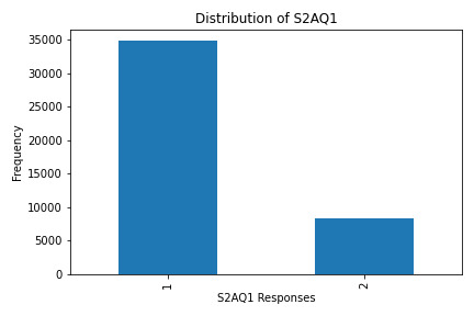
S2AQ1: Ever consumed alcohol?

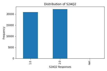
S2AQ2: Consumed at least 12 drinks in the last 12 months?

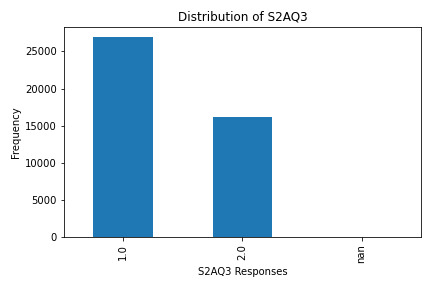
S2AQ3: Frequency of drinking (occasional to regular).

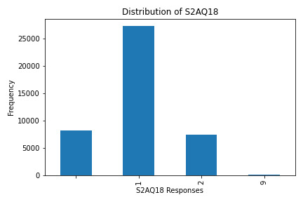
S2AQ18: Frequency of alcohol consumption over time.

This code generates individual (univariate) and paired (bivariate) graphs to analyze the center and spread of each variable and explore relationships between them.

Code and Graphs

Python Code

To recreate this analysis, save this code in a Python file and ensure your CSV dataset is in the same directory. Here’s how to do it:

import pandas as pd import numpy as np import matplotlib.pyplot as plt # Load the dataset data = pd.read_csv('nesarc_pds.csv') # Ensure the CSV file is in the same folder # Selecting variables of interest variables = ['S2AQ1', 'S2AQ2', 'S2AQ3', 'S2AQ18'] # Handling missing data by replacing 9 with NaN data = data.replace(9, np.nan) # Plotting each univariate graph separately # Distribution of S2AQ1 plt.figure(figsize=(6, 4)) data['S2AQ1'].value_counts(dropna=False).sort_index().plot(kind='bar', color='skyblue') plt.title('Distribution of S2AQ1') plt.xlabel('S2AQ1 Responses') plt.ylabel('Frequency') plt.tight_layout() plt.show() # Distribution of S2AQ2 plt.figure(figsize=(6, 4)) data['S2AQ2'].value_counts(dropna=False).sort_index().plot(kind='bar', color='lightcoral') plt.title('Distribution of S2AQ2') plt.xlabel('S2AQ2 Responses') plt.ylabel('Frequency') plt.tight_layout() plt.show() # Distribution of S2AQ3 plt.figure(figsize=(6, 4)) data['S2AQ3'].value_counts(dropna=False).sort_index().plot(kind='bar', color='lightgreen') plt.title('Distribution of S2AQ3') plt.xlabel('S2AQ3 Responses') plt.ylabel('Frequency') plt.tight_layout() plt.show() # Distribution of S2AQ18 plt.figure(figsize=(6, 4)) data['S2AQ18'].value_counts(dropna=False).sort_index().plot(kind='bar', color='plum') plt.title('Distribution of S2AQ18') plt.xlabel('S2AQ18 Responses') plt.ylabel('Frequency') plt.tight_layout() plt.show() # Bivariate analysis between S2AQ1 and S2AQ18 plt.figure(figsize=(8, 6)) pd.crosstab(data['S2AQ1'], data['S2AQ18']).plot(kind='bar', stacked=True, colormap='viridis') plt.title('Association between Alcohol Consumption and Frequency (S2AQ1 vs. S2AQ18)') plt.xlabel('Ever Consumed Alcohol (S2AQ1)') plt.ylabel('Count') plt.tight_layout() plt.show()

What the Graphs Reveal

S2AQ1 (Ever Consumed Alcohol): Most respondents answered "yes," indicating a significant percentage have tried alcohol.

S2AQ2 (12+ Drinks in Last 12 Months): A smaller group responded affirmatively, showing fewer people have consumed 12+ drinks recently.

S2AQ3 (Frequency of Drinking): Responses varied, with data showing a range of drinking frequencies among participants.

S2AQ18 (Frequency of Alcohol Consumption): This variable had the highest counts for lower-frequency responses, indicating occasional consumption.

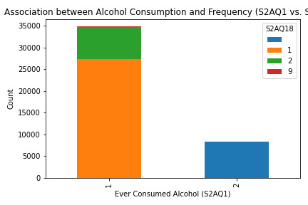
Bivariate Analysis (S2AQ1 and S2AQ18)

The stacked bar chart shows an association between ever consuming alcohol (S2AQ1) and consumption frequency (S2AQ18). While many respondents have consumed alcohol, fewer continue to drink regularly, reflecting a potential drop-off in consistent drinking habits.

Summary: In this assignment, I analyzed alcohol consumption data by examining four survey variables using Python. Through univariate graphs, I visualized the distribution and frequency of responses for each variable, revealing that while many respondents have tried alcohol (S2AQ1), fewer reported frequent consumption. Additionally, the bivariate analysis between initial alcohol consumption (S2AQ1) and recent drinking frequency (S2AQ18) highlighted a drop-off in regular drinking among participants. This exercise demonstrated how data visualization can clarify behavioral trends and provided a practical approach to understanding patterns in alcohol use.

[alcohol-consumption-dependence]

Analyzing Alcohol Consumption: Data Management and Frequency Distributions in Python

Python Program:

import pandas import numpy as np

data = pandas.read_csv('nesarc_pds.csv', low_memory=False)

print(len(data)) # Number of observations (rows) print(len(data.columns)) # Number of variables (columns)

Drank atleast 12 alcoholic drinks in last 12 months

sub1=data["S2AQ2"].value_counts(sort=False)

make a copy of inserted data

sub2 = sub1.copy()

print("counts for original S2AQ2") c1= sub2 print(c1)

sub2 = sub2.replace(9, np.nan)

print('counts for S2AQ2 with 9 set to nan') c2= sub2 print(c2)

Drank atleast 1 alcoholic drinks in last 12 months

sub3=data["S2AQ3"].value_counts(sort=False)

make a copy of inserted data

sub4 = sub3.copy()

print("counts for original S2AQ3") c3= sub3 print(c3)

sub3 = sub3.replace(9, np.nan)

print('counts for S2AQ3 with 9 set to nan') c3= sub3 print(c3)

Family or friends told to cut down on drinking

sub5=data["S2AQ18"].value_counts(sort=False)

make a copy of inserted data

sub5 = sub1.copy()

print("counts for original S2AQ18") c1= sub5 print(c1)

sub6 = sub5.replace(9, np.nan)

print('counts for S2AQ18 with 9 set to nan') c2= sub6 print(c2)

Interpretation of Results

Variable 1: This variable primarily took values in numeric numbers. Most frequent values were 1 indicating a yes answer to the questions, and value of 9 was used to display data that could be labelled as missing which is replaced in this code to "nan" using the NumPy library.

Variable 2: This distribution reflects that most of the survey population had at some point in their life drank alcoholic drinks. Most of the population answered "1" yes to drinking. 1 was seen as the most common answer in the data set.

Variable 3: The distribution showed a clear grouping, with most of the survey population having drank alcoholic drinks at some point in their life. However, an anomaly was noticed in S2AQ2 when more people answered "2" or no when asked if they had consumed atleast 12 alcoholic drinks in last 12 months. Summary: In this post, I explored alcohol consumption data, managing variables in Python to create meaningful insights. By handling missing data, recoding variables, and analyzing frequency distributions, I highlighted key trends. Most respondents had consumed alcohol at some point (indicated by a frequent "yes" answer), and missing data was coded as "nan" to ensure clarity. Interestingly, while many had consumed alcohol, fewer had done so in the past year, as reflected by a higher count of "no" answers to recent drinking. This assignment emphasized how strategic data management can unveil important behavioral patterns and anomalies within survey data.

[alcohol-consumption-dependence]

Analyzing Alcohol Consumption Patterns: A Python Frequency Distribution Approach

Program:

python

Copy code

from tabulate import tabulate data = [['1', 34827, '80.8182', '34827', 80.8182], ['2', 8266, '19.1818', '43093', 100]] print("--------------------------------------------------------------------------------------------") title = "S2AQ1 Drank atleast 1 drink in life" print(title.center(75)) print("--------------------------------------------------------------------------------------------") print(tabulate(data, headers=['Answer', 'Frequency', 'Percentage', 'Cumulative Frequency', 'Cumulative Percentage'], tablefmt='orgtbl')) print("--------------------------------------------------------------------------------------------") data = [['1', 20836, '48.3512', '20836', 48.3512], ['2', 22225, '51.5745', '43061', 99.9257], ['9', 32, '00.0743', '43093', 100]] print("--------------------------------------------------------------------------------------------") title = "S2AQ2 Drank atleast 12 alcoholic drinks in last 12 months" print(title.center(75)) print("--------------------------------------------------------------------------------------------") print(tabulate(data, headers=['Answer', 'Frequency', 'Percentage', 'Cumulative Frequency', 'Cumulative Percentage'], tablefmt='orgtbl')) print("--------------------------------------------------------------------------------------------") data = [['1', 26946, '62.5299', '26946', 62.5299], ['2', 16116, '37.3982', '43062', 99.9281], ['9', 31, '00.0719', '43093', 100]] print("--------------------------------------------------------------------------------------------") title = "S2AQ3 Drank atleast 1 alcoholic drink in last 12 months" print(title.center(75)) print("--------------------------------------------------------------------------------------------") print(tabulate(data, headers=['Answer', 'Frequency', 'Percentage', 'Cumulative Frequency', 'Cumulative Percentage'], tablefmt='orgtbl')) print("--------------------------------------------------------------------------------------------") data = [['1', 27324, '63.407', '27324', 63.407], ['2', 7427, '17.2348', '34751', 80.6418], ['9', 76, '00.1764', '34827', 80.8182], ['BL', 8266, '19.1818', '43093', 100]] print("--------------------------------------------------------------------------------------------") title = "S2AQ18 Family or friends told to cut down on drinking" print(title.center(75)) print("--------------------------------------------------------------------------------------------") print(tabulate(data, headers=['Answer', 'Frequency', 'Percentage', 'Cumulative Frequency', 'Cumulative Percentage'], tablefmt='orgtbl')) print("--------------------------------------------------------------------------------------------")

Output:

Here are the frequency distributions for three variables:

S2AQ1: Drank atleast 1 drink in life

S2AQ2: Drank atleast 12 alcoholic drinks in last 12 months

S2AQ18: Family or friends told to cut down on drinking

Analysis:

The frequency tables provide insights into the behavior and experiences of respondents regarding alcohol consumption. The majority of respondents reported drinking at least once in their life, and a significant portion also consumed alcohol frequently in the past 12 months. The data also shows very minimal missing data (coded as '9'), and these observations help us understand drinking patterns and the social feedback individuals receive.

[alcohol-consumption-dependence]

Exploring the Demographic Predictors of Alcohol Dependence Among U.S. Adults: A Data-Driven Approach

Introduction: Millions of people in the United States are dependent on alcohol, which is a major public health problem. Knowing what causes people to become dependent on booze can help people come up with more effective ways to help them and better support systems. We use data from the NESARC Wave 1 study to look at the demographic factors that can help us identify who will become dependent on alcohol as an adult in the United States. In particular, we look at how things like age, gender, and socioeconomic position are linked to alcohol dependence.

Research Question: What factors, like age, sex, and socioeconomic position, can be used to predict alcohol dependence in adults in the United States?

Methodology:   The information used for this study comes from the NESARC Wave 1 study's Sections 2A (Alcohol Use), 2B (Alcohol Abuse or Dependence), and 2C (Alcohol Treatment Utilization). We focused on a small group of variables that show trends of alcohol use, diagnoses of alcohol dependence, and important demographic information.

Key Variables:

booze Consumption: How often, how much, and how you use booze. Alcohol Dependence: The diagnostic conditions for alcohol dependence were met. Age, gender, income, amount of education, and employment status are all examples of demographic variables.

Hypothesis: Based on earlier research, we think that being younger, male, having less money, and not having as much education are all linked to a higher chance of becoming dependent on alcohol. This idea comes from research that shows people from lower-income groups are more likely to have drug abuse disorders, such as alcohol dependence.

Data Analysis:  Statistical methods like logistic regression will be used to look at the link between socioeconomic factors and the chance of becoming dependent on alcohol. We want to find out how each demographic predictor of alcohol consumption affects the other factors by controlling for them.

Findings and Discussion:  This study's findings will help us understand which societal factors are highly linked to alcohol dependence. These results can help shape public health plans and programs that aim to lower the risk of alcohol consumption in groups that are more likely to become dependent on it.

Conclusion: Understanding the societal factors that lead to alcoholism is important for creating successful programs for prevention and treatment. The goal of using data from the NESARC Wave 1 study is to help researchers learn more about the factors that lead to alcohol dependence. This will help lower the number of alcohol-related disorders in the U.S.

References:

Grant, B. F., et al. (2003). "The Alcohol Use Disorder and Associated Disabilities Interview Schedule (AUDADIS-IV)." NIAAA is the National Institute on Alcohol Abuse and Alcoholism. Hasin, D. S., et al. "Prevalence, correlates, disability, and comorbidity of DSM-IV alcohol abuse and dependence in the United States: results from the National Epidemiologic Survey on Alcohol and Related Conditions." No. 64(7), 830–842, Archives of General Psychiatry. The study by Johnson, P., et al. (2010) is called "Socioeconomic disparities in substance use and related behaviors." 64(5), 406-412, in the Journal of Epidemiology and Community Health.

[alcohol-consumption-dependence]

Data Management and Visualization Course

This will serve as the blog for my Data Management and Visualization course available on Coursera