
I'm a space blogger, who writes for www.facethe.space.
Don't wanna be here? Send us removal request.
Statistics
We looked inside some of the posts by neeltron-blog and here's what we found interesting.
Average Info
Notes Per Post
1
Likes Per Post
1
Reblog Per Post
0
Reply Per Post
0
Time Between Posts
1 month
Number of Posts By Type
Text
4
Link
13
Last Seen Tumblr Blogs


Fun Fact
Tumblr was acquired by Yahoo for $1.1B in 2013.
Text
Machine Learning for Data Analysis - Week 4 Assignment
Program
# -*- coding: utf-8 -*-
"""
Created on Tue Jun 9 06:40:12 2020
@author: Neel
"""
from pandas import pandas, DataFrame
import pandas as pd
import numpy as np
import matplotlib.pylab as plt
from sklearn.model_selection import train_test_split
from sklearn import preprocessing
from sklearn.cluster import KMeans
data = pd.read_csv("Data Management and Visualization/Mars Crater Dataset.csv")
data_clean = data.dropna()
cluster = data_clean[["LATITUDE_CIRCLE_IMAGE", "LONGITUDE_CIRCLE_IMAGE", "DEPTH_RIMFLOOR_TOPOG", "DIAM_CIRCLE_IMAGE"]]
print(cluster.describe())
clustervar = cluster.copy()
clustervar["LATITUDE_CIRCLE_IMAGE"] = preprocessing.scale(clustervar["LATITUDE_CIRCLE_IMAGE"].astype("float64"))
clustervar["LONGITUDE_CIRCLE_IMAGE"] = preprocessing.scale(clustervar["LONGITUDE_CIRCLE_IMAGE"].astype("float64"))
clustervar["DIAM_CIRCLE_IMAGE"] = preprocessing.scale(clustervar["DIAM_CIRCLE_IMAGE"].astype("float64"))
clustervar["DEPTH_RIMFLOOR_TOPOG"] = preprocessing.scale(clustervar["DEPTH_RIMFLOOR_TOPOG"].astype("float64"))
clus_train, clus_test = train_test_split(clustervar, test_size = 0.3, random_state = 123)
from scipy.spatial.distance import cdist
clusters = range(1, 10)
meandist = []
for k in clusters:
model = KMeans(n_clusters = k)
model.fit(clus_train)
clus_assign = model.predict(clus_train)
meandist.append(sum(np.min(cdist(clus_train, model.cluster_centers_, "euclidean"), axis = 1)) / clus_train.shape[0])
plt.plot(clusters, meandist)
plt.xlabel("Number of Clusters")
plt.ylabel("Average distance")
plt.title("Selecting k with the elbow method")
model3 = KMeans(n_clusters = 4)
model3.fit(clus_train)
clusassign = model3.predict(clus_train)
from sklearn.decomposition import PCA
pca_3 = PCA(2)
plot_columns = pca_3.fit_transform(clus_train)
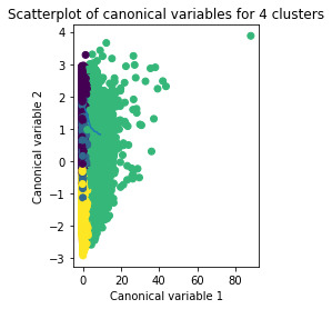
plt.scatter(x = plot_columns[:, 0], y = plot_columns[:, 1], c = model3.labels_,)
plt.xlabel("Canonical variable 1")
plt.ylabel("Canonical variable 2")
plt.title("Scatterplot of canonical variables for 4 clusters")
plt.show()
clus_train.reset_index(level = 0, inplace = True)
cluslist = list(clus_train['index'])
labels = list(model3.labels_)
newlist = dict(zip(cluslist, labels))
print(newlist)
newclus = DataFrame.from_dict(newlist, orient = "index")
print(newclus)
newclus.columns = ["cluster"]
newclus.reset_index(level = 0, inplace = True)
merged_train = pd.merge(clus_train, newclus, on = "index")
print(merged_train.head(n = 100))
merged_train.cluster.value_counts()
clustergrp = merged_train.groupby("cluster").mean()
print("Clustering variable means by cluster")
print(clustergrp)
layer_data = data_clean["NUMBER_LAYERS"]
layer_train, layer_test = train_test_split(layer_data, test_size = 0.3, random_state = 123)
layer_train1 = pd.DataFrame(layer_train)
layer_train1.reset_index(level = 0, inplace = True)
merged_train_all = pd.merge(layer_train1, merged_train, on = "index")
sub1 = merged_train_all[["NUMBER_LAYERS", "cluster"]].dropna()
import statsmodels.formula.api as smf
import statsmodels.stats.multicomp as multi
layermod = smf.ols(formula = "NUMBER_LAYERS ~ C(cluster)", data = sub1).fit()
print(layermod.summary())
print("means for number of layers by cluster")
m1 = sub1.groupby("cluster").mean()
print(m1)
print("standard deviations of number of layers by clusters")
s1 = sub1.groupby("cluster").std()
print(s1)
mc1 = multi.MultiComparison(sub1["NUMBER_LAYERS"], sub1["cluster"])
res1 = mc1.tukeyhsd()
print(res1.summary())
Output
LATITUDE_CIRCLE_IMAGE ... DIAM_CIRCLE_IMAGE
count 384343.000000 ... 384343.000000
mean -7.199209 ... 3.556686
std 33.608966 ... 8.591993
min -86.700000 ... 1.000000
25% -30.935000 ... 1.180000
50% -10.079000 ... 1.530000
75% 17.222500 ... 2.550000
max 85.702000 ... 1164.220000
[8 rows x 4 columns]
15516 0
344967 1
172717 3
378336 1
346725 1
..
192476 0
17730 0
28030 0
277869 1
249342 2
[269040 rows x 1 columns]
index LATITUDE_CIRCLE_IMAGE ... DIAM_CIRCLE_IMAGE cluster
0 15516 1.528797 ... -0.259159 0
1 344967 -0.961762 ... -0.297567 1
2 172717 -0.503015 ... -0.287092 3
3 378336 -1.746048 ... -0.235881 1
4 346725 -1.629978 ... 0.138887 1
.. ... ... ... ... ...
95 153715 -0.058401 ... 0.062071 3
96 330653 -1.456780 ... -0.295239 3
97 57613 1.591102 ... -0.280108 0
98 6871 1.850348 ... 0.162164 0
99 256026 -0.029182 ... -0.232390 1
[100 rows x 6 columns]
Clustering variable means by cluster
index ... DIAM_CIRCLE_IMAGE
cluster ...
0 69195.992176 ... -0.149308
1 265614.659819 ... -0.133282
2 201712.042174 ... 2.557181
3 239120.537881 ... -0.141078
[4 rows x 5 columns]
OLS Regression Results
==============================================================================
Dep. Variable: NUMBER_LAYERS R-squared: 0.120
Model: OLS Adj. R-squared: 0.120
Method: Least Squares F-statistic: 1.217e+04
Date: Tue, 09 Jun 2020 Prob (F-statistic): 0.00
Time: 22:54:30 Log-Likelihood: -45298.
No. Observations: 269040 AIC: 9.060e+04
Df Residuals: 269036 BIC: 9.065e+04
Df Model: 3
Covariance Type: nonrobust
===================================================================================
coef std err t P>|t| [0.025 0.975]
-----------------------------------------------------------------------------------
Intercept 0.0626 0.001 63.631 0.000 0.061 0.065
C(cluster)[T.1] -0.0346 0.001 -25.021 0.000 -0.037 -0.032
C(cluster)[T.2] 0.4445 0.003 171.193 0.000 0.439 0.450
C(cluster)[T.3] -0.0321 0.001 -22.965 0.000 -0.035 -0.029
==============================================================================
Omnibus: 262358.235 Durbin-Watson: 2.008
Prob(Omnibus): 0.000 Jarque-Bera (JB): 12985631.133
Skew: 4.851 Prob(JB): 0.00
Kurtosis: 35.623 Cond. No. 5.47
==============================================================================
Warnings:
[1] Standard Errors assume that the covariance matrix of the errors is correctly specified.
means for number of layers by cluster
NUMBER_LAYERS
cluster
0 0.062638
1 0.028054
2 0.507146
3 0.030526
standard deviations of number of layers by clusters
NUMBER_LAYERS
cluster
0 0.290044
1 0.182880
2 0.803107
3 0.185748
Multiple Comparison of Means - Tukey HSD, FWER=0.05
====================================================
group1 group2 meandiff p-adj lower upper reject
----------------------------------------------------
0 1 -0.0346 0.001 -0.0381 -0.031 True
0 2 0.4445 0.001 0.4378 0.4512 True
0 3 -0.0321 0.001 -0.0357 -0.0285 True
1 2 0.4791 0.001 0.4724 0.4857 True
1 3 0.0025 0.2827 -0.0011 0.006 False
2 3 -0.4766 0.001 -0.4833 -0.4699 True
----------------------------------------------------
Graphs

Results
A k-means cluster analysis was conducted to identify underlying subgroups of craters based on their characteristics that could have an impact on their number of layers. Clustering variables included depth, diameter, latitude and longitude of the craters. All clustering variables were standardized to have a mean of 0 and a standard deviation of 1.
Data were randomly split into a training set that included 70% of the observations (N=11900) and a test set that included 30% of the observations (N=5100). A series of k-means cluster analyses were conducted on the training data specifying k=1-9 clusters, using Euclidean distance. The variance in the clustering variables that was accounted for by the clusters (r-square) was plotted for each of the nine cluster solutions in an elbow curve to provide guidance for choosing the number of clusters to interpret.
The elbow curve was inconclusive, suggesting that the 2, 4, 6 and 8-cluster solutions might be interpreted. The results below are for an interpretation of the 4-cluster solution.
The means on the clustering variables showed that, compared to the other clusters, craters in cluster 1 had moderate levels on the clustering variables. They had a relatively low likelihood of having second highest number of layers. Cluster 2 had the lowest levels of the number of layers. On the other hand, cluster 3 clearly included the most number of layers. Cluster 4 has the second lowest number of layers.
In order to externally validate the clusters, an Analysis of Variance (ANOVA) was conducted to test for significant differences between the clusters on the number of layers. A tukey test was used for post hoc comparisons between the clusters. Results indicated significant differences between the clusters on the number of layers. The tukey post hoc comparisons showed significant differences between clusters on number of layers, with the exception that clusters 1 and 3 were not significantly different from each other.
0 notes
Text
Machine Learning for Data Analysis - Week 3 Assignment
Program
# -*- coding: utf-8 -*-
"""
Created on Wed Jun 3 21:41:33 2020
@author: Neel
"""
import pandas as pd
import numpy as np
import matplotlib.pylab as plt
from sklearn.model_selection import train_test_split
from sklearn.linear_model import LassoLarsCV
data = pd.read_csv("Data Management and Visualization/Mars Crater Dataset.csv")
data_clean = data.dropna()
predictors = data_clean[["LATITUDE_CIRCLE_IMAGE", "LONGITUDE_CIRCLE_IMAGE", "DEPTH_RIMFLOOR_TOPOG", "DIAM_CIRCLE_IMAGE"]]
target = data_clean.NUMBER_LAYERS
from sklearn import preprocessing
predictors["LATITUDE_CIRCLE_IMAGE"] = preprocessing.scale(predictors["LATITUDE_CIRCLE_IMAGE"].astype("float64"))
predictors["LONGITUDE_CIRCLE_IMAGE"] = preprocessing.scale(predictors["LONGITUDE_CIRCLE_IMAGE"].astype("float64"))
predictors["DIAM_CIRCLE_IMAGE"] = preprocessing.scale(predictors["DIAM_CIRCLE_IMAGE"].astype("float64"))
predictors["DEPTH_RIMFLOOR_TOPOG"] = preprocessing.scale(predictors["DEPTH_RIMFLOOR_TOPOG"].astype("float64"))
pred_train, pred_test, tar_train, tar_test = train_test_split(predictors, target, test_size = 0.3, random_state = 123)
model = LassoLarsCV(cv = 10, precompute = False)
res = model.fit(pred_train, tar_train)
print(dict(zip(predictors.columns, model.coef_)))
m_log_alphas = -np.log10(model.alphas_)
ax = plt.gca()
plt.plot(m_log_alphas, model.coef_path_.T)
plt.axvline(-np.log10(model.alpha_), linestyle = "--", color = "k", label = "alpha CV")
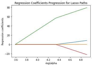
plt.ylabel("Regression coefficients")
plt.xlabel("-log(alpha")
plt.title("Regression Coefficients Progression for Lasso Paths")
# m_log_alphascv = -np.log10(model.cv_alphas_)
# plt.figure()
# plt.plot(m_log_alphascv, model.cv_mse_path_, ":")
# plt.plot(m_log_alphascv, model.cv_mse_path_.mean(axis = -1), "k", label = "Average across the folds", linewidth = 2)
# plt.axvline(-np.log10(model.alpha_), linestyle = "--", color = "k", label = "alpha CV")
# plt.legend()
# plt.ylabel("Mean Squared Error")
# plt.xlabel("-log(alpha")
# plt.title("Mean Squared Error on each fold")
from sklearn.metrics import mean_squared_error
train_error = mean_squared_error(tar_train, model.predict(pred_train))
print("Training Data MSE")
print(train_error)
test_error = mean_squared_error(tar_test, model.predict(pred_test))
print("Test Data MSE")
print(test_error)
rsquared_train = model.score(pred_train, tar_train)
rsquared_test = model.score(pred_test, tar_test)
print("Training Data R Square: ")
print(rsquared_train)
print("Testing Data R Square: ")
print(rsquared_test)
predict = res.predict([[72.76, 164.464, 69, 69]])
print(predict)
Output
C:\Users\Neel\Desktop\Mars-Crater-Research\lasso.py:21: SettingWithCopyWarning:
A value is trying to be set on a copy of a slice from a DataFrame.
Try using .loc[row_indexer,col_indexer] = value instead
See the caveats in the documentation: https://pandas.pydata.org/pandas-docs/stable/user_guide/indexing.html#returning-a-view-versus-a-copy
predictors["LATITUDE_CIRCLE_IMAGE"] = preprocessing.scale(predictors["LATITUDE_CIRCLE_IMAGE"].astype("float64"))
C:\Users\Neel\Desktop\Mars-Crater-Research\lasso.py:22: SettingWithCopyWarning:
A value is trying to be set on a copy of a slice from a DataFrame.
Try using .loc[row_indexer,col_indexer] = value instead
See the caveats in the documentation: https://pandas.pydata.org/pandas-docs/stable/user_guide/indexing.html#returning-a-view-versus-a-copy
predictors["LONGITUDE_CIRCLE_IMAGE"] = preprocessing.scale(predictors["LONGITUDE_CIRCLE_IMAGE"].astype("float64"))
C:\Users\Neel\Desktop\Mars-Crater-Research\lasso.py:23: SettingWithCopyWarning:
A value is trying to be set on a copy of a slice from a DataFrame.
Try using .loc[row_indexer,col_indexer] = value instead
See the caveats in the documentation: https://pandas.pydata.org/pandas-docs/stable/user_guide/indexing.html#returning-a-view-versus-a-copy
predictors["DIAM_CIRCLE_IMAGE"] = preprocessing.scale(predictors["DIAM_CIRCLE_IMAGE"].astype("float64"))
C:\Users\Neel\Desktop\Mars-Crater-Research\lasso.py:24: SettingWithCopyWarning:
A value is trying to be set on a copy of a slice from a DataFrame.
Try using .loc[row_indexer,col_indexer] = value instead
See the caveats in the documentation: https://pandas.pydata.org/pandas-docs/stable/user_guide/indexing.html#returning-a-view-versus-a-copy
predictors["DEPTH_RIMFLOOR_TOPOG"] = preprocessing.scale(predictors["DEPTH_RIMFLOOR_TOPOG"].astype("float64"))
{'LATITUDE_CIRCLE_IMAGE': 0.023351927884135242, 'LONGITUDE_CIRCLE_IMAGE': -0.006999773652777392, 'DEPTH_RIMFLOOR_TOPOG': 0.16868278738287418, 'DIAM_CIRCLE_IMAGE': -0.05816405222722555}
C:\Users\Neel\Desktop\Mars-Crater-Research\lasso.py:33: RuntimeWarning: divide by zero encountered in log10
m_log_alphas = -np.log10(model.alphas_)
C:\Users\Neel\Desktop\Mars-Crater-Research\lasso.py:36: RuntimeWarning: divide by zero encountered in log10
plt.axvline(-np.log10(model.alpha_), linestyle = "--", color = "k", label = "alpha CV")
Training Data MSE
0.07236902854261854
Test Data MSE
0.07287892320974143
Training Data R Square:
0.22286504713654443
Testing Data R Square:
0.21271372919202725
[8.23843645]
Figures now render in the Plots pane by default. To make them also appear inline in the Console, uncheck "Mute Inline Plotting" under the Plots pane options menu.
Graph
Results
A lasso regression analysis was conducted to identify a subset of variables from a pool of 4 categorical and quantitative predictor variables that best predicted a quantitative response variable measuring the number of cohesive layers in craters. Quantitative predictor variables include latitude, longitude, depth and diameter of craters. All predictor variables were standardized to have a mean of zero and a standard deviation of one.
Data were randomly split into a training set that included 70% of the observations (N=11900) and a test set that included 30% of the observations (N=5100). The least angle regression algorithm with k=10 fold cross validation was used to estimate the lasso regression model in the training set, and the model was validated using the test set. The change in the cross validation average (mean) squared error at each step was used to identify the best subset of predictor variables.
Of the 4 predictor variables, all were retained in the selected model. During the estimation process, depth and latitude were most strongly associated with the number of layers.
0 notes
Text
Machine Learning for Data Analysis - Week 2
Program
# -*- coding: utf-8 -*-
"""
Created on Tue May 26 14:10:10 2020
@author: Neel
"""
from pandas import Series, DataFrame
import pandas as pd
import numpy as np
import matplotlib.pylab as plt
from sklearn.model_selection import train_test_split
from sklearn.tree import DecisionTreeClassifier
from sklearn.metrics import classification_report
import sklearn.metrics
from sklearn import datasets
from sklearn.ensemble import ExtraTreesClassifier
from sklearn.ensemble import RandomForestClassifier
import os
os.environ['PATH'] = os.environ['PATH']+';'+os.environ['CONDA_PREFIX']+r"\Library\bin\graphviz"
data = pd.read_csv("Data Management and Visualization/Mars Crater Dataset.csv")
data = data[(data["NUMBER_LAYERS"] >= 0)]
data_clean = data.dropna()
data_clean.dtypes
data_clean.describe()
predictors = data_clean[["LATITUDE_CIRCLE_IMAGE", "LONGITUDE_CIRCLE_IMAGE", "DEPTH_RIMFLOOR_TOPOG", "DIAM_CIRCLE_IMAGE"]]
targets = data_clean.NUMBER_LAYERS
pred_train, pred_test, tar_train, tar_test = train_test_split(predictors, targets, test_size = .4)
print(pred_train.shape)
print(pred_test.shape)
print(tar_train.shape)
print(tar_test.shape)
classifier = RandomForestClassifier(n_estimators = 25)
classifier = classifier.fit(pred_train, tar_train)
predictions = classifier.predict(pred_test)
print(predictions[20])
print(sklearn.metrics.confusion_matrix(tar_test, predictions))
accuracy = sklearn.metrics.accuracy_score(tar_test, predictions)
print(accuracy)
predict = classifier.predict([[72.76, 164.464, 69, 69]])
print(predict)
model = ExtraTreesClassifier()
model.fit(pred_train, tar_train)
print(model.feature_importances_)
trees = range(25)
accuracy = np.zeros(25)
for idx in range(len(trees)):
classifier = RandomForestClassifier(n_estimators = idx + 1)
classifier = classifier.fit(pred_train, tar_train)
predictions = classifier.predict(pred_test)
accuracy[idx] = sklearn.metrics.accuracy_score(tar_test, predictions)
plt.cla()
plt.plot(trees, accuracy)
Output
(230605, 4)
(153738, 4)
(230605,)
(153738,)
0[[144195 1535 130 25 1 0]
[ 3523 2359 238 14 0 0]
[ 593 461 294 26 0 0]
[ 148 57 68 26 2 0]
[ 22 3 11 5 0 1]
[ 1 0 0 0 0 0]]
0.9553526128868595
[0]
[0.21082223 0.19188982 0.33425903 0.26302892]
Efficiency Graph
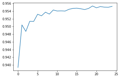
Results
Random forest analysis was performed to evaluate the importance of a series of explanatory variables in predicting a binary, categorical response variable. The following explanatory variables were included as possible contributors to a random forest evaluating the number of layers (my response variable), latitude, longitude, depth of the crater and diameter of the crater.
The explanatory variables with the highest relative importance scores were depths and diameters of the craters. The accuracy of the random forest was 95.5%, with the subsequent growing of multiple trees rather than a single tree, adding little to the overall accuracy of the model, and suggesting that interpretation of random forest is more appropriate.
0 notes
Text
Machine Learning for Data Analysis - Week 1
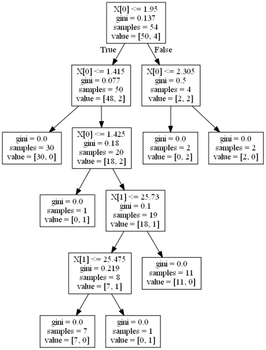
Decision tree analysis was performed to test nonlinear relationships among a series of explanatory variables and a binary, categorical response variable. All possible separations (categorical) or cut points (quantitative) are tested. For the present analyses, the entropy “goodness of split” criterion was used to grow the tree and a cost complexity algorithm was used for pruning the full tree into a final subtree.
The following explanatory variables were included as possible contributors to a classification tree model evaluating the number of layers (my response variable), diameter and depth of the craters.
The depth was the first variable to separate the sample into two subgroups. Craters with depth greater than or equal to 1.95 were more likely to have experimented with depth compared to craters not meeting this cutoff (18.6% vs. 11.2%).
Of the adolescents with deviance scores less than 1.95, a further subdivision was made with the dichotomous variable of depth.
0 notes
Link
0 notes
Link
0 notes
Link
0 notes
Link
0 notes
Link
0 notes
Link
Greetings to all the Space Enthusiasts, have you ever wondered what’s beyond the borders of space-time? Well, if you wanna find out, you’re always welcome to read topics like ‘Time Travel’, ‘Multiverse’, ‘Extraterrestrial Life’, and many more on my blog. Here’s the good news: If you have anything to share with the world, you also have the opportunity to write. Just drop us an email on [email protected]. So, read and share it with your Cosmic friends and family!
1 note
·
View note