#GoogleSQL

[govindhtech]

SQL Pipe Syntax, Now Available In BigQuery And Cloud Logging

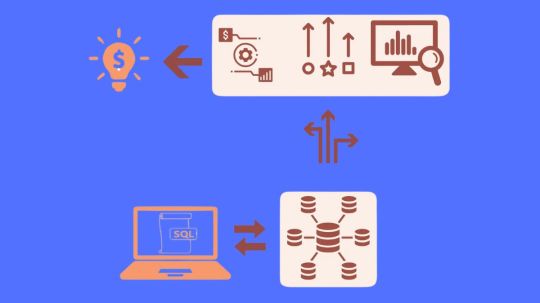
The revolutionary SQL pipe syntax is now accessible in Cloud Logging and BigQuery.

SQL has emerged as the industry standard language for database development. Its well-known syntax and established community have made data access genuinely accessible to everyone. However, SQL isn’t flawless, let’s face it. Several problems with SQL’s syntax make it more difficult to read and write:

Rigid structure: Subqueries or other intricate patterns are needed to accomplish anything else, and a query must adhere to a specific order (SELECT … FROM … WHERE … GROUP BY).

Awkward inside-out data flow: FROM clauses included in subqueries or common table expressions (CTE) are the first step in a query, after which logic is built outward.

Verbose, repetitive syntax: Are you sick of seeing the same columns in every subquery and repeatedly in SELECT, GROUP BY, and ORDER BY?

For novice users, these problems may make SQL more challenging. Reading or writing SQL requires more effort than should be required, even for experienced users. Everyone would benefit from a more practical syntax.

Numerous alternative languages and APIs have been put forth over time, some of which have shown considerable promise in specific applications. Many of these, such as Python DataFrames and Apache Beam, leverage piped data flow, which facilitates the creation of arbitrary queries. Compared to SQL, many users find this syntax to be more understandable and practical.

Presenting SQL pipe syntax

Google Cloud is to simplify and improve the usability of data analysis. It is therefore excited to provide pipe syntax, a ground-breaking invention that enhances SQL in BigQuery and Cloud Logging with the beauty of piped data flow.

Pipe syntax: what is it?

In summary, pipe syntax is an addition to normal SQL syntax that increases the flexibility, conciseness, and simplicity of SQL. Although it permits applying operators in any sequence and in any number of times, it provides the same underlying operators as normal SQL, with the same semantics and essentially the same syntax.

How it operates:

FROM can be used to begin a query.

The |> pipe sign is used to write operators in a consecutive fashion.

Every operator creates an output table after consuming its input table.

Standard SQL syntax is used by the majority of pipe operators:

LIMIT, ORDER BY, JOIN, WHERE, SELECT, and so forth.

It is possible to blend standard and pipe syntax at will, even in the same query.

Impact in the real world at HSBC

After experimenting with a preliminary version in BigQuery and seeing remarkable benefits, the multinational financial behemoth HSBC has already adopted pipe syntax. They observed notable gains in code readability and productivity, particularly when working with sizable JSON collections.

Benefits of integrating SQL pipe syntax

SQL developers benefit from the addition of pipe syntax in several ways. Here are several examples:

Simple to understand

It can be difficult to learn and accept new languages, especially in large organizations where it is preferable for everyone to utilize the same tools and languages. Pipe syntax is a new feature of the already-existing SQL language, not a new language. Because pipe syntax uses many of the same operators and largely uses the same syntax, it is relatively easy for users who are already familiar with SQL to learn.

Learning pipe syntax initially is simpler for users who are new to SQL. They can utilize those operators to express their intended queries directly, avoiding some of the complexities and workarounds needed when writing queries in normal SQL, but they still need to master the operators and some semantics (such as inner and outer joins).

Simple to gradually implement without requiring migrations

As everyone knows, switching to a new language or system may be costly, time-consuming, and prone to mistakes. You don’t need to migrate anything in order to begin using pipe syntax because it is a part of GoogleSQL. All current queries still function, and the new syntax can be used sparingly where it is useful. Existing SQL code is completely compatible with any new SQL. For instance, standard views defined in standard syntax can be called by queries using pipe syntax, and vice versa. Any current SQL does not become outdated or unusable when pipe syntax is used in new SQL code.

No impact on cost or performance

Without any additional layers (such translation proxies), which might increase latency, cost, or reliability issues and make debugging or tweaking more challenging, pipe syntax functions on well-known platforms like BigQuery.

Additionally, there is no extra charge. SQL’s declarative semantics still apply to queries utilizing pipe syntax, therefore the SQL query optimizer will still reorganize the query to run more quickly. Stated otherwise, the performance of queries written in standard or pipe syntax is usually identical.

For what purposes can pipe syntax be used?

Pipe syntax enables you to construct SQL queries that are easier to understand, more effective, and easier to maintain, whether you’re examining data, establishing data pipelines, making dashboards, or examining logs. Additionally, you may use pipe syntax anytime you create queries because it supports the majority of typical SQL operators. A few apps to get you started are as follows:

Debugging queries and ad hoc analysis

When conducting data exploration, you usually begin by examining a table’s rows (beginning with a FROM clause) to determine what is there. After that, you apply filters, aggregations, joins, ordering, and other operations. Because you can begin with a FROM clause and work your way up from there, pipe syntax makes this type of research really simple. You can view the current results at each stage, add a pipe operator, and then rerun the query to view the updated results.

Debugging queries is another benefit of using pipe syntax. It is possible to highlight a query prefix and execute it, displaying the intermediate result up to that point. This is a good feature of queries in pipe syntax: every query prefix up to a pipe symbol is also a legitimate query.

Lifecycle of data engineering

Data processing and transformation become increasingly difficult and time-consuming as data volume increases. Building, modifying, and maintaining a data pipeline typically requires a significant technical effort in contexts with a lot of data. Pipe syntax simplifies data engineering with its more user-friendly syntax and linear query structure. Bid farewell to the CTEs and highly nested queries that tend to appear whenever standard SQL is used. This latest version of GoogleSQL simplifies the process of building and managing data pipelines by reimagining how to parse, extract, and convert data.

Using plain language and LLMs with SQL

For the same reasons that SQL can be difficult for people to read and write, research indicates that it can also be difficult for large language models (LLMs) to comprehend or produce. Pipe syntax, on the other hand, divides inquiries into separate phases that closely match the intended logical data flow. A desired data flow may be expressed more easily by the LLM using pipe syntax, and the generated queries can be made more simpler and easier for humans to understand. This also makes it much easier for humans to validate the created queries.

Because it’s much simpler to comprehend what’s happening and what’s feasible, pipe syntax also enables improved code assistants and auto-completion. Additionally, it allows for suggestions for local modifications to a single pipe operator rather than global edits to an entire query. More natural language-based operators in a query and more intelligent AI-generated code suggestions are excellent ways to increase user productivity.

Discover the potential of pipe syntax right now

Because SQL is so effective, it has been the worldwide language of data for 50 years. When it comes to expressing queries as declarative combinations of relational operators, SQL excels in many things.

However, that does not preclude SQL from being improved. By resolving SQL’s primary usability issues and opening up new possibilities for interacting with and expanding SQL, pipe syntax propels SQL into the future. This has nothing to do with creating a new language or replacing SQL. Although SQL with pipe syntax is still SQL, it is a better version of the language that is more expressive, versatile, and easy to use.

Read more on Govindhtech.com

[tottaz]

Excel with Google Cloud SQL Server

#Excel with #Google #Cloud #SQL #Server #microsoft #google #googlesql

Google has added the SQL server as an option to the Google Cloud SQL service. In this article, I will explore how to set up a Google Cloud SQL server I received a question what was the best way to move a Cloud BI server to the GCP Cloud, and run VB Script from an Excel against that server.

(more…)

[govindhtech]

An Introduction Of Pipe Syntax In BigQuery And Cloud Logging

Organizations looking to improve user experiences, boost security, optimize performance, and comprehend application behavior now find that log data is a priceless resource. However, the sheer amount and intricacy of logs produced by contemporary applications can be debilitating.

Google Cloud is to give you the most effective and user-friendly solutions possible so you can fully utilize your log data. Google Cloud is excited to share with us a number of BigQuery and Cloud Logging advancements that will completely transform how you handle, examine, and use your log data.

Pipe syntax

An improvement to GoogleSQL called pipe syntax allows for a linear query structure that makes writing, reading, and maintaining your queries simpler.

Pipe syntax is supported everywhere in GoogleSQL writing. The operations supported by pipe syntax are the same as those supported by conventional GoogleSQL syntax, or standard syntax, such as joining, filtering, aggregating and grouping, and selection. However, the operations can be applied in any sequence and many times. Because of the linear form of pipe syntax, you may write queries so that the logical steps taken to construct the result table are reflected in the order in which the query syntax is written.

Pipe syntax queries are priced, run, and optimized in the same manner as their standard syntax equivalents. To minimize expenses and maximize query computation, adhere to the recommendations when composing queries using pipe syntax.

There are problems with standard syntax that can make it challenging to comprehend, write, and maintain. The way pipe syntax resolves these problems is illustrated in the following table:

SQL for log data reimagined with BigQuery pipe syntax

The days of understanding intricate, layered SQL queries are over. A new era of SQL is introduced by BigQuery pipe syntax, which was created with the semi-structured nature of log data in mind. The top-down, intuitive syntax of BigQuery’s pipe syntax is modeled around the way you typically handle data manipulations. According to Google’s latest research, this method significantly improves the readability and writability of queries. The pipe sign (|>) makes it very simple to visually distinguish between distinct phases of a query, which makes understanding the logical flow of data transformation much easier. Because each phase is distinct, self-contained, and unambiguous, your questions become easier to understand for both you and your team.

The pipe syntax in BigQuery allows you to work with your data in a more efficient and natural way, rather than merely writing cleaner SQL. Experience quicker insights, better teamwork, and more time spent extracting value rather than wrangling with code.

This simplified method is very effective in the field of log analysis.

The key to log analysis is investigation. Rarely is log analysis a simple question-answer process. Finding certain events or patterns in mountains of data is a common task when analyzing logs. Along the way, you delve deeper, learn new things, and hone your strategy. This iterative process is embraced by pipe syntax. To extract those golden insights, you can easily chain together filters (WHERE), aggregations (COUNT), and sorting (ORDER BY). Additionally, you can simply modify your analysis on the fly by adding or removing phases as you gain new insights from your data processing.

Let’s say you wish to determine how many users in January were impacted by the same faults more than 100 times in total. The data flows through each transformation as demonstrated by the pipe syntax’s linear structure, which starts with the table, filters by dates, counts by user ID and error type, filters for errors more than 100, and then counts the number of users impacted by the same faults.

— Pipe Syntax FROM log_table |> WHERE datetime BETWEEN DATETIME ‘2024-01-01’ AND ‘2024-01-31’ |> AGGREGATE COUNT(log_id) AS error_count GROUP BY user_id, error_type |> WHERE error_count>100 |> AGGREGATE COUNT(user_id) AS user_count GROUP BY

A subquery and non-linear structure are usually needed for the same example in standard syntax.

Currently, BigQuery pipe syntax is accessible in private preview. Please use this form to sign up for a private preview and watch this introductory video.

Beyond syntax: adaptability and performance

BigQuery can now handle JSON with more power and better performance, which will speed up your log analytics operations even more. Since most logs contain json data, it anticipate that most customers will find log analytics easier to understand as a result of these modifications.

Enhanced Point Lookups: Significantly speed up queries that filter on timestamps and unique IDs by use BigQuery’s numeric search indexes to swiftly identify important events in large datasets.

Robust JSON Analysis: With BigQuery’s JSON_KEYS function and JSONPath traversal capability, you can easily parse and analyze your JSON-formatted log data. Without breaking a sweat, extract particular fields, filter on nested data, and navigate intricate JSON structures.

JSON_KEYS facilitates schema exploration and discoverability by removing distinct JSON keys from JSON data.Query Results JSON_KEYS(JSON '{"a":{"b":1}}')["a", "a.b"]JSON_KEYS(JSON '{"a":[{"b":1}, {"c":2}]}', mode => "lax")["a", "a.b", "a.c"]JSON_KEYS(JSON '[[{"a":1},{"b":2}]]', mode => "lax recursive")["a", "b"]

You don’t need to use verbose UNNEST to download JSON arrays when using JSONPath with LAX modes. How to retrieve every phone number from the person field, both before and after, is demonstrated in the example below:

Log Analytics for Cloud Logging: Completing the Picture

Built on top of BigQuery, Log Analytics in Cloud Logging offers a user interface specifically designed for log analysis. By utilizing the JSON capabilities for charting, dashboarding, and an integrated date/time picker, Log Analytics is able to enable complex queries and expedite log analysis. It is also adding pipe syntax to Log Analytics (in Cloud Logging) to make it easier to include these potent features into your log management process. With the full potential of BigQuery pipe syntax, improved lookups, and JSON handling, you can now analyze your logs in Log Analytics on a single, unified platform.

The preview version of Log Analytics (Cloud Logging) now allows the use of pipe syntax.

Unlock log analytics’ future now

The combination of BigQuery and Cloud Logging offers an unparalleled method for organizing, examining, and deriving useful conclusions from your log data. Discover the power of these new skills by exploring them now.

Using pipe syntax for intuitive querying: an introductory video and documentation

Cloud logging’s Log Analytics provides unified log management and analysis.

Lightning-quick lookups using numeric search indexes – Support

JSON_KEYS and JSON_PATH allow for seamless JSON analysis

Read more on Govindhtech.com

[govindhtech]

BigQuery And Spanner With External Datasets Boosts Insights

BigQuery and Spanner work better together by extending operational insights with external datasets.

Analyzing data from several databases has always been difficult for data analysts. They must employ ETL procedures to transfer data from transactional databases into analytical data storage due to data silos. If you have data in both Spanner and BigQuery, BigQuery has made the issue somewhat simpler to tackle.

You might use federated queries to wrap your Spanner query and integrate the results set with BigQuery using a TVF by using the EXTERNAL_QUERY table-valued function (TVF). Although effective, this method had drawbacks, including restricted query monitoring and query optimization insights, and added complexity by having the analyst to create intricate SQL when integrating data from two sources.

Google Cloud to provides today public preview of BigQuery external datasets for Spanner, which represents a significant advancement. Data analysts can browse, analyze, and query Spanner tables just as they would native BigQuery tables with to this productivity-boosting innovation that connects Spanner schema to BigQuery datasets. BigQuery and Spanner tables may be used with well-known GoogleSQL to create analytics pipelines and dashboards without the need for additional data migration or complicated ETL procedures.

Using Spanner external datasets to get operational insights

Gathering operational insights that were previously impossible without transferring data is made simple by spanner external databases.

Operational dashboards: A service provider uses BigQuery for historical analytics and Spanner for real-time transaction data. This enables them to develop thorough real-time dashboards that assist frontline employees in carrying out daily service duties while providing them with direct access to the vital business indicators that gauge the effectiveness of the company.

Customer 360: By combining extensive analytical insights on customer loyalty from purchase history in their data lake with in-store transaction data, a retail company gives contact center employees a comprehensive picture of its top consumers.

Threat intelligence: Information security businesses’ Security Operations (SecOps) personnel must use AI models based on long-term data stored in their analytical data store to assess real-time streaming data entering their operations data store. To compare incoming threats with pre-established threat patterns, SecOps staff must be able to query historical and real-time data using familiar SQL via a single interface.

Leading commerce data SaaS firm Attain was among the first to integrate BigQuery external datasets and claims that it has increased data analysts’ productivity.

Advantages of Spanner external datasets

The following advantages are offered by Spanner and BigQuery working together for data analysts seeking operational insights on their transactions and analytical data:

Simplified query writing: Eliminate the need for laborious federated queries by working directly with data in Spanner as if it were already in BigQuery.

Unified transaction analytics: Combine data from BigQuery and Spanner to create integrated dashboards and reports.

Real-time insights: BigQuery continuously asks Spanner for the most recent data, giving reliable, current insights without affecting production Spanner workloads or requiring intricate synchronization procedures.

Low-latency performance: BigQuery speeds up queries against Spanner by using parallelism and Spanner Data Boost features, which produces results more quickly.

How it operates

Suppose you want to include new e-commerce transactions from a Spanner database into your BigQuery searches.

All of your previous transactions are stored in BigQuery, and your analytical dashboards are constructed using this data. But sometimes, you may need to examine the combined view of recent and previous transactions. At that point, you may use BigQuery to generate an external datasets that replicates your Spanner database.

Assume that you have a project called “myproject” in Spanner, along with an instance called “myinstance” and a database called “ecommerce,” where you keep track of the transactions that are currently occurring on your e-commerce website. With the inclusion of the “Link to an external database” option, you may Create an external datasets in BigQuery exactly like any other dataset:Image Credit To Google Cloud

Browse a Spanner external dataset

A chosen Spanner database may also be seen as an external datasets via the Google Cloud console’s BigQuery Studio. You may see all of your Spanner tables by selecting this dataset and expanding it:Image Credit To Google Cloud

Sample queries

You can now run any query you choose on the tables in your external datasets actually, your Spanner database.

Let’s look at today’s transactions using customer segments that BigQuery calculates and stores, for instance:

SELECT o.id, o.customer_id, o.total_value, s.segment_name FROM current_transactions.ecommerce_order o left join crm_dataset.customer_segments s on o.customer_id=s.customer_id WHERE o.order_date = ‘2024-09-01’

Observe that current_transactions is an external datasets that refers to a Spanner database, whereas crm_dataset is a standard BigQuery dataset.

An additional example would be a single view of every transaction a client has ever made, both past and present:

SELECT id, customer_id, total_value FROM current_transactions.ecommerce_order o union transactions_history th

Once again, transactions_history is stored in BigQuery, but current_transactions is an external datasets.

Note that you don’t need to manually transfer the data using any ETL procedures since it is retrieved live from Spanner!

You may see the query plan when the query is finished. You can see how the ecommerce_order table was utilized in a query and how many entries were read from a particular database by selecting the EXECUTION GRAPH tab.

Reda more on Govindhtech.com

[govindhtech]

BigLake Tables: Future of Unified Data Storage And Analytics

Introduction BigLake external tables

This article introduces BigLake and assumes database tables and IAM knowledge. To query data in supported data storage, build BigLake tables and query them using GoogleSQL:

Create Cloud Storage BigLake tables and query.

Create BigLake tables in Amazon S3 and query.

Create Azure Blob Storage BigLake tables and query.

BigLake tables provide structured data queries in external data storage with delegation. Access delegation separates BigLake table and data storage access. Data store connections are made via service account external connections. Users only need access to the BigLake table since the service account retrieves data from the data store. This allows fine-grained table-level row- and column-level security. Dynamic data masking works for Cloud Storage-based BigLake tables. BigQuery Omni explains multi-cloud analytic methods integrating BigLake tables with Amazon S3 or Blob Storage data.

Support for temporary tables

BigLake Cloud Storage tables might be temporary or permanent.

Amazon S3/Blob Storage BigLake tables must last.

Source files multiple

Multiple external data sources with the same schema may be used to generate a BigLake table.

Cross-cloud connects

Query across Google Cloud and BigQuery Omni using cross-cloud joins. Google SQL JOIN can examine data from AWS, Azure, public datasets, and other Google Cloud services. Cross-cloud joins prevent data copying before queries.

BigLake table may be used in SELECT statements like any other BigQuery table, including in DML and DDL operations that employ subqueries to obtain data. BigQuery and BigLake tables from various clouds may be used in the same query. BigQuery tables must share a region.

Cross-cloud join needs permissions

Ask your administrator to give you the BigQuery Data Editor (roles/bigquery.dataEditor) IAM role on the project where the cross-cloud connect is done. See Manage project, folder, and organization access for role granting.

Cross-cloud connect fees

BigQuery splits cross-cloud join queries into local and remote portions. BigQuery treats the local component as a regular query. The remote portion constructs a temporary BigQuery table by performing a CREATE TABLE AS SELECT (CTAS) action on the BigLake table in the BigQuery Omni region. This temporary table is used for your cross-cloud join by BigQuery, which deletes it after eight hours.

Data transmission expenses apply to BigLake tables. BigQuery reduces these expenses by only sending the BigLake table columns and rows referenced in the query. Google Cloud propose a thin column filter to save transfer expenses. In your work history, the CTAS task shows the quantity of bytes sent. Successful transfers cost even if the primary query fails.

One transfer is from an employees table (with a level filter) and one from an active workers table. BigQuery performs the join after the transfer. The successful transfer incurs data transfer costs even if the other fails.

Limits on cross-cloud join

The BigQuery free tier and sandbox don’t enable cross-cloud joins.

A query using JOIN statements may not push aggregates to BigQuery Omni regions.

Even if the identical cross-cloud query is repeated, each temporary table is utilized once.

Transfers cannot exceed 60 GB. Filtering a BigLake table and loading the result must be under 60 GB. You may request a greater quota. No restriction on scanned bytes.

Cross-cloud join queries have an internal rate limit. If query rates surpass the quota, you may get an All our servers are busy processing data sent between regions error. Retrying the query usually works. Request an internal quota increase from support to handle more inquiries.

Cross-cloud joins are only supported in colocated BigQuery regions, BigQuery Omni regions, and US and EU multi-regions. Cross-cloud connects in US or EU multi-regions can only access BigQuery Omni data.

Cross-cloud join queries with 10+ BigQuery Omni datasets may encounter the error “Dataset was not found in location “. When doing a cross-cloud join with more than 10 datasets, provide a location to prevent this problem. If you specifically select a BigQuery region and your query only includes BigLake tables, it runs as a cross-cloud query and incurs data transfer fees.

Can’t query _FILE_NAME pseudo-column with cross-cloud joins.

WHERE clauses cannot utilize INTERVAL or RANGE literals for BigLake table columns.

Cross-cloud join operations don’t disclose bytes processed and transmitted from other clouds. Child CTAS tasks produced during cross-cloud query execution have this information.

Only BigQuery Omni regions support permitted views and procedures referencing BigQuery Omni tables or views.

No pushdowns are performed to remote subqueries in cross-cloud queries that use STRUCT or JSON columns. Create a BigQuery Omni view that filters STRUCT and JSON columns and provides just the essential information as columns to enhance speed.

Inter-cloud joins don’t allow time travel queries.

Connectors

BigQuery connections let you access Cloud Storage-based BigLake tables from other data processing tools. BigLake tables may be accessed using Apache Spark, Hive, TensorFlow, Trino, or Presto. The BigQuery Storage API enforces row- and column-level governance on all BigLake table data access, including connectors.

In the diagram below, the BigQuery Storage API allows Apache Spark users to access approved data:Image Credit To Google Cloud

The BigLake tables on object storage

BigLake allows data lake managers to specify user access limits on tables rather than files, giving them better control.

Google Cloud propose utilizing BigLake tables to construct and manage links to external object stores because they simplify access control.

External tables may be used for ad hoc data discovery and modification without governance.

Limitations

BigLake tables have all external table constraints.

BigQuery and BigLake tables on object storage have the same constraints.

BigLake does not allow Dataproc Personal Cluster Authentication downscoped credentials. For Personal Cluster Authentication, utilize an empty Credential Access Boundary with the “echo -n “{}” option to inject credentials.

Example: This command begins a credential propagation session in myproject for mycluster:

gcloud dataproc clusters enable-personal-auth-session \ --region=us \ --project=myproject \ --access-boundary=<(echo -n "{}") \ mycluster

The BigLake tables are read-only. BigLake tables cannot be modified using DML or other ways.

These formats are supported by BigLake tables:

Avro

CSV

Delta Lake

Iceberg

JSON

ORC

Parquet

BigQuery requires Apache Iceberg’s manifest file information, hence BigLake external tables for Apache Iceberg can’t use cached metadata.

AWS and Azure don’t have BigQuery Storage API.

The following limits apply to cached metadata:

Only BigLake tables that utilize Avro, ORC, Parquet, JSON, and CSV may use cached metadata.

Amazon S3 queries do not provide new data until the metadata cache refreshes after creating, updating, or deleting files. This may provide surprising outcomes. After deleting and writing a file, your query results may exclude both the old and new files depending on when cached information was last updated.

BigLake tables containing Amazon S3 or Blob Storage data cannot use CMEK with cached metadata.

Secure model

Managing and utilizing BigLake tables often involves several organizational roles:

Managers of data lakes. Typically, these administrators administer Cloud Storage bucket and object IAM policies.

Data warehouse managers. Administrators usually edit, remove, and create tables.

A data analyst. Usually, analysts read and query data.

Administrators of data lakes create and share links with data warehouse administrators. Data warehouse administrators construct tables, configure restricted access, and share them with analysts.

Performance metadata caching

Cacheable information improves BigLake table query efficiency. Metadata caching helps when dealing with several files or hive partitioned data. BigLake tables that cache metadata include:

Amazon S3 BigLake tables

BigLake cloud storage

Row numbers, file names, and partitioning information are included. You may activate or disable table metadata caching. Metadata caching works well for Hive partition filters and huge file queries.

Without metadata caching, table queries must access the external data source for object information. Listing millions of files from the external data source might take minutes, increasing query latency. Metadata caching lets queries split and trim files faster without listing external data source files.

Two properties govern this feature:

Cache information is used when maximum staleness is reached.

Metadata cache mode controls metadata collection.

You set the maximum metadata staleness for table operations when metadata caching is enabled. If the interval is 1 hour, actions against the table utilize cached information if it was updated within an hour. If cached metadata is older than that, Amazon S3 or Cloud Storage metadata is retrieved instead. Staleness intervals range from 30 minutes to 7 days.

Cache refresh may be done manually or automatically:

Automatic cache refreshes occur at a system-defined period, generally 30–60 minutes. If datastore files are added, destroyed, or updated randomly, automatically refreshing the cache is a good idea. Manual refresh lets you customize refresh time, such as at the conclusion of an extract-transform-load process.

Use BQ.REFRESH_EXTERNAL_METADATA_CACHE to manually refresh the metadata cache on a timetable that matches your needs. You may selectively update BigLake table information using subdirectories of the table data directory. You may prevent superfluous metadata processing. If datastore files are added, destroyed, or updated at predetermined intervals, such as pipeline output, manually refreshing the cache is a good idea.

Dual manual refreshes will only work once.

The metadata cache expires after 7 days without refreshment.

Manual and automated cache refreshes prioritize INTERACTIVE queries.

To utilize automatic refreshes, establish a reservation and an assignment with a BACKGROUND job type for the project that executes metadata cache refresh tasks. This avoids refresh operations from competing with user requests for resources and failing if there aren’t enough.

Before setting staleness interval and metadata caching mode, examine their interaction. Consider these instances:

To utilize cached metadata in table operations, you must call BQ.REFRESH_EXTERNAL_METADATA_CACHE every 2 days or less if you manually refresh the metadata cache and set the staleness interval to 2 days.

If you automatically refresh the metadata cache for a table and set the staleness interval to 30 minutes, some operations against the table may read from the datastore if the refresh takes longer than 30 to 60 minutes.

Tables with materialized views and cache

When querying structured data in Cloud Storage or Amazon S3, materialized views over BigLake metadata cache-enabled tables increase speed and efficiency. Automatic refresh and adaptive tweaking are available with these materialized views over BigQuery-managed storage tables.

Integrations

BigLake tables are available via other BigQuery features and gcloud CLI services, including the following.

Hub for Analytics

Analytics Hub supports BigLake tables. BigLake table datasets may be listed on Analytics Hub. These postings provide Analytics Hub customers a read-only linked dataset for their project. Subscribers may query all connected dataset tables, including BigLake.

BigQuery ML

BigQuery ML trains and runs models on BigLake in Cloud Storage.

Safeguard sensitive data

BigLake Sensitive Data Protection classifies sensitive data from your tables. Sensitive Data Protection de-identification transformations may conceal, remove, or obscure sensitive data.

Read more on Govindhtech.com

[govindhtech]

BigQuery Tables For Apache Iceberg Optimize Open Lakehouse

BigQuery tables

Optimized storage for the open lakehouse using BigQuery tables for Apache Iceberg. BigQuery native tables have been supporting enterprise-level data management features including streaming ingestion, ACID transactions, and automated storage optimizations for a number of years. Open-source file formats like Apache Parquet and table formats like Apache Iceberg are used by many BigQuery clients to store data in data lakes.

Google Cloud introduced BigLake tables in 2022 so that users may take advantage of BigQuery’s security and speed while keeping a single copy of their data. BigQuery clients must manually arrange data maintenance and conduct data changes using external query engines since BigLake tables are presently read-only. The “small files problem” during ingestion presents another difficulty. Table writes must be micro-batched due to cloud object storage’ inability to enable appends, necessitating trade-offs between data integrity and efficiency.

Google Cloud provides the first look at BigQuery tables for Apache Iceberg, a fully managed storage engine from BigQuery that works with Apache Iceberg and offers capabilities like clustering, high-throughput streaming ingestion, and autonomous storage optimizations. It provide the same feature set and user experience as BigQuery native tables, but they store data in customer-owned cloud storage buckets using the Apache Iceberg format. Google’s are bringing ten years of BigQuery developments to the lakehouse using BigQuery tables for Apache Iceberg.Image Credit To Google Cloud

BigQuery’s Write API allows for high-throughput streaming ingestion from open-source engines like Apache Spark, and BigQuery tables for Apache Iceberg may be written from BigQuery using the GoogleSQL data manipulation language (DML). This is an example of how to use clustering to build a table:

CREATE TABLE mydataset.taxi_trips CLUSTER BY vendor_id, pickup_datetime WITH CONNECTION us.myconnection OPTIONS ( storage_uri=’gs://mybucket/taxi_trips’, table_format=’ICEBERG’, file_format=’PARQUET’ ) AS SELECT * FROM bigquery-public-data.new_york_taxi_trips.tlc_green_trips_2020;

Fully managed enterprise storage for the lakehouse

Drawbacks of BigQuery tables for Apache Iceberg

The drawbacks of open-source table formats are addressed by BigQuery tables for Apache Iceberg. BigQuery handles table-maintenance duties automatically without requiring client labor when using BigQuery tables for Apache Iceberg. BigQuery automatically re-clusters data, collects junk from files, and combines smaller files into appropriate file sizes to keep the table optimized.

For example, the size of the table is used to adaptively decide the ideal file sizes. BigQuery tables for Apache Iceberg take use of more than ten years of experience in successfully and economically managing automatic storage optimization for BigQuery native tables. OPTIMIZE and VACUUM do not need human execution.

BigQuery tables for Apache Iceberg use Vortex, an exabyte-scale structured storage system that drives the BigQuery storage write API, to provide high-throughput streaming ingestion. Recently ingested tuples are persistently stored in a row-oriented manner in BigQuery tables for Apache Iceberg, which regularly convert them to Parquet. The open-source Spark and Flink BigQuery connections provide parallel readings and high-throughput ingestion. You may avoid maintaining custom infrastructure by using Pub/Sub and Datastream to feed data into BigQuery tables for Apache Iceberg.

Advantages of using BigQuery tables for Apache Iceberg

Table metadata is stored in BigQuery’s scalable metadata management system for Apache Iceberg tables. BigQuery handles metadata via distributed query processing and data management strategies, and it saves fine-grained information. since of this, BigQuery tables for Apache Iceberg may have a greater rate of modifications than table formats since they are not limited by the need to commit the information to object storage. The table information is tamper-proof and has a trustworthy audit history since authors are unable to directly alter the transaction log.

While expanding support for governance policy management, data quality, and end-to-end lineage via Dataplex, BigQuery tables for Apache Iceberg still support the fine-grained security rules imposed by the storage APIs.Image Credit To Google Cloud

BigQuery tables for Apache Iceberg are used to export metadata into cloud storage Iceberg snapshots. BigQuery metastore, a serverless runtime metadata service that was revealed earlier this year, will shortly register the link to the most recent exported information. Any engine that can comprehend Iceberg may query the data straight from Cloud Storage with to Iceberg metadata outputs.

Find out more

Clients such as HCA Healthcare, one of the biggest healthcare organizations globally, recognize the benefits of using BigQuery tables for Apache Iceberg as their BigQuery storage layer that is compatible with Apache Iceberg, opening up new lakehouse use-cases. All Google Cloud regions now provide a preview of the BigQuery tables for Apache Iceberg.

Can other tools query data stored in BigQuery tables for Apache Iceberg?

Yes, metadata is exported from Apache Iceberg BigQuery tables into cloud storage Iceberg snapshots. This promotes interoperability within the open data ecosystem by enabling any engine that can comprehend the Iceberg format to query the data straight from Cloud Storage.

How secure are BigQuery tables for Apache Iceberg?

The strong security features of BigQuery, including as fine-grained security controls enforced by storage APIs, are carried over into BigQuery tables for Apache Iceberg. Additionally, end-to-end lineage tracking, data quality control, and extra governance policy management layers are made possible via interaction with Dataplex.

Read more on Govindhtech.com