#How to Calculate Standard Deviation in Discrete Series | Explore Tumblr Posts and Blogs

endivesoftware · 4 years

Link

1. Introduction

Introduction: Why Economics?, Meaning and Definitions of Economics, Economic and Non-economic Activities, Economic Groups, Introduction: Statistics, Meaning and Definition of Statistics, Importance of Statistics in Economics, Limitation of Statistics, Key Points, Question Bank, Very Short Answer Type Questions, Short Answer Type Questions, Long Answer Type Questions, Higher Order Thinking Skills [HOTS], Value Based Questions, Multiple Choice Questions (MCQs).

2. Collection of Data

Introduction, Meaning of Collection of Data, Types of Data (Sources of Data), Methods of Collecting Primary Data, Questionnaire and Schedule, Census and Sample Investigation Techniques, Sampling and Non-Sampling Errors, Sources of Secondary Data, Census of India And NSSO, Key Points, Question Bank, Very Short Answer Type Questions, Short Answer Type Questions, Long Answer Type Questions, Higher Order Thinking Skills (HOTS), Value Based Questions, Multiple Choice Questions (MCQs).

3. Organisation of Data

Introduction, Meaning and Definition of Classification, Objectives of Classification, Methods of Classification, Variable, Statistical Series, Individual Series, Discrete Series (Ungrouped Frequency Distribution or Frequency Array), Continuous Series or Grouped Frequency Distribution, Types of Continuous Series, Bivariate Frequency distribution, General Rules for Constructing a Frequency Distribution, or How to prepare a frequency distribution?, Key Points, Question Bank, Very Short Answer Type Questions, Short Answer Type Questions, Long Answer Type Questions, Numerical Questions, Higher Order Thinking Skills (HOTs), Value Base Questions, Multiple Choice Questions (MCQs).

4. Presentation of Data : Tabular Presentation

Introduction, Textual Presentation of Data (Descriptive Presentation), Tabular Presentation of Data, Objectives of Tabulation, Essential Parts of Table, Type of Table, Solved Examples, Key Points, Question Bank, Very Short Answer Type Questions, Short Answer Type Questions, Long Answer Type Questions, Numerical Questions, Higher Order Thinking Skills (HOTS), Value Based Questions, Multiple Choice Questions (MCQs).

5. Presentation of Data : Diagrammatic Presentation

Introduction, Utility or Advantages of Diagrammatic Presentation, Limitations of Diagrams, General Principles/Rules for Diagrammatic Presentation, Types of Diagrams, Bar Diagram, Pie Diagram, Key Points, Question Bank, Very Short Answer Type Questions, Short Answer Type Question, Long Answer Type Question, Numerical Questions, Higher Order Thinking Skills (HOTS), Multiple Choice Questions (MCQs).

6. Presentation of Data: Graphic Presentation

Introduction, Advantages of Graphic Presentation, Construction of a Graph, False Base Line (Kinked Line), Types of Graphs, Limitation of Graphic Presentations, Key Points, Question Bank, Very Short Answer Type Questions, Short Answer Type Questions, Long Answer Type Questions, Numerical Questions, Higher Order Thinking Skills (HOTS), Multiple Choice Question (MCQs).

7. Measures of Central Tendency Arithmetic Mean

Introduction, Meaning and Definition, Objectives and Significance or uses of Average, Requisites or Essentials of an Ideal Average, Types or Kinds of Statistical Averages, Arithmetic Mean (X), Calculation of Arithmetic Mean in Different Frequency Distribution (Additional Cases), Calculation of Missing Value, Corrected Mean, Combined Arithmetic Mean, Mathematical Properties of Arithmetic Mean, Merits and Demerits of Arithmetic Mean, Weighted Arithmetic Mean, List of Formulae, Key Points, Question Bank, Very Short Answer Type Questions, Short Answer Type Questions, Long Answer Type Questions, Numerical Questions, Miscellaneous Questions, Multiples Choice Questions (MCQs).

8. Measures of Central Tendency Median and Mode

Median, Determination of Median, Calculation of Median in Different Frequency Distribution (Additional Cases), Partition Values (Measures of Position or Positional Values based on The principle of Median), Mode (Z), Computation of Mode, Calculation of Mode in Different Frequency Distribution (Additional Cases), Relationship between Mean, Median and Mode, Comparison between Mean, Median and Mode, Choice of a Suitable Average, Typical Illustration, List of Formulae, Key Points, Question Bank, Very Short Answer Type Questions, Short Answer Type Questions, Long Answer Type Questions, Numerical Questions, Miscellaneous Questions, Higher Order Thinking Skills (HOTS), Value Based Questions, Multiple Choice Questions (MCQs).

9. Measure of Dispersion

Introduction, Meaning and Definition, Objectives and Significance, Characteristics of Good Measure of Dispersion, Methods of Measurement of Dispersion, Types of Dispersion, Range, Inter-Quartile Range and Quaritle Deviation, Mean Deviation (Average Deviation), Standard Deviation (s), Relationship between Different Measures of Dispersion, Lorenz Curve, Choice of A Suitable Measure of Dispersion, Typical Illustrations, List of Formulae, Key Points, Question Bank, Very Short Answer Type Questions, Short Answer Type Questions, Long Answer Type Questions, Numerical Questions, Higher Order Thinking Skills (HOTS), Multiple Choice Questions (MCQs).

10. Correlation

Introduction, Meaning and Definitions, Types of Correlation, Coefficient of Correlation (r), Degree of Correlation, Techniques or Methods for Measuring Correlation, Scatter Diagram (Dotogram Method), Karl Pearson’s Coefficient of Correlation, Spearman’s Rank Correlation, Typical Illustrations, List of Formulae, Key Points, Question Bank, Very Short Answer Type Questions, Short Answer Type Questions, Long Answer Type Questions, Numerical Questions, Miscellaneous Questions, Higher Order Thinking Skills (HOTS), Value Based Questions, Multiple Choice Questions.

11. Index Numbers

Introduction, Characteristics or Features, Precautions in Constructions of Index Numbers (Problems), Types or Kinds of Index Numbers, Methods of Constructing Price Index Numbers, Simple Index Number (Unweighted), Weighted Index Numbers, Some Important Index Numbers, Significance or Uses of Index Numbers, Limitations of Index Numbers, List of Formulae, Key Points, Question Bank, Very Short Answer Type Questions, Short Answer Type Questions, Long Answer Type Questions, Numerical Questions, Higher Order Thinking Skills (HOTS), Value Based Questions, Multiple Choice Questions (MCQs).

12. Mathematical Tools Used in Economics

Slope of a Line, Slope of a Curve, Equation of a line.

13. Developing Projects in Economics

Introduction, Steps Towards Making A Project, Suggested List of Projects.

0 notes

bentonpena · 5 years

Text

Beginner's Guide to Statistics and Probability Distribution

Beginner's Guide to Statistics and Probability Distribution http://bit.ly/39yJ24M

By Anupriya Gupta and Ishan Shah

We have all realised that a working knowledge of statistics is essential for modelling different strategies when it comes to algorithmic trading. In fact, data science, one of the most sought after skills in this decade, employs statistics to model data and arrive at meaningful conclusions. With that aim in mind we will go through some basic terminologies as well as the types of probability distributions which are employed in the domain of algorithmic trading.

We will go through the following topics:

Historical Data Analysis

Probability distribution

Correlation

Historical Data Analysis

In this section, we will try to answer the fundamental question, “How do you analyse a stock’s historical data and use it for strategy building?” Of course, for the analysis, we first need a data set!

Dataset

In order to keep it universal, we have taken the daily stock price data of Apple, Inc. from Dec 26, 2018, to Dec 26, 2019. You can download historical data from Yahoo Finance. If you are interested in downloading the data using python, you can visit the following link.

For the time being, we will use the following python code to download it from yahoo finance;

import yfinance as yf aapl = yf.download('AAPL','2018-12-26', '2019-12-26')

This is a time-series data set with daily closing prices and volumes for Apple. We’ll base our analysis on the closing prices for this stock. We’ll just touch upon the basic statistical properties for the daily stock prices in this post, which would be followed by a breif on correlation.

Mean? Mode? Median? What’s the difference!!!

We will just take 5 numbers as an example: 12, 13, 6, 7, 19, 21, and understand the three terms.

Mean

To put it simply, mean is the one we are most used to, i.e. the average. Thus, in the above example, the mean = (12 + 13 + 6 + 7 + 19 + 21)/6 = 13.

In the AAPL dataset, the mean of closing prices is 204.84. The rolling mean is a widely used measure in technical trading strategies. The traders place great importance to cross over of 50 days and 200 days rolling mean. And initiate trade based on it.

For the AAPL dataset, we will use the following python code:

mean = np.mean(aapl['Adj Close']) mean

The output is: 204.84638595581055

Mode

In a given dataset, the mode will be the number which is occurring the most. In the above example, since there is no value which is repeated, there is no mode. You can argue that every element is a mode. But that doesn't help in summarizing the dataset.

In the AAPL dataset, the mode of closing prices does not exist as there is no repeating value.

When we try to run the following code to find the mode in python, it throws the following error

import statistics mode = statistics.mode(aapl['Adj Close']) mode

Also, if your dataset is as below, which value of mode you will go with?

It is difficult to answer that question, and some other measure should be used. Also, the mode doesn’t really make much sense for closing prices or other continuous data. A mode is especially useful when you want to plot histograms and visualize the frequency distribution.

Median

Sometimes, the data set values can have a few values which are at the extreme ends, and this might cause the mean of the data set to portray an incorrect picture. Thus, we use the median, which gives the middle value of the sorted data set.

To find the median, you have to arrange the numbers in ascending order and then find the middle value. If the dataset contains an even number of values, you take the mean of the middle two values. In our example, the median is (12 + 13)/2 = 12.5

In our data set, the median of the closing price is 201.05

The python code for finding the median is the following:

median = np.median(aapl['Adj Close'])

Great! We now move on to a term which is very important when we start learning about statistics, i.e. Probability distribution.

Probability distribution

We have all gone through the example of finding the probabilities of a dice roll. Now, we know that there are only six outcomes on a dice roll, i.e. {1, 2, 3, 4, 5, 6}. The probability of rolling a 1 is 1/6. This kind of probability is called discrete, where there are a fixed number of outcomes.

Now, as the name suggests, the probability distribution is simply a list of all outcomes of a given event. Thus, the probability of the dice roll event is the following:

Dice roll number

Probability Distribution

1/6

Listing all the values here works because we have a limited set of outcomes, but if the outcomes are large, we use functions.

If the probability is discrete, we call the function a probability mass function. In the case of dice roll, it will be P(x) = 1/6 where x = {1,2,3,4,5,6}.

For discrete probabilities, there are certain cases which are so extensively studied, that their probability distribution has become standardised. Let’s take, for example, Bernoulli's distribution, which takes into account the probability of getting heads or tails when we toss a coin. We write its probability function as px (1 – p)(1 – x). Here x is the outcome, which could be written as heads = 0 and tails = 1.

Now, there are cases where the outcomes are not clearly defined. For example, the heights of all high school students in one grade. While the actual reason is different, we can say that it will be too cumbersome to list down all the height data and the probability. It is in this situation that the functions are essential.

Earlier, we said that for discrete values, the probability function is the probability mass function. In comparison, for continuous values, the probability function is known as a probability density function.

Let us take a step back and understand some terms related to the probability distribution.

Range

Range simply gives the difference between the min and max values of the data set.

In the data set taken, the minimum value of the closing price is 140.08 while the maximum value is 284.26. Thus, the range = 284.26 - 140.08 = 144.18. Now, we will move towards standard deviation.

In python, we can find the values by a simple line of code:

aapl['Adj Close'].describe()

The output is as follows:

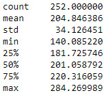
Standard Deviation

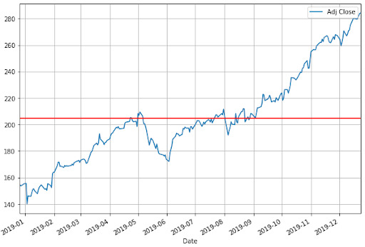
In simple words, the standard deviation tells us how far the value deviates from the mean. Let us use the full dataset and try to understand how the standard deviation helps us in the arena of trading.

We are taking into account the closing price for our calculations. As specified previously, the mean of our dataset is 204.84. The python code for Plotting the graph with the closing price and the mean should give us the following figure.

import matplotlib.pyplot as plt aapl['Adj Close'].plot(figsize=(10,7)) plt.axhline(y=mean, color='r', linestyle='-') plt.legend() plt.grid() plt.show()

The standard deviation is calculated as:

Calculate the simple average of the numbers (mean)

Subtract the mean from each number

Square the result

Calculate the average of the results

Take square root of the answer in step 4

For the data set given, the code is as follows:

std = np.std(aapl['Adj Close'])

The standard deviation of the closing price would be 34.05.

Now we will plot the above graph with one standard deviation on both sides of the mean. We will write it as (+S.D.) = 204.84 + 34.05 = 238.89, and (-S.D.) = 204.84 - 34.05 = 170.79.

The code is as follows:

aapl['Adj Close'].plot(figsize=(10,7)) plt.axhline(y=mean, color='r', linestyle='-') plt.axhline(y=mean+std, color='r', linestyle='-') plt.axhline(y=mean-std, color='r', linestyle='-') plt.legend() plt.grid() plt.show()

In the graph, the mean is shown as the middle red line while the +S.D. and -S.D. are the other red lines.

So tell us, what can you observe by looking at the above graph?

Well, a quick look tells us that most of the closing price values are in between the two standard deviations. Thus, this gives us a rough idea about the majority of the price action.

But you might still be wondering, what is the use of knowing a certain range of price values? Well, for one thing, standard deviation plays an important role in Bollinger Bands, which is a quite popular indicator. You can use the upper standard deviation as a sign of a breakout. And initiate a buy trade when the price moves above the upper band.

The volatility of the stock can be calculated using the standard deviation. The stock volatility is an important feature used in many machine learning algorithms. It is also used in Normal probability distribution, which we will cover in a while.

Wait! Normal distribution?

Normal distribution is a very simple and yet, quite profound piece in the world of statistics, actually in general life too. The basic premise is that given a range of observations, it is found that most of the values centre around the mean and within one standard deviation away from the mean. Actually, it is said that 68% of the values are within this range. If we move ahead, then we see 95% of the values within two standard deviations from the mean.

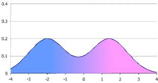
Wait, we are going ahead of ourselves now. Let us first take the help of something called the histogram to understand this.

Histogram

Let’s take an example of the heights of students in a batch. Now there might be students who have heights of 60.1 inch, 60.2 inches and so on till 60.9. Sometimes we are not looking for that level of detail and would like just to find out how many students have a height of 60 - 61 inches. Wouldn’t that make our job easier and simpler? That is exactly what a histogram does. It gives us the frequency distribution of the observed values.

When it comes to trading, we usually use the daily percentage change instead of the closing prices.

For our dataset, we will use the following code:

aapl['daily_percent_change'] = aapl['Adj Close'].pct_change() aapl.daily_percent_change.hist(figsize=(10,7)) plt.ylabel('Frequency') plt.xlabel('Daily Percentage Change') plt.show()

The output is as follows:

Recall how we said that the majority of the values are situated close to the mean. You can see it clearly in the histogram plotted above.

In fact, if we draw a line curve around the values, it would look like a bell.

We call this a bell curve, which is another name for the normal probability distribution, or normal distribution for short. You can see the majority of the values lying between the standard deviations, i.e. (+S.D.) = 239.6, and (-S.D.) = 172.64.

You might want to keep in mind that in a normal distribution, 68% of the values lie between one standard deviation and 95% of the values lie between two standard deviations. Moving further, we will say that 99.7% of the values lie between 3 standard deviations of the mean.

Normal distribution

When the distribution of your data meets certain requirements, such as symmetry around the mean and bell-shaped curve, we say your data is normally distributed.

Statistically speaking, if X is Normally distributed with mean µ and standard deviation σ, we write X∼N(µ, σ^2), where µ and σ are the parameters of the distribution.

Why is it useful to know the distribution function of your dataset?

If you know that your data sample is, say, normally distributed, you can make ‘predictions’ about your population with certain ‘confidence’.

For example, say, your data sample X represents marks obtained out of 100 in an entrance test for a sample of students. The data is normally distributed, such as X∼N(50, 102). When plotted, this data would look as follows:

If you increase the number of observations in your sample data set from 100 to 1000, this is what happens:

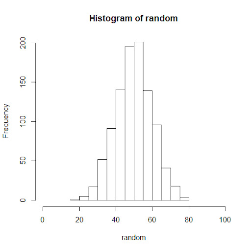
It looks more bell-shaped!

Now that we know, X has normally distributed data with mean at 50 and standard deviation of 10, we can predict the marks of the entire student population or future students (from the same population) with a certain confidence. With almost 99.7% confidence, we can say that students would not get less than 20 or greater than 80 marks. With 95% confidence, we can say that students would get marks between 30 and 70 points.

Statistically speaking, distribution functions give us the probability of expecting the value of a given observation between two points. Hence, using distribution functions, also called probability density functions, we can ‘predict’ with certain ‘confidence’.

Are closing prices normally distributed?

Before we try to answer the question, let us take another dataset and see how its histogram looks like.

We have plotted the histogram of Tesla, Inc. for the same period and see the following:

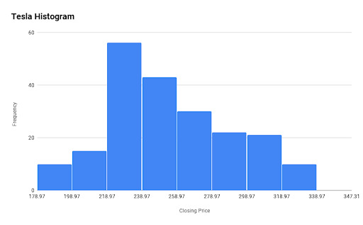
Here, the mean(Closing price) is 270.9 and the +S.D. and -S.D. is 319.14 and 222.66 respectively. So what conclusion can you draw from the above histogram?

To sum it up, probability distribution functions are used in every step of technical analysis, and it is the core of the quantitative analysis. These analyses constitute the core part of any strategy building process.

So far, we have gone through some basic concepts in the world of statistics. Now, we shall try to go a bit further in this fascinating world and see its application in trading. We will first start with correlation.

Correlation

Am I related to you or not?

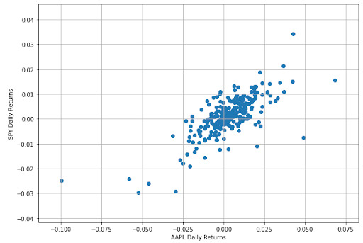
Well, in a way, correlation tells us about the relationship between two sets of values. Until now, we have taken the data set of Apple from Dec 26, 2018 to Dec 26, 2019. Now, we should point that Apple is part of the S&P 500 index. Thus, any change in Apple stocks could in some way reflect on the S&P index.

Let us take the dataset of the S&P500 for the same time period and find the correlation.

The code is as follows:

import yfinance as yf spx = yf.download('^GSPC','2018-12-26', '2019-12-26') spx['daily_percent_change'] = spx['Adj Close'].pct_change() plt.figure(figsize=(10,7)) plt.scatter(aapl.daily_percent_change,spx.daily_percent_change) plt.xlabel('AAPL Daily Returns') plt.ylabel('SPY Daily Returns') plt.grid() plt.show()

from scipy.stats import spearmanr correlation, _ = spearmanr(aapl.daily_percent_change.dropna(),spx.daily_percent_change.dropna()) print('Spearmans correlation is %.2f' % correlation)

Understanding correlation

Correlation is a unit free number lying between -1 and 1 which gives us the measurement of the relationship between variables. A highly positive correlation value lying between 0.7 and 1.0 means that the change in one variable is positively related to the change in the other variable. That means, if one variable increases, there is a high probability that other one will increase as well. The behavior will be consistent in other cases of decrease or no change in value as well.

On the other hand, a highly negative correlation value lying between -0.7 to -1.0 tells us that the change in one variable is negatively related to the change in the other variable. That means, if one variable increase, there is a high probability that the other one will decrease.

The low correlation value around -0.2 and 0.2 tells us that there is no strong relationship between the two variables.

A point to note is that correlation doesn’t tell us anything about causality. We have all heard of the statement, “Correlation doesn’t imply causation”. For instance, it is possible that instances of lung cancers are correlated with the number of cigarettes smoked in a lifetime among a population, that does not establish causality of smoking to lung cancer. One would be required to do a controlled group study keeping constant all other influential factors to establish such a causality relation. Machine learning based trading models are very good at extracting such causality between different indicators.

Correlation is the measure of the linear relationship. For instance, the correlation between x and x2 might be as close as 0. Even though there is a strong relationship between the two variables, it would not be captured in the correlation value.

Great! We have gone through a lot of concepts related to Statistics. You can move further to regression; in fact, the blog on Linear regression is a perfect next step in your quest to master the art of algorithmic trading.

Conclusion

We have gone through basic concepts of mean, median and mode and then understood the probability distribution of discrete as well as continuous variables. We looked into normal distribution in detail and touched upon the topic of correlation to figure out if two datasets are related or not.

If you want to learn various aspects of Algorithmic trading and automated trading systems, then check out the Executive Programme in Algorithmic Trading (EPAT®). The course covers training modules like Statistics & Econometrics, Financial Computing & Technology, and Algorithmic & Quantitative Trading. EPAT® equips you with the required skill sets to build a promising career in algorithmic trading. Enroll now!

Disclaimer: All data and information provided in this article are for informational purposes only. QuantInsti® makes no representations as to accuracy, completeness, currentness, suitability, or validity of any information in this article and will not be liable for any errors, omissions, or delays in this information or any losses, injuries, or damages arising from its display or use. All information is provided on an as-is basis.

Trading via QuantInsti http://bit.ly/2Zi7kP2 January 3, 2020 at 08:48AM

#IFTTT #Feedly

0 notes

maxslogic25 · 6 years

Text

PPC Divination: Forecasting Uncertainty in Excel

You’ve heard it before. Whether it’s a new idea you’re gearing up to pitch, or a request handed down to you from upper management. “Show me numbers!”

Thus, you have carefully examined and prepared data that show exactly what has happened in your accounts to-date, what’s worked and what hasn’t, and you are equipped to recommend next steps for future success. You know your account inside and out, but it’s not enough.

C-level executives spend 70% of their time thinking about and focused on the future. When they say, “show me numbers,” they aren’t talking about the numbers you already have. They want to know what the numbers are going to look like, based on the plan you’re presenting.

In an ideal world, historical data would perfectly predict future performance. Unfortunately, you work in the dynamic world of PPC, where that is rarely the case. New platform features, shifting competitive landscapes, changes in user behavior, and ever-rising prices bring a dose of unpredictability that cannot go unaddressed nor be reliably pinpointed.

Today, I’d like to share two methods of incorporating uncertainty into your PPC forecasts. You can use uncertainty variables to account for anticipated fluctuations in impression availability, CPCs, conversion rates, aggressiveness of competitors, and more.

Build Your Model

At the beginning of any uncertainty forecasting, you should first prepare your model using static numbers to test its functionality. Let’s assume, for this demonstration, that we’d like to forecast CPA for the coming quarter, anticipating a spike in our CPCs after the first of the year.

We’ll begin by identifying all the relevant metrics that will factor into our calculation. CPA is obviously the quotient of cost and conversion volume. Cost is dependent upon click volume and CPC, while conversion volume depends on clicks and conversion rate.

There are many more factors that can be included this model for added complexity (and additional layers of uncertainty accounted for), but because we are examining the impact of rising CPCs on our CPA, we will focus on only these metrics:

Clicks

CPC

Cost

Conversion Rate

CPA

Building upon the relationship between these metrics, we establish the following model to calculate CPA based on given values for all other fields and verify the logic with placeholder values.

Next, we will determine the correct values for the “constants” in our model (Clicks and Conversion Rate) by examining historical data. We find by looking at QoQ data from recent years past that Q1 tends to generate 21% more clicks than Q4 of the preceding year and conversion rates tend to be 14% higher (all else constant). Combining this information with actual data from Q4 present-year, we get forecasted values for Clicks and CVR to insert into our model.

We now have two static cells, one supporting formula cell, one output cell, and one uncertainty cell. It’s time to see how changes to the uncertainty cell impact the output cell.

Uncertainty with Discrete Probability

Let’s say that, looking at historical data, we determine there is a 15% likelihood of CPCs remaining steady QoQ at $12.35, a 45% likelihood of CPCs increasing by 7% QoQ, a 30% chance of a 12% increase QoQ, and 10% chance of an increase in CPCs equal to 17%.

We take this information to create a discrete probability table and a list of “lower threshold” values that show the cumulative sum of probabilities.

We can now update the placeholder value in our uncertainty cell (CPC) to find the Expected CPC associated with any random number between 0 and 1 according to the “lower threshold” column in our probability table.

This formula will perpetually refresh with each keystroke or press of F9 (depending on Calculation Options you have set). With each iteration of the random variable, your CPC forecast will fluctuate between the values in your discrete probability table.

Uncertainty with Normal Distribution

Now, assume that we are not able to establish a discrete probability table, but rather want to assume that possible CPC values are normally distributed with a defined mean and standard deviation (Mean and standard deviation can be found by looking at CPCs on a daily, weekly, or monthly basis for some amount of time and using the =AVERAGE() and =STDEV() functions in Excel).

In this instance, we find a mean of $13.46 and standard deviation of $.90. To find out expected CPC, we need merely use the =NORMINV function in excel, replacing the desired probability value with a random variable.

This formula will generate a random number between 0 and 1, and identify what value corresponds to that probability on a normal curve with the designated mean and standard deviation.

Iterate and Evaluate

Now that we have our uncertainty variable in place (whichever method you opted to use), it’s time to track multiple iterations of the possible outcome and evaluate with statistics. The quickest and easiest way to do this is with a data table.

First, we will create a numbered row for each desired iteration (e.g. 1000 rows for 1000 iterations—Fill Series is a great feature to help with this). In the cell directly above and to the right of “1”, we will reference our output cell (in this case, CPA).

We then use the What-If Analysis feature to create a single-variable data table, leaving the row input cell blank and selecting ANY EMPTY CELL for the column input cell.

This will iterate the random variable the specified number of times, providing a pool of possible output values according to the probability criteria you established. Taking the mean, standard deviation, min and max values of the output values in this table will give you an approximation (and understanding of likely fluctuation) of actual CPAs for the upcoming quarter given anticipated but uncertain increases in CPC.

Closing Thoughts

The method outlined above, though a simplistic example in many ways, provides a foundation for incorporating uncertainty into your forecasting models. While the world of PPC is enthusiastically data-driven, we also know that it is oftentimes unpredictable. Learning how to account for unexpected shifts will strengthen our forecasts and make it easier to move forward with confidence in our digital strategies.

It is true, there may never be a true “crystal ball” for anticipating future account performance, but a well-constructed model and a handful of uncertainty variables can certainly help us get close.

from RSSMix.com Mix ID 8217493 https://www.ppchero.com/ppc-divination-forecasting-uncertainty-in-excel/

0 notes

archiebwoollard · 6 years

Text

PPC Divination: Forecasting Uncertainty in Excel

You’ve heard it before. Whether it’s a new idea you’re gearing up to pitch, or a request handed down to you from upper management. “Show me numbers!”

Build Your Model

Clicks

CPC

Cost

Conversion Rate

CPA

Building upon the relationship between these metrics, we establish the following model to calculate CPA based on given values for all other fields and verify the logic with placeholder values.

We now have two static cells, one supporting formula cell, one output cell, and one uncertainty cell. It’s time to see how changes to the uncertainty cell impact the output cell.

Uncertainty with Discrete Probability

We take this information to create a discrete probability table and a list of “lower threshold” values that show the cumulative sum of probabilities.

Uncertainty with Normal Distribution

This formula will generate a random number between 0 and 1, and identify what value corresponds to that probability on a normal curve with the designated mean and standard deviation.

Iterate and Evaluate

We then use the What-If Analysis feature to create a single-variable data table, leaving the row input cell blank and selecting ANY EMPTY CELL for the column input cell.

Closing Thoughts

from RSSMix.com Mix ID 8217493 https://www.ppchero.com/ppc-divination-forecasting-uncertainty-in-excel/

0 notes

zacdhaenkeau · 6 years

Text

PPC Divination: Forecasting Uncertainty in Excel

You’ve heard it before. Whether it’s a new idea you’re gearing up to pitch, or a request handed down to you from upper management. “Show me numbers!”

Build Your Model

Clicks

CPC

Cost

Conversion Rate

CPA

Building upon the relationship between these metrics, we establish the following model to calculate CPA based on given values for all other fields and verify the logic with placeholder values.

We now have two static cells, one supporting formula cell, one output cell, and one uncertainty cell. It’s time to see how changes to the uncertainty cell impact the output cell.

Uncertainty with Discrete Probability

We take this information to create a discrete probability table and a list of “lower threshold” values that show the cumulative sum of probabilities.

Uncertainty with Normal Distribution

This formula will generate a random number between 0 and 1, and identify what value corresponds to that probability on a normal curve with the designated mean and standard deviation.

Iterate and Evaluate

We then use the What-If Analysis feature to create a single-variable data table, leaving the row input cell blank and selecting ANY EMPTY CELL for the column input cell.

Closing Thoughts

from RSSMix.com Mix ID 8217493 https://www.ppchero.com/ppc-divination-forecasting-uncertainty-in-excel/

0 notes

a-zhomework · 6 years

Text

Business Mathematics Amity 1st Sem

Business Mathematics 1st Amity Solution

You can buy amity solved assignments from atozhomework.com. We are honest, genuine and managed organization by a team. Post Math Homework and Get Solution Step-by-Step Join Membership and study complete document Q1: Define a subgroup. Q2: Define complete Graph with the help of examples. Q3: Explain De Morgan’s Law with examples. Q4: Explain Tautology with examples. Q5: Consider the following sample of data. 7, -5, -8, 7, 9, 12, 0, 3, 11, 8, 6, -2, 4, 10 Answer the following questions. a. What are the mean and median for this dataset? b. What are the standard deviation and variance? c. What is the range? Amity Case Study Solution "In a survey of 200 students of a College it was found that 120 had laptop, 90 had calculator and 70 had mobile phone, 40 had laptop and calculator, 30 had calculator and mobile phone, 50 had mobile phone and laptop and 20 had none of these gadgets. On the basis of above information answer the following questions. Q1. Find the number of students of calculator and mobile phone but not laptop. Q2: Find the number of students of laptop and mobile phone but not calculator. Q3: How many students have no laptop? Amity Assignment – C QUESTION 1: The complement of the union of two sets is the intersection of their complements and the complement of the intersection of two sets is the union of their complements.These are called. a. Union laws b. De Morgan s laws c. Associative laws d. Commutative laws QUESTION 2: Less than Ogive and more than Ogive intersect at a. Mode b. Mean c. Median d. Lower Quartile QUESTION 3: A terminal node in a binary tree is called........... a. Root b. Leaf c. Child d. Branch QUESTION 4: "The intersection of the sets {1, 2, 5} and {1, 2, 6} is the set ___________." a. "{1,2}" b. "{1,2,5}" c. "{1,2,6}" d. "{1,2,5,6}" QUESTION 5: Mode of a distribution can be obtained from a. Frequency polygon b. Histogram c. Less than type Ogives d. More than type Ogives QUESTION 6: Harmonic Mean is useful to find a. Average speed b. Average increment c. Average height d. None of these QUESTION 7: The set of all real numbers under the usual multiplication operation is not a group since a. multiplication is not a binary operation b. zero has no inverse c. multiplication is not associative d. identity element does not exist QUESTION 8: "Let p:7 is not greater than 4 and q : Paris is in France be two statements. Then, ~(p ? q) is the statement" a. 7 is greater than 4 or Paris is in France b. 7 is not greater than 4 and Paris is not in France c. 7 is not greater than 4 and Paris is in France d. 7 is greater than 4 and Paris is not in France QUESTION 9: Binary trees with threads are called as ....... a. Threaded trees b. Pointer trees c. Special trees d. Special pointer trees QUESTION 10: { - 3 n : n ? Z } IS an abelian group under a. subtraction b. division c. multiplication d. addition QUESTION 11: "If p: Sohan is tall, q: Sohan is handsome, then the statement Sohan is tall or he is short and handsome can be written symbolically as" a. p ?(~p ?q) b. p ?(~p ?q) c. p ?(p ?~q) d. ~p ?(~p ?~q) QUESTION 12: Mode in a asymmetrical distribution is a. Mode = 2Median-3Mean b. Mode= Median-3Mean c. Mode = 2Median-Mean d. Mode = 3Median-2Mean QUESTION 13: "Standard deviation of series 201,201,201,201,201 is" a. 201 b. 101 c. 0 d. 1 QUESTION 14: Trees are said .......... if they are similar and have same contents at corresponding nodes. a. Carbon copy b. Replica c. Copies d. Duplicate QUESTION 15: "If (G, .) is a group, such that (ab)2 = a2 b2 ? a, b ? G, then G is a/an" a. commutative semi group b. abelian group c. non-abelian group d. none of these QUESTION 16: "A={A,S,S,A,S,S,I,N,A,T,I,O,N}, B={P,O,S,S,E,S,S,I,O,N} , Find A?B" a. "S,S,S,S,I,O,N" b. "S,S,S,I,O,N" c. "I,O,N,I,S,S" d. "S,S,S,I,I,O,N" QUESTION 17: " Range of 10,20,30,40,50.60 is " a. 40 b. 30 c. 20 d. 50 QUESTION 18: Two finite sets have m and n elements. The total number of subsets of the first set is 56 more than the total number of subsets of the second set. The values of m and n are respectively a. "6,3" b. " 8,5" c. "4,1" d. " 5,5" QUESTION 19: "Median of 4,6,7,8,11 is" a. 6 b. 7.5 c. 8 d. 7 QUESTION 20: A connected graph T without any cycles is called a. free graph b. circular graph c. non cycle graph d. none of these QUESTION 21: The best measure of dispersion is a. Range b. Mean deviation c. Standard deviation d. Inter Quartile Range QUESTION 22: Two sets are called disjoint if there _____________ is the empty set. a. Union b. Difference c. Intersection d. Complement QUESTION 23: Mode of a distribution can be obtained from a. Frequency polygon b. Histogram c. Less than type Ogives d. More than type Ogives QUESTION 24: Which of the following statements is a tautology a. (~ q ?p) ?(p ?~p) b. ((~q) ?p) ?q c. (~q ?p) ?(p ?~p) d. (p ?q) ?(~(p ?q)) QUESTION 25: Which of the following is a statement? a. Open the door b. Do your homework c. Switch on the fan d. Two plus two is four QUESTION 26: "If a, b are the elements of a group G, then (ba)-1?" a. a-1 b-1 b. b-1 a-1 c. a-1 b d. b-1 a amity solved assignments for mba and bba QUESTION 27: Geometric Mean is useful to find a. Average speed b. Average increment c. Average height d. Average marks QUESTION 28: " Mean of 50,9,8,7,6, is" a. 5 b. 16 c. 7 d. 6.5 QUESTION 29: Determine the total number of subsets of the following set: a. 32 b. 64 c. 128 d. 14 QUESTION 30: A monoid is always a a. A group b. a commutative group c. semi - group d. a non abelian group QUESTION 31: There are 8 students on the curling team and 12 students on the badminton team. What is the total number of students on the two teams if three students are on both teams: a. 17 b. 20 c. 4 d. 14 QUESTION 32: "If A and B are any two sets,Then A ? (A ? B) is equal to." a. B b. A c. BC d. AC QUESTION 33: "1,2,3,4,5,6,7,y,9,9 ,10, 12,14,16. From above 14 observations we find that median is 8. The value of y is" a. 7 b. 8 c. 8.5 d. 9 QUESTION 34: The set of intelligent students in a class is a. Null set b. Finite set c. Not a well defined collection d. Singleton set QUESTION 35: Marks of a student is an example of a. An attribute b. A discrete variable c. A continuous variable d. None of these QUESTION 36: " Consider the statement, If n is divisible by 30 then n is divisible by 2 and by 3 and by 5. Which of the following statements is equivalent to this statement?" a. (a) If n is not divisible by 30 then n is divisible by 2 or divisible by 3 or divisible by5 b. (b) If n is not divisible by 30 then n is not divisible by 2 or not divisible by 3 or not divisible by 5. c. (c) If n is divisible by 2 and divisible by 3 and divisible by 5 then n is divisible by 30 d. (d) If n is not divisible by 2 or not divisible by 3 or not divisible by 5 then n is not divisible by 30. QUESTION 37: Semi Inter Quartile Range is a. Q? +Q? b. Q? - Q? c. Q? /Q? d. {Q? - Q?}/2 QUESTION 38: coefficient of Range is a. {L+S/L-S} b. {L-S / L+S} c. {2L-S/S-2L} d. None of these QUESTION 39: "Standard deviation of 1,2,3,4,5,6,7 is" a. 2 b. 3 c. 4 d. 5 QUESTION 40: Which of the following is not a measure of dispersion? a. Range b. Mode c. Inter Quartile range d. Standard deviation We also provide mcq database help for online assignment and exam purpose. Contact us for more information. Read the full article

#AmitySolvedAssignments

0 notes