#It would probably require some differential equations of vector-valued functions

[mantacid]

Awful math idea: a generalization of golf into abstract vector spaces.

[raymondsecurityadventures]

Neural Network Basics

Purpose: to breach the semantic gap between humans and machines. Humans have them naturally built into our brains; we must build them within machines.

Essentially a graph structure, where each node performs a simple computation given an input and each edge carries the generated signal from one node to another. These edges may be weighted more heavily to emphasise the importance of a signal. Each node has various inputs passed into them, and if a particular threshold is reached then the activation function will output a signal and the particular node will be activated and this output will serve as the input for the next node. Our inputs, for this project, would simply be the mentioned vectors of pixel intensities at particular points. 

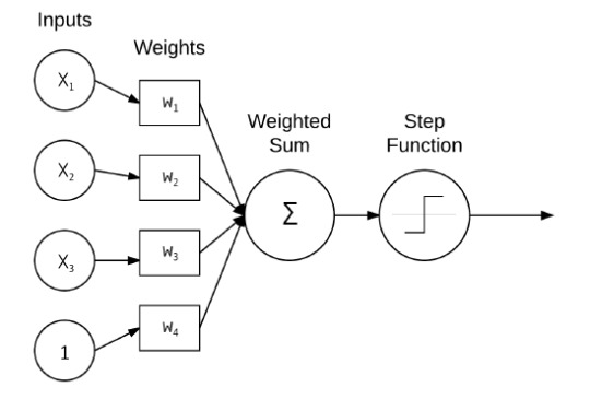
In the diagram we have a very basic NN that takes 3 inputs + a bias, and which are passed into the node to produce a weighted sum that will then be judged by the activation function to determine whether the inputs were sufficient to justify an output.

The step function before the 'signal' is sent out is meant to filter the signal - if the value is too low/signal too weak, no sendo. If it passes the threshold, yes. This is a very basic  activation function that will produce a signal if the sum reaches some threshold.

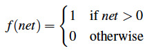
Here, our threshold is 0. If you remember your HS math, you'll know that this function is indeed not differentiable, which can lead to some issues down the line so we typically use a differentiable function as the activation function instead instead such as the sigmoid.

The sigmoid had it own issues however, so the ReLU function was born. Well, perhaps not born but came into use in NN creation.

Sigmoid (below)

ReLU (rectified linear unit) also known as a 'ramp function' and it’s equation (below)

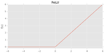
I shan't go into detail, but notice that the sigmoid's f(x) value is bound at 1 and so will  will not be able to produce any signal greater than 1 which is necessary in some NN applications. Sigmoids also take forever to compute, whilst ReLU is literally just a line.

 ReLU's cousin, the Leaky ReLU, also exists and may be used as an alternative. Which one you use really depends on your project. As the name suggests, it is a version that is leaky i.e. when input < 0, it will 'leak' a bit of signal.

The ELU (still below)

Empirically, variants of the ELU have enjoyed better performance than its cousins.   

Feedforward Network Architecture

The cornerstone of NN research, feedforward networks consist of nodes that will only feed into the next layer of nodes, never feeding backward - hence feedforward.

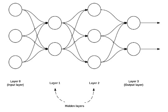
In feedforward networks, there are multiple layers, each with different functions. Layer 0 generally serves as the layer for input, where all the data enters and is processed by its nodes. Each node takes a different column/vector as an input, so for e.g. if we were training a NN to classify pictures of cats, one node may take fluffiness data and another may take tail length data.

Layers 1 and 2 in the above image serve as the layers which help process Layer 0's output and Layer 3 above is the output layer where the input data is classified into their various labels, with each node classifying a different label e.g. an NN classifying handwritten digits would have an output layer consisted of 10 nodes for each digit from 0-9 and similarly a NN classifying images of cats will simply have an output layer of a single node, which will either output 1 for yes it's a cat, or 0 for no it's not a cat.

The Perceptron Algorithm:

Not gonna go into detail since it’s not really interesting. Some believe it useful to understand. I don't.

Essentially trains a straight line of the above form to separate data belonging to two different labels by adjusting the values of that n looking symbol:

Looping over each datapoint/vector and its corresponding label

Taking the datapoint and passing it into the line function which calculates the value.

Updates each weight of the line function by the size of each step according to the output. If the output is smaller than expected, increase each weight by the step. If output is larger, decrease each weight by the step. Repeat until the line function output converges

And here’s the end product when we train the perceptron (the line that separates the data points).

Training a NN - Backpropagation:

Arguably the most important in machine learning, backpropagation is consisted of two phases:

Propagation

Backward pass

Let's look at how backpropagation and NN's work by training a NN to learn to XOR by training it on the XOR dataset which is consisted of the entire XOR domain. i.e. 0 XOR 0 is 0, 0 XOR 1 is 1 etc. etc.

Notice the dataset on the right has a third vector consisted of all 1's. This represents our bias vector and will serve as a third data vector, requiring us to add an additional input node for our NN.

Our NN will require only one single output node which will output either 1 or 0.

How deep a hidden layer should be  (recall that the hidden layers were the layers that weren't the output or input layer) is totally subjective but for easier problems like this, a single hidden layer should be fine.

After deciding on the architecture, we then must initialise the weights leading from each node. This can be done in various ways but we initialise them randomly here.

The forward pass begins which means that simply a datapoint is input into the network, and each node processes the input by multiplying it by the weights and sends a signal to the next node according to the output of the activation function. This proceeds until the output layer is reached and we are able to check its output.

If the output is lower than 0.98 and greater than 0.02, we need to apply a backward pass.

We first need to compute the error, which will simply be the difference between the predicted label and the true label of the datapoint that we're trying to predict and if you recall my earlier post, you'll remember that this error was computed using the loss function.

More specifically, we're computing the error with respect to the case, at that particular datapoint, that a particular layer were removed from the network.

We can do this by computing the partial derivative of that loss function with respect to that particular layer and multiplying the result by our step size(recall that in gradient descent we took random 'steps' blindly toward the minimal point on the loss function). If this sounds complicated, then well you'd be right, it is but luckily we don't need to understand it since we're using a high level library in Keras. If you're using Caffe, you'll probably need to know it so here's some reading. WARNING PRETTY DIFFICULT STUFF.

I should've done XXS or site injection for my project. http://neuralnetworksanddeeplearning.com/chap2.html

 Yeah so anyway after we've obtained the loss values, multiplied it with the step size we simply add this value to the weight matrix of the layer. BUT wait what’s the weight matrix of the layer? The weight matrix simply denotes the edge weights from the previous layer to the current layer, and are just an easy way to represent these edges. 

So the algorithm goes like this:

Forward pass up to the end

Find error and step size product of last layer

Add it to the weight matrix of the current layer

Iterate to the previous layer and repeat ad nauseam or until you've gotten to the input nodes

That was easy.

[learning2program]

Iterative Methods for Finding Eigenvalues

 Today, we will be reviewing some iterative methods for finding eigenvalues.

Recall that the definition of an eigenvector/eigenvalue is given some linear transformation,

\[T :  (V/F)^n \to (V/F)^n \]

then v is an eigenvector of T if T(v) is a scalar multiple of v. In other words, if we have

\[ T(v) = \lambda v, \lambda \in F. \]

Eigenvalues and eigenvectors are extremely useful in applications. For example, Google’s pagerank algorithm uses eigenvalues and eigenvectors to rank websites according to their relevance to your search. They also have uses in dynamical systems and differential equations. A good math overflow topic post about this can be found here.

In some cases, however, knowing an eigenvalue or eigenvector exactly isn’t quite that useful, since finding it generally involves using the characteristic polynomial of a matrix. Instead, in order to find quick results, it’s much more useful to estimate these things. We will be discussing the power method, the inverse iteration method, the shifted inverse iteration method, and the Rayleigh Quotient iteration method in order to find (relatively) fast estimates of eigenvalues, which will be relevant in a future project on Google’s pagerank.

In order to preform these operations, we will be utilizing the Python package SymPy for matrices. More details about this can be found here. I chose SymPy mostly just to practice with non-Numpy libraries, although Numpy can also probably be used for this. I would actually recommend that if you’re going to try to code this on your own to use Numpy, since I believe they have optimized their library using C, meaning it will be faster than what I’ve done (I have no clue if SymPy has done this, so this statement might be false). We also use the default math package.

As a preliminary, we create a norm function.

norm(vector): This function starts with a variable called norm_sq set at 0. It then iterates through all of the values of the vector, squaring them and adding them to norm_sq. It then returns the square root of norm_sq.

def norm(vector):    norm_sq = 0    for j in vector:        norm_sq += j * j    return math.pow(norm_sq, 0.5)

Power Method:

We first need to discuss a preliminary result.

Theorem: (Rayleigh Quotient) If v is an eigenvector of a matrix A, then its corresponding eigenvalue is given by

\[ \lambda =  \frac{Av \cdot v}{v \cdot v}.\]

Proof: Since v is an eigenvector of A, we know that by definition

\[Av = \lambda v \]

and we can write

\[\frac{Av \cdot v}{v \cdot v} = \frac{\lambda v \cdot v}{v \cdot v} = \frac{\lambda(v \cdot v)}{v \cdot v} = \lambda, \text{   Q.E.D.} \]

Given an n by n matrix, denoted by A, consider the case where A has n real eigenvalues such that

\[|\lambda_1| > |\lambda_2| > \cdots > |\lambda_n|. \]

Assume that A is diagonalizable. In other words, A has n linearly independent eigenvectors, denoted

\[x_1, \ldots, x_n \]

such that

\[Ax_i = \lambda_i x_i, \text{ for i = 1,..,n} \]

Suppose that we continually multiply a given vector by A, generated a sequence of vectors defined by

\[x^{(k)} = Ax^{(k-1)} = A^kx^{(0)}, \text{ }k=1,2,... \]

where 0 is given. Since A is diagonalizable, any vector in Rn is a linear combination of the eigenvectors, and therefore we can write

\[x^{(0)} = c_1x_1 + \cdots + c_nx_n. \]

We then have

\[ \lambda^k_1 \bigg[ c_1x_1 + \sum_{i=2}^nc_i\bigg( \frac{\lambda_i}{\lambda_1}\bigg)^k x_i\bigg].\]

Note that we assumed that the eigenvalues are real, distinct, and ordered by decreasing magnitude. It then follows that the coefficients of the xi’s converge to zero as we let k go to infinity. Therefore, the direction of x(k) converges to that of x1. Once we have the eigenvector from the power method, we can use the prior defined Rayleigh Quotient to find the eigenvalue as we wanted.

Using this, we then have an algorithmic way to find eigenvalues, and so we are able to code this.

powermeth(A, v, iter): Here, we have three input variables. A denotes our matrix, as should be expected by prior notation, v denotes our start vector, and iter represents the number of iterations this runs for. The function starts by running a for loop, and solving the equation

\[w = Av^{(k-1)} \]

for w. SymPy conveniently does matrix multiplication, and so all we have to do is multiply as though they were integers. We then find the norm using the norm function, as defined prior, and assign it to nor. At the end of every iteration, we find the next v vector by normalizing w (i.e. dividing tmp by nor). The function then terminates by returning the eigenvalue, which was the last value assigned to nor.

def powermeth(A, v, iter):    for i in range(iter):        #create a temporary vector to hold v^(1)        tmp = A * v        #find norm        nor = norm(tmp)        #normalize v for next iteration; i.e. v/||v||        v = tmp/nor    #returns a tuple: v is the eigenvector, nor is the eigenvalue    return nor

There are some downsides to this method, however. First off, it only finds the eigenvalue with the largest magnitude. In addition, we see that convergence is ensured if and only if all the eigenvalues are distinct. The convergence also depends on the difference of magnitude between the largest eigenvalue and second largest eigenvalue --- if they are close in size, then convergence is slow. Despite these drawbacks, though, the power method is extremely useful and still used in algorithms today.

Inverse Iteration Method:

If we have an invertible matrix, A, with real nonzero eigenvalues

\[\{\lambda_1, \ldots, \lambda_n \}, \]

then the eigenvalues of A^(-1) (A inverse) are

\[\{1/\lambda_1, \ldots, 1/\lambda_n \}. \]

In other words, by the theory of the power method, we can note this gives us the smallest eigenvalue, as opposed to the largest. The function is then as follows.

inverse_iter(A, v, iter): The requirements are the same as for the power method. The only difference is that at the start of the function, we have to calculate the inverse of A. To do this, we use SymPy’s inverse function, which uses Gaussian-Elimination to find the inverse. The process is then the same, substituting the inverse for A at each instance.

def inverse_iter(A, v, iter):    #Save time on calculation by doing the inverse first, instead of every iteration    B = A.inv()    for i in range(iter):        tmp = B * v        #find norm        nor = norm(tmp)        #normalize        v = tmp/nor    #returns the eigenvalue    return (1/nor)

The observant reader will then notice that this is a much more robust method than the prior power method. The reason for this is that we can adept this method to find any eigenvalue of the matrix, assuming we know a close estimate. Note that for any real number, the matrix

\[B = A - \mu * I \]

has eigenvalues

\[ \{\lambda_1 - \mu, \ldots, \lambda_n - \mu \}. \]

In particular, by choosing our real number to be close to the eigenvalue we want, we have that this will be the smallest eigenvalue and so by the inverse iteration method we can find it. The function is then as follows

inverse_iter_shift(A, v, estimate, iter): The difference is now we take an estimate. We start by finding I using SymPy, multiplying our estimate to I, and then subtracting I from our initial matrix A. The process is then the same as for the inverse iteration method. This is because we transformed our matrix accordingly, and so by definition the eigenvalue is also transformed.

def inverse_iter_shift(A, v, estimate, iter):    #since we asume the matrix to be square    I = sympy.eye(A.shape[0])    #Shift the matrix    B = A - I*estimate    #Invert first    B = B.inv()    for i in range(iter):        tmp = B * v        #find norm        nor = norm(tmp)        #normalize        v = tmp/nor    #returns the eigenvalue    return (1/(-nor) + estimate)

Rayleigh Quotient Iteration:

What if we could change the shift in the inverse_iter_shift function so that it adapts each iteration? We would have much faster convergence doing so. In fact, there is a method to do this using the Rayleigh Quotient Iteration. Here, we pick a starting vector, and calculate our estimate by preforming the operation

\[\lambda^{(k)} = (v^{(0)})^T A (v^{(0)}). \]

Thus, it is the same as for the inverse_iter_shift except we preform this calculation at every iteration. While more expensive, it has a cubic convergence rate as opposed to linear, and we don’t need to “know” an estimate (it depends instead on our selection of the initial vector).

RQI(A, v, iter): It essentially follows by prior, except we have to initialize a unit matrix I using SymPy to multiply with lambda. We also solve

\[(A - \lambda^{(k-1)}I)w = v^{(k-1)} \]

for w. Note that the lambda are our eigenvalues in this instance.

The code is then as follows.

def RQI(A, v, iter):    #Since we assume the matrix to be square    I = sympy.eye(A.shape[0])    for i in range(iter):        # Find lambda_0 (denote it lam)        lam = sympy.Transpose(v) * A * v        lam = lam[0]        B = A - I * lam        #If it converges, then the matrix may not be invertible (?)        try:            tmp = B.inv() * v        except:            break        #find norm        nor = norm(tmp)        #normalize        v = tmp/nor    return lam

The code can be found at the Github page, per usual. Credit to Maysum Panuj for the pseudocode inspiration.