#Raspberry Pi Compute Module serie

[androgynoustimemachineprince]

Exploring the Possibilities with Raspberry Pi: A Guide to Buying and Utilizing Raspberry Pi 4 and Its Camera Kit

Introduction:

In the world of single-board computers, Raspberry Pi stands out as a powerful and versatile option. The Raspberry Pi Foundation has continuously pushed the boundaries of what can be achieved with these compact devices. In this blog post, we will explore the benefits of Raspberry Pi 4 kit, Raspberry pi buy, and delve into the exciting projects you can undertake using this remarkable technology.

Why Choose Raspberry Pi 4 Camera? Raspberry pi 4 camera is the latest iteration of the Raspberry Pi series, offering improved performance and enhanced features. It comes equipped with a Broadcom BCM2711 quad-core Cortex-A72 processor, clocked at 1.5GHz, which ensures smooth multitasking and faster execution of complex tasks. The availability of up to 8GB of RAM allows for efficient handling of data-intensive applications. With its support for dual-band Wi-Fi and Bluetooth 5.0, Raspberry Pi 4 provides seamless connectivity options for your projects.

Exploring the Camera Capabilities: One of the most exciting features of Raspberry Pi 4 is its compatibility with a dedicated camera module. The Raspberry Pi Camera Module v2 is a high-quality camera that can be easily connected to the board via the camera interface. The camera module offers an 8-megapixel sensor and supports video resolutions up to 1080p, enabling you to capture stunning photos and videos. Its compact size and versatility make it perfect for various applications, including surveillance systems, time-lapse photography, and even computer vision projects.

Where to Buy Raspberry Pi 4 Online: When it comes to purchasing Raspberry Pi 4 and its accessories online, there are several reputable platforms to consider. Some popular options include:

Online Retailers (e.g., Amazon, Robomart, SparkFun) Established Raspberry pi buy online platforms like Amazon, Robomart, and SparkFun also stock Raspberry Pi 4 boards, camera modules, and kits. These retailers often provide customer reviews and ratings, giving you insights into the products before making a purchase.

Specialized Electronics Retailers Various specialized electronics retailers cater specifically to the Raspberry Pi community. These retailers often have a wide range of Raspberry Pi products, including kits that include the camera module.

Exciting Raspberry Pi 4 Projects: Once you have your Raspberry Pi 4 and camera kit, the possibilities for projects are virtually endless. Here are a few ideas to get you started:

Home Surveillance System: Set up a motion-activated camera system to monitor your home remotely and receive alerts on your smartphone.

Wildlife Monitoring: Create a wildlife camera trap that captures photos or videos of animals in their natural habitats.

Time-Lapse Photography: Capture the beauty of nature or the progress of a construction project by creating stunning time-lapse videos.

Facial Recognition: Develop a facial recognition system using the camera module and explore applications in security or access control.

Virtual Assistant: Transform your Raspberry Pi 4 into a voice-controlled assistant by integrating a microphone and speaker.

Conclusion: Raspberry Pi 4, along with its camera module, opens up a world of possibilities for hobbyists, educators, and professionals alike. Whether you're interested in building a smart home system or exploring computer vision applications, Raspberry Pi 4 provides the necessary power and flexibility. With numerous online platforms available to purchase Raspberry Pi 4 and its accessories,

[awerobotics]

Essential Python Techniques for Robot Motor Control

Robotics is a multidisciplinary field that merges concepts from mechanical engineering, electrical engineering, and computer science to design and build robots, machines capable of performing a series of actions either autonomously or semi-autonomously. A crucial aspect of robotics is motor control, which involves the accurate and smooth command of a robot's movements. Python, renowned for its clear syntax, extensive library support, and active community, has become a popular choice for programming in robotics, particularly for implementing Python techniques for robot motor control. It offers various libraries and modules that simplify the development and control of robots. Python's flexibility allows for quick prototyping, integration with other programming languages, and hardware devices.   Importance of Motor Control in Robotics Motor control is central to robotics. It involves directing the robot's movements, enabling it to move from one point to another, manipulate objects, or perform specific tasks. Precise motor control is essential for the robot to execute tasks accurately and efficiently. Robots typically have multiple motors that control different parts of their body, such as wheels, arms, or other actuators. Each motor must be controlled accurately to achieve coordinated movements. Python provides tools and libraries to implement sophisticated motor control algorithms. Python Techniques for Robot Motor Control Pulse Width Modulation (PWM) PWM is a technique used to control the speed and direction of motors by varying the duty cycle of a signal, which controls the power supplied to the motor. Python libraries like RPi.GPIO and Adafruit_PCA9685 generate PWM signals to control motor speed and direction. How PWM Works The duty cycle of a signal refers to the percentage of one period in which a signal is active. PWM uses digital signals to simulate analog results. By varying the duty cycle of a signal, we can change the amount of power supplied to a motor and consequently, control its speed and direction. Implementing PWM in Python To implement PWM in Python, you can use the RPi.GPIO library. This library provides a simple interface for controlling the GPIO pins of a Raspberry Pi. Below is an example of how you can use the RPi.GPIO library to generate a PWM signal and control a motor's speed and direction: In this example, the motor is connected to GPIO pin 18 of the Raspberry Pi. The PWM frequency is set to 1000 Hz, and the PWM is started with a 50% duty cycle. The motor speed is then changed by adjusting the duty cycle. Proportional-Integral-Derivative (PID) Control PID control is a closed-loop control system that continuously calculates the error between the desired and actual positions of the motor and adjusts its speed accordingly. Python has several libraries, such as simple_pid and PID, that simplify PID control algorithms implementation. How PID Works A PID controller calculates the error between the desired setpoint and the actual process variable and applies a correction based on proportional, integral, and derivative terms. The controller attempts to minimize the error over time by adjusting a control variable, such as the motor speed. Implementing PID in Python To implement a PID controller in Python, you can use the simple_pid library. This library provides a simple and easy-to-use PID controller implementation in Python. Below is an example of how you can use the simple_pid library to implement a PID controller that controls a motor's position: In this example, the setpoint is set to 100, and a PID controller is created with the specified gains. The motor_position is then controlled using the PID controller until it reaches the setpoint. Trajectory Planning Trajectory planning involves determining the path that the robot will follow to reach its destination. Python libraries like matplotlib and scipy can plot and analyze trajectories, while optimization algorithms in scipy.optimize can optimize the robot's movement. How Trajectory Planning Works Trajectory planning involves calculating the path that a robot should follow to move from its current position to a desired position while avoiding obstacles and satisfying constraints such as speed and acceleration. A trajectory can be represented as a series of waypoints that the robot should pass through. Implementing Trajectory Planning in Python To implement trajectory planning in Python, you can use the scipy library. This library provides functions for numerical integration, interpolation, optimization, and other scientific computing tasks. Below is an example of how you can use the scipy library to implement trajectory planning for a robot: In this example, a set of waypoints is defined, and a spline is fitted to the waypoints using the splprep function from scipy.interpolate. The spline is then evaluated at multiple points using the splev function, and the resulting trajectory is plotted using matplotlib. Motion Control Algorithms Motion control algorithms, such as kinematic and dynamic models, help translate desired movements into motor commands. Python libraries like sympy and pydy can help derive and solve these models. Kinematic Control Kinematic control deals with the geometric aspect of the robot's movement. It involves determining the joint parameters required to move the robot to a desired position and orientation. Kinematic control does not consider the forces and torques involved in the robot's movement. Dynamic Control Dynamic control, on the other hand, considers the forces and torques involved in the robot's movement. It involves determining the joint forces and torques required to move the robot to a desired position and orientation while satisfying constraints such as speed, acceleration, and force limits. Implementing Kinematic Control in Python To implement kinematic control in Python, you can use the sympy library. This library provides functions for symbolic mathematics, which can be used to derive and solve the kinematic equations of the robot. Below is an example of how you can use the sympy library to implement kinematic control for a robot arm with two links: In this example, the forward kinematics equations for a two-link robot arm are defined using the symbolic variables theta1, theta2, l1, and l2. The desired end-effector position x_desired and y_desired is defined, and the forward kinematics equations are solved for the joint angles theta1 and theta2. Feedforward Control Feedforward control is a strategy where the control action is calculated based on a model of the system and the desired trajectory, without using feedback from sensors. This strategy is often used in conjunction with feedback control (such as PID) to improve the system's response to disturbances. Implementing Feedforward Control in Python In Python, feedforward control can be implemented by using a model of the system to compute the control input required to follow a desired trajectory. Below is an example of how to implement feedforward control for a simple robot: In this example, the system model, desired trajectory, and feedforward control law are defined. The system is then simulated using a loop, where the control input is computed at each time step using the feedforward control law, and the state is updated using the system model. Sliding Mode Control Sliding mode control is a non-linear control strategy that aims to bring the system's state onto a predefined surface in the state space, called the sliding surface, and then keep it on this surface until the desired state is reached. This strategy is particularly useful for systems with uncertainties and external disturbances. Implementing Sliding Mode Control in Python In Python, sliding mode control can be implemented by defining the sliding surface and then designing a control law that forces the system's state onto the sliding surface. Below is an example of how to implement sliding mode control for a simple robot: In this example, the system model, sliding surface, and sliding mode control law are defined. The system is then simulated using a loop, where the sliding surface and control input are computed at each time step, and the state is updated using the system model. Optimal Control Optimal control involves finding the control input that minimizes a cost function while satisfying the system dynamics and constraints. This strategy often involves solving a mathematical optimization problem. Implementing Optimal Control in Python In Python, optimal control problems can be solved using optimization libraries such as scipy.optimize. Below is an example of how to implement optimal control for a simple robot: In this example, the system dynamics, cost function, and optimization problem are defined. The optimal control input is then computed by solving the optimization problem, and the system is simulated using a loop, where the state is updated at each time step using the system dynamics and optimal control input. Adaptive Control Adaptive control involves adjusting the control parameters in real-time based on the system's behavior and the desired trajectory. This strategy is particularly useful for systems with unknown or varying parameters. Implementing Adaptive Control in Python In Python, adaptive control can be implemented by updating the control parameters at each time step based on the system's behavior and the desired trajectory. Below is an example of how to implement adaptive control for a simple robot: Advanced Motor Control Strategies While the techniques mentioned above are fundamental and widely used, several advanced motor control strategies can be implemented using Python. Some of these include: - Model Predictive Control (MPC): This is an advanced control strategy that computes control inputs by solving an optimization problem at each time step. Python has several libraries, such as cvxpy and scipy.optimize, that can be used to implement MPC. - State Space Control: This involves representing the system as a set of first-order differential equations and designing a controller that places the poles of the system in desired locations. Python offers various tools and libraries, such as scipy.signal and control, that can be used to design and implement state-space controllers. - Neural Network Control: This involves using neural networks to model the system dynamics and design the controller. Python has several libraries, such as TensorFlow and PyTorch, that can be used to implement neural network controllers. Implementing Model Predictive Control in Python To implement MPC in Python, you can use the cvxpy library. This library provides a Python interface for defining and solving convex optimization problems. Below is an example of how you can use the cvxpy library to implement MPC for a simple robot: In this example, the system dynamics are defined by the matrices A and B, and the initial state x0 is defined. The MPC parameters N, Q, R, and x_ref are specified, and the decision variables x and u are defined. The objective function is defined as the sum of the state and control input costs over the prediction horizon N, and the system dynamics are added as constraints. The optimization problem is then defined and solved using the cvxpy library, and the optimal control input is extracted and printed. Conclusion Python offers various tools and libraries that can be utilized for robot motor control. From basic techniques such as PWM and PID control to advanced strategies such as MPC and neural network control, Python provides a versatile platform for implementing motor control algorithms for robots. Understanding these techniques and how to implement them using Python is crucial for anyone working in the field of robotics or automation. This article provides a detailed explanation and Python code examples for several motor control techniques, which can serve as a foundation for more advanced applications. Key Takeaways - Python is a versatile language for robot motor control: With its clear syntax, extensive library support, and active community, Python is an excellent choice for implementing motor control algorithms for robots. - Basic motor control techniques are essential: Techniques such as PWM, PID control, and trajectory planning are fundamental and widely used in robotics. Understanding these techniques and how to implement them using Python is crucial for anyone working in the field of robotics or automation. - Advanced motor control strategies can be implemented using Python: Python offers various tools and libraries that can be used to implement advanced motor control strategies such as MPC, state-space control, and neural network control. Note that this is a general guide, and the specific implementation might vary based on the robot's hardware and software configurations. Additionally, always ensure the safety of yourself and others when testing and implementing motor control algorithms on real robots. This guide has provided you with the foundational knowledge and practical skills required to implement Python techniques for robot motor control. Understanding and implementing these techniques is crucial for anyone working in the field of robotics or automation. Whether you are a student, a hobbyist, or a professional, mastering these techniques will equip you with the necessary skills to develop and control robots using Python. Remember to continuously test and optimize your code to ensure that the robot operates efficiently and safely. Also, it is essential to stay updated with the latest developments in the field of robotics and Python programming as new tools and techniques are continually being developed. Disclaimer: The examples provided in this article are for educational purposes only and should be used with caution. Always ensure the safety of yourself and others when testing and implementing motor control algorithms on real robots. Read the full article

[idein-inc]

Why RaspberryPi VC4 GPGPU Programming Matters

Written by: Noriyuki Ohkawa Translated by: Ryohei Tokuda

This article is the English translation from https://blog.idein.jp/post/185103625470/whyvc4matters.

The Raspberry Pi series uses a GPU called VideoCore IV (VC4) to render on display. Displaying is not necessary in most cases if we use Raspberry Pis as sensing devices. Therefore we use vacant VC4C to accelerate deep-learning inferences.

The advantages of GPGPU on VC4 are the following three:

Easy to share programs between products

Available CPU for other tasks

Less affected by over-heating

Easy to share programs between products

All of Raspberry Pi models, from pi0 to pi3, have VC4 although the frequency differs: 250MHz or 300MHz. We can say VC4 is the central unit because VC4 is initially booted, and then VC4 will kick the board's CPU.

Though all the GPUs have similar performance, the performances of CPU of pi0 and pi3 are very different. Although pi3 works fine for a substantial inference task using CPU, pi0 may not be able to execute the same program. Pi3 has SIMD ALU, but pi0 doesn't. This means we need to prepare different programs for pi0 and pi3.

In contrast, the inference performance by VC4 is almost constant. Therefore we can share the same program between the different products. We use the same program for our Actcast (currently alpha) demo program for different Raspberry Pis.

Available CPU for other tasks

On deep-learning sensing tasks, inference in itself is only one part of an application: for real applications, additional tasks such as taking a photo, pre-process, post-process, displaying (if necessary), or sending data are required. Inference by CPU exploits almost all of the CPU capacity, even though pi3 has four cores. Therefore the throughput cannot be increased.

Inference by VC4C doesn't use CPU at all. Therefore task parallel using CPU and VC4 increases the throughput by pipelining inference tasks and other tasks.

Less affected by over-heating

Pi3's CPU is powerful: if you can design and train it, a small Neural Network inference should run with the same speed on one CPU core as a VC4 version.

Theoretically, the four CPU cores are faster than VC4. For this reason, we have developed a converter to generate codes for not only VC4 but also CPU as MISRA-C.

Here we show the example of segmentation to make person-part blue. First by VC4:

Next by a CPU core of the same model:

The same model by two CPU cores:

The same model by three CPU cores:

Although we can optimize performance using multiple CPU cores by pipelining and assigning tasks to each core, execution by more than two CPU cores produces much heat. By default, the frequency of CPU cores is diminished if the temperature exceeds 80 °C. Over 85 °C, the frequency is halved. Hence the use of multiple CPU cores doesn't make speed-up without heat countermeasures. Of course, inference and other tasks by CPU cores are affected by its heat throttling.

For real operation, heat countermeasures are troublesome: driving parts such as fans are easily affected and injured by dust. A heat-sink such as metal case is desirable if it can do enough heat-release. The following picture is pi3 with a metal case. Without it, inference by CPU cores is soon affected by over-heat.

It might be interesting to check heat-design, temperature guarantee of recent "special chips" or Raspberry Pi like boards, and how the guarantee is archived.

As described above, the CPU thermal throttling starts at 80 °C, whereas the VC4 thermal throttling begins at the (relatively high) temperature of 85 °C. If the chip becomes hot during inference using VC4, CPU thermal throttling begins at first to suppress heating of the chip. For most applications, the inference (run on GPU) is the bottleneck, so thanks to the above mentioned pipelining between CPU and GPU, even if side tasks (run on CPU) spend more time than before over-heat, the overall execution time is unchanged. This is the reason why we do our demonstrations without metal cases, heat sink, or fans in exhibits.

Of course, if we pack pi0 or pi3 into a close-to-be-sealed container, like plastic cases, we can observe speed-down even with VC4. For the same reason, a Compute Module is little room for heat dissipation. Therefore, careful heat design is required.

Summary

Inference by VC4 has many advantages in addition to its speed.

For deep-learning acceleration boards, one naturally tends to focus on speed. However, for real operations, the choice of edge devices requires several considerations: costs including heat countermeasure, the ease of making applications, etc.

[zenatixsolutions]

IoT Powered Building Management System for Small and Medium Sized Buildings

Building Management Systems (BMS) have been used to automate equipment in large buildings for almost 3 decades, but such systems are not suitable for small and medium sized buildings (of less than 100K sq. ft.). This problem is compounded by the fact that customer’s multiple locations are dispersed across the geography, making it difficult to drive consistent manual behaviour, resulting in challenges such as high energy costs, compliance issues, and asset breakdown.

IoT powered building management system for small and medium sized buildings helps in optimizing energy consumption, maintaining temperature compliances, managing asset health and facilitating digital workflows. It works across protocols and equipment of multiple OEMs. The technology is wireless, plug & play enabling easy deployments and maintenance. Being a hardware light solution, it is cost-effective and delivers a faster return on investment.

IoT Technology that fulfills SMB needs

It’s not easy for small and medium-sized buildings (SMB) to invest a massive sum of money to ensure efficient operations. The Internet of Things (IoT) is a powerful technology that focuses on in-house innovations across edge devices & their networking, cloud platforms, and end-user interfaces. Ensuring building productivity, optimal energy consumption, and automation at reduced cost becomes possible with this smart technology.

The Internet of Things (IoT) comes with:

Wireless Mesh for Sensing and Control

An open-source wireless mesh OpenThread (from Google) develops a mesh-based robust solution that includes a wide variety of battery-powered sensors such as temperature, humidity, luminosity, CO2, etc. It relays data to a gateway using multiple hops on the mesh network.

The whole network is resilient to faults and opens up a broad variety of applications ranging from deploying a large number of sensors inside/outside buildings within a campus to connected street lighting solutions spread across a large municipality.

Industrial Grade Gateway

IoT often comes in a state-of-the-art gateway that is an open platform based on Raspberry Pi Compute Module (contains a 32-bit Quad-core processor, 1GB RAM, and onboard disk, and operates on a Linux-based Operating system). It supports a wide variety of connectivity options through the plug & play modules such as 4G through an mPCIE card, WiFi/Bluetooth/OpenThread through an M.2 card, and onboard LAN.

The IoT gateway supports multiple features for rugged operation in difficult environments in small and medium-sized buildings, including dual SIM connectivity, battery-backed RTC, onboard watchdog, battery backup, and isolated RS485 connectivity.

IoT Stack on Cloud

Cloud-connected IoT stack developed using open-source technologies delivers standard services such as alerts, time series databases, reports, and dashboards.

This integrated analytical platform provides scalability to small and medium-sized buildings. The configurable dashboard platform allows facility managers to customize different user interfaces across and within the customer through drag-and-drop elements without writing a single line of code.

Choosing a cloud-based IoT stack means managing more than 200 Mn data points every single day that can scale up to 100X very easily.

Plug & Play Platform

Typical deployment timelines in buildings and chains are a bit long (actually depends on the sq. ft area). On-site hardware systems consisting of the industrial-grade gateway and sensing/control endpoints on the multi-hope, wireless mesh enable faster deployment, bringing down the timeline of legacy hardware by 50-80%.

This plug-and-play platform enables remote deployment, troubleshooting, and maintenance of the edge hardware.

Is a small size building actually worth a BMS?

Well, the honest answer is “no.” Building management systems haven’t been designed for small buildings. The ideal solution is the implementation of IoT BMS, which is cost effective and ROI based solution.

Get Zenatix IoT BMS For Your Small And Medium Size Buildings Now!

Zenatix’s powerful IoT-based solutions can help you implement the right BMS for your small and mid-size buildings. Get in touch with us today!

View Source : https://www.zenatix.com/iot-powered-building-management-system-for-small-and-medium-sized-buildings/

[ktdrita]

Focuswriter raspberry pi

#Focuswriter raspberry pi how to#

Maybe lower speeds would be a little more stable? The Raspberry Pi RP2040 microcontroller chip is designed to run at 133 MHz, but it CAN be overclocked to run as high as 1 GHz… it’s just unlikely to survive for more than a few minutes in that state. Here’s a roundup of recent tech news from around the web. The results are both impressive and potentially destructive. In other Raspberry Pi-related news, there’s a new adapter that lets you use a Raspberry Pi Zero as if it were a Raspberry Pi Compute Module 3, and a Raspberry Pi intern wanted to find out what happened if you overclocked a RP2040. Performance comparison of 7 tiny PC boards including Raspberry Pi Zero and Zero 2W and similarly-sized models with ARM-based chips from Allwinner or Amlogic, plus the MangoPi MQ Pro with an Allwinner D1 RISC-V processor. And Bret Weber has managed to assemble a bunch of them and run a series of performance tests that may help you decide which best meets your needs. But there are also a growing number of other tiny PCs competing in this space. The Raspberry Pi Zero and Raspberry Pi Zero 2 are incredibly small, cheap, and versatile single-board computers… but in a time of global supply chain shortages, they’re also kind of hard to get your hands on these days.

How long will my Fire Tablet get security updates?.

#Focuswriter raspberry pi how to#

How to use an SD card with Amazon’s Fire tablets.How to sideload apps on Amazon Fire tablets.How to disable Amazon apps and features.Hack your Amazon Fire tablet with Fire Toolbox.How to install Google Play on the Amazon Fire HD 10 (9th-gen).How to install Google Play on the Amazon Fire HD 8 (2020).How to install Google Play on the Amazon Fire 7 (2022) with Fire OS 8.Lilbits: Raspberry Pi Zero-like mini PCs compared, RP2040 microcontroller overclocked, and reducing the wait time for Purism's Librem 5 Linux smartphones - Liliputing Close Search for: Search

[techcree]

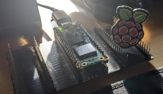
Raspberry Pi und Raspbi PicoW + Sensoren (1/2)

Heute geht es vor alle um ein Paar Sensoren. Es geht aber auch darum wie passen diese zum Repaberry Pi Pico oder muss doch der Raspberry Pi dafür her.

Nach dem großen Erfolg des Microcontrollers der Raspberry Pi Foundation UK, dem Pico, hat Raspberry nochmal nachgelegt und den PicoW auf den Markt gebracht. Der ist nun gegenüber dem Bruder mit einem WLAn Modul ausgestattet. Gleich vorweg, es wird zu diesem Bericht noch einen zweiten Teil geben, denn aktuell liegt noach nicht alles Material zum Test vor. Allerding ist nun der Pico W auch bei mir eingetroffen und auch einer der Sensor-Module ist da. Konkret handelt es sich um den BME688.

Natürlich sind die Erwartungshaltungen an den neuen PicoW hoch. Hinsichtlich seiner Anschaffungskosten liegt der nur geringfügig über dem Vorgänger, wo bei der Pico im Vergleich zum PicoW ja eigentlich kein Vorgänger im eigentlichen Sinne ist, denn es gibt aj noch beide im Handel. Das Beide ihre Käuferschicht haben, also auch der Pico weiterhin gefragt sein wird, dass jedenfalls dürfte niemand bestreitet. Es ist also nicht so das der PicoW den Pico quasi ablösen wird.

Warum? Ein WLAN Modul an Board ist grundsätzlich eine feine Sache und damit zieht Raspberry technologisch Modellen der Mitbewerber nach. Doch was bringt uns diese WLAN Funktionalität an Mehrwert. Wie sinnvoll lässt sich der PicoW also wirklich für unsere Projkete einsetzen bzw. auch für alltagstaugliche Lösungen einsetzen? Dazu später mehr.

Hinweis: Beitrag enthält kostenlose und unbezahlte Werbung. Bildquellen unter anderem: pimoroni.com

Kommen wir zuvor zu den Sensor Modulen, den sogenannten Sensor Breakouts. Ich habe mir den BME688 und den BME280 Sensor bei Pimoroni bestellt und leider nicht darauf geachtet alles in eine bestellung zu packen. Daher lieferte Pimoroni wie gewohnt schnell und zuverlässig den PicoW nebst dem in dieser Bestellung enthaltenen BME688. Aber kein Problem über den Test des BME280 erfahrt Ihr dann mehr im zweiten Teil.

Aber was sind das eigentlich für Sensoren? Im Prinzip unterscheiden sich diese Breakouts nur im Hinblick auf das was alles gemessen werden kann. Während beim BME280 Luftdruck, Temperatur und Luftfeuchtigkeit gemessen werden können sind die BME68X noch in der Lage die Luftqualität (Gas) zu messen. Gehen wir an dieser Stelle noch nicht darauf ein was es uns bringen mag diese Daten zu erhalten, also diese Dinge zu messen. Auch das noch später.

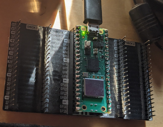
Zunächst schließen wir den Raspberry Pi PicoW wie bereits vom Pico gewohnt am Computer an und betanken den Microcontroller mit der passenden .UF2 Datei, um dann Micropython als Programmiercode nutzen zu können. Und um die dann auf dem PicoW zu speichern und den Code zu bearbeiten verwende ich auch hier die ThonnyIDE. Aber das hier gibt kein Tutorial, daher bitte detailierte Anweisungen dazu selbst nachschauen. An der Stelle merken wir jedenfalls kaum einen Unterschied zum Pico außer das wir nun eine für den PicoW geeignete .UF2 benutzen müssen.

Was uns der PicoW aber jetzt bietet, ist bspw. unter der Verwendung der Phew Bibliothek einen Mini-Webserver darauf laufen lassen zu können. Neben Phew bieten sich natürlich auch noch andere Wege an. Ich habe mich aber für Phew entschieden um den reinen .html Code als eigene index.html Datei bearbeiten zu können. Den Webserver zu starten und zu betreiben hat sich damit als deutlich stabiler und unkomplizierter erwiesen.

Um sich nun auf einer Website bspw. einmalig die Temperatur anzeigen zu lassen, die der PicoW messen kann ist erstmal kein Breakout Sensor wie der BME280 erfolrderlich! Der Pico verfügt auf der Platine bereits über einen Temperatursensor ebenso wie über eine LED. Wollen wir aber mehr messen, dann empfiehlt sich hier eben der BME280. Warum der und nicht die Sensoren der 68x Serie? Aktuell gibt es für Micropython nur eine BME280_micropython Bilbliothek, welche wir auf dem Pico und PicoW erfolgreich istanllieren können! Ja, pech das ich gerade zum Start neben dem PicoW den 688'er geliefert bekam.

Ein Tipp den ich euch auf jedenfall noch geben möchte ist es die Informatioen über euer WLAN, wie die SSID und das Passwort nicht direkt in die main.py Datei zu packen, sondern eine eigene secrets.py damit zu erstellen. Die Daten für die Anmeldung im WLAN zieht ihr euch dann dort einfach heraus mit "from secrets import SSID, password". Ist der Webserver gestartet ist die .html-Seite unter der IP Adresse im Browser aufrufbar, welche euer Router dem PicoW vergeben hat. Bekommt ihr natürlich nach dem Start der main.py im ThonnyIDE auch angezeigt.

Kommen wir auf den BME688 zu sprechen. Es gibt von der Software oder auch dem Python Code zwischen dem BME680 und dem BME688 keinen auffäööigen Unterschied. Ob ihr euch nun für den 680'er oder den 688'er entscheidet müsst ihr selbst mal nachlesen. Die beiden Sensor breakouts sind auf der Website von Pimoroni gut beschrieben und unterscheiden sich vor allem im Preis. Sprechen wir über diesen Sensor fällt uns auf, dass hier BOSCH die Finger im Spiel hat. BOSCH bietet dazu auch eine Auswertungssoftware. Die läuft aber nur als APP Version und kann wiederum auf dem Raspberry Pi 4 bei mir nicht ohne Umwege laufen.

Die Daten des BME688 bekomme ich aber eben super auf dem Raspberry Pi Einplatinencomputer erfasst und angezeigt. Die Installation des BME688 ist bei meinem Pi4 ziemlich einfach gewesen. GPIO Schnittstelle muss natürlich aktiviert sein. In der ThonnyIDE die entsprechenden Bibliothkenen für Python zu finden und zu installieren iat auch kein Hexenwerk. Zudem bietet genau hier an dem Punkt Pimoroni ein umfangreices Tutorial an, welches ihr auf deren Seiten findet. Über die Pimoroni GitHub Page gibt es zudem eine detailierte Installationsanleitung und ein Installationsscript.

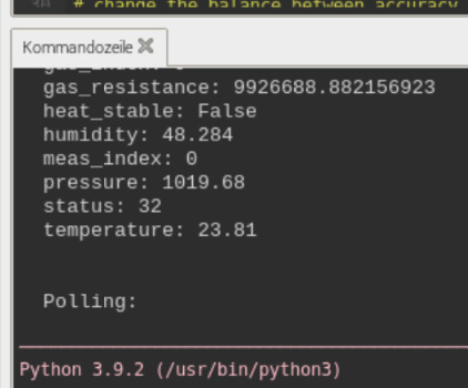
Die passenden Demo Scripte gibt es dann auch driekt mit. An der Stelle hat Pimoroni wiedermal einen klasse Job gemacht! Vielen Dank nach GB an Pimoroni dafür! Läuft das Script dann gibt es Daten, Daten, Daten. Nun was die Temperatur dabei aussagt ist uns allen wohl klar. Auch beim Luftdruck und der Luftfeuchtigkeit kommen wir sicher noch hin. Was uns der gas_resistance Wert aber sagt müssen wir ggf. nachforschen. Es sei denn man kennt diese Werte und kann damit umgehen. Der Laie, der aber zum ersten Mal diesen Wert sieht wird sicher zunächst etwas staunen.

Warum spreche ich das an? Na klar! Es gibt bei BOSCH eine sehr umfangreiche Beschreibung zu diesem Sensor. Diese kann man sich dort von der Website als *.pdf Dokument herunterladen. Und ja bevor ich euch das alles verlinke. Den Job hat auch Pimoroni bereits für uns gemacht.

Also einen Link hier für alle Infos die Ihr so benötigt: https://shop.pimoroni.com/collections/electronics

So und bevor dieser Beitrag schlicht zu lang wird vertröste ich euch nun an dieser Stelle auf den bald folgenden zweiten Teil. Dann auch mehr zum BME280!

[cardfox19]

General Touch Driver

Download Generic PnP Monitor Drivers - Install and Update.

General Touch Touch 232 input device drivers | Download for.

Generic Silead touch driver for Windows 10 ? | XDA Forums.

Fusion5 Tablet Touch Screen - Windows 10 Forums.

吉锐触摸 - General Touch.

REFInd / Discussion / General Discussion: Touchscreen is.

Download - General Touch Co., Ltd.

TouchKit USB Controller for TouchScreen - Free download.

Touch Driver.

Latest Windows 8 & 8.1 Drivers (September 21, 2021).

Download General Touch drivers for Windows 7, XP, 10, 11, 8.

General availability: CSI storage driver support on Azure.

Fix Generic PnP Monitor Issue in Windows 10 (Easy Guide).

EloTouch Solution | Support | Driver Download.

Download Generic PnP Monitor Drivers - Install and Update.

Most manufacturers regularly release driver updates for their hardware that are specifically designed for this version of Windows. Below is a list of information on Windows 8 drivers and general compatibility information for major hardware and computer system makers, including Acer, Dell, Sony, NVIDIA, AMD, and much more. Method 2: Download and Install Generic Bluetooth Radio Driver From Manufacturer's Official Page. You can use the manufacturer's official website to update the Bluetooth driver.It is a manual approach to perform the driver updates, so be sure that you have proper time, technical expertise, and a lot of patience. Touch Screen Driver free download - Don't Touch My Computer Episode 2, CopyTrans Drivers Installer, nVidia 3D Stereo Driver (Windows 2000/XP), and many more programs.

General Touch Touch 232 input device drivers | Download for.

This self-extracting zip file contains the driver for the driver for the TouchKit Touchscreen. It enables the features and functions of the touchscreen. How to extract the files: - Download the self-extracting EXE zip file from the website to a directory on your hard drive. - Run the downloaded file to extract the driver files. Touch Screen Drivers. Since updating my DELL Inspiron 15R from Windows 8.1 to Windows 10 the Touch Screen has stopped working. Selecting 'Device Manager>Human Interface Devices' reveals that the 5 icons (which can only be seen by using 'View>Show hidden devices) for 'HID-compliant....' are greyed out - device, touch screen, defined device (x3. Actually to add, the driver does claim that this touchscreen is an egalax touchscreen. So the driver is definitely the closest step so far. I may have just configured something wrong, but I am not sure what. There is no Touch Screen device in device manager, but the driver does come up with this.

Generic Silead touch driver for Windows 10 ? | XDA Forums.

So far I've tried 2 different drivers I've found online. The first is the UPDD 4.1.8 from this website but it didn't include the correct driver so didn't work. The second one I tried was from this website and was the first one listed under Windows 7 (5.12.0.11912). It installed the correct driver but I couldn't get the touchscreen adequately. Download General Touch drivers or install DriverPack Solution software for driver scan and update. Download Download DriverPack Online. Find. General Touch devices.

Fusion5 Tablet Touch Screen - Windows 10 Forums.

If there is a yellow exclamation mark next to the entry, right click on it and select the Update Driver Software and follow the prompt Search Automatically for Updated Driver Software. This should find and install the driver software for your Touchscreen. UPDATE 30/09/2016. Hi, @Shantel Brassfield,. DMT should be selected for general computer monitors. The following table shows the resolution options commonly used for external HDMI monitors: Note: The common 7-inch Raspberry Pi touch module on the market has a resolution of 1024x600.

吉锐触摸 - General Touch.

Jan 07, 2019 · DMC TSC-Series DMT-DD Win10. 15.02.2019. 2.05. Filesize: 13MB. *4. *1 If the driver is to be used on Windows XP, either.Net Framework 2.0, 3.0. or 3.5 need to be installed on your PC. *2 If the driver is to be used on Windows XP, use this version if one of.Net. Framework 2.0, 3.0, or 3.5 are not installed on your PC. Jul 03, 2020 · How to download touch screen driver for Windows 10? Hello, When I got this Windows 10 It came with touch screen. After a year of using My PC It said no Touch screen or pen. I want to "Device Manger," And I did not saw any "HID Touch," So is there any way to get the touch screen driver back?. Feb 09, 2016 · Nov 30, 2017. #7. W10x64 drivers X-View Quantum Carbono Silead MSSL 1680. Hi to everyone. After some month fighting pice a crap tablet X view Quantum Carbono wich have the same touchscreen, I found some russian page with all the drivers. Here is the link to my google drive file with all the drivers for W10x64.

REFInd / Discussion / General Discussion: Touchscreen is.

General Digital offers the option of equipping your LCD monitor with a variety of touch technologies, such as: Resistive Touch Screen ( available with Sunlight Readable Circular Polarizer) SAW (Surface Acoustic Wave) Touch Screen. Surface Capacitive Touch Screen. Nov 02, 2021 · Use Windows Update: Press Windows + I to open the Settings window. Select the Update & Security setting on the current window. Click the View optional updates link on the left side of the window. Choose the HID-compliant touch screen driver from the list. Follow the on-screen instructions to download the driver. Download ITRONIX DUO TOUCH-IX325 GPS Driver 1.0.2.0 (Other Drivers & Tools)... Beyond its state-of-the-art hardware solutions, one of General Dynamics Itronix key differentiators is its wireless integration expertise, which includes a comprehensive offering of wireless mobility solutions, which provide mobile workers with ubiquitous and.

Download - General Touch Co., Ltd.

I have tried all USB ports, reinstalling drivers, updating AMD chipset drivers and did a BIOS update but nothing seems to work. Also, I saw on the Behringer forum that other people who are using Ryzen and the X-Touch seem to encounter the same issue. Behringer tech support confirmed there are compatibility issues with AMD.

TouchKit USB Controller for TouchScreen - Free download.

It is a specific driver. If you are having the same problems please follow these steps: 1) Go to Device Manager (Windows Key+X, select it) 2) Under the "Mice and other pointing devices" list find "USB Touchscreen controller", or the driver that's not your mouse/touchpad. 3) Right click to select "Properties", click the "Driver" tab, and click.

Touch Driver.

Laptops General - Read Only. Dell Community: Laptops: Laptops General - Read Only... I disabled the touchscreen driver and now its working fine without the touch screen; by the time i enable the driver, the problem returns. PLeaseee HELPPP! Solved! Go to Solution. 0 Kudos Reply.

Latest Windows 8 & 8.1 Drivers (September 21, 2021).

Here's how to use Advanced Driver Updater and update Windows 10 touch screen driver. 1. Download and install Advanced Driver Updater. 2. Run Advanced Driver Updater for Windows 10 touch screen driver download. 3. To scan the system click Start Scan Now and wait for the scan to finish. 4. Even though the service started, When i touch my screen i dont see any touch events (No movement in pointer position too) So, Just tried restarting touch driver in below scenarios: 1. service genTouchSevice restart No effeci, Still there was no touch event detection 2./usr/local/Gentouch_S/ST_service restart. The touchscreen and controller or touch monitor, which includes the accompanying computer software, printed materials and any "online" or electronic documentation ("SOFTWARE"). By installing, copying or otherwise using the SOFTWARE, you agree to be bound by the terms of this Agreement.

Download General Touch drivers for Windows 7, XP, 10, 11, 8.

Probably touch driver (KMDF HID Minidriver for Touch I2C Device) is the beta version. I can't find working driver.. thank for advice (sorry for my bad English ) Ok, I got this Mega thanks to radzius77 from This driver was resolved my problem: KMDF HID Minidriver for Touch I2C D.

General availability: CSI storage driver support on Azure.

Brief Description: This is a series of General Touch's open frame touch monitor. It not only inherits the advantages of traditional SAW products, such as high reliability, high durability, high clarity and scratch resistance, but also can provide dust proof, water proof, vandal proof, anti-glare optional.

Fix Generic PnP Monitor Issue in Windows 10 (Easy Guide).

The Driver is optional since these HID touch screens are PNP with windows7 or later. And this is a mouse emulation driver, supports multi-tp and multi-monitor. windows xp/7/8.1/10: Singel Touch: IR/SAW. USB/Serial: SAW:All single touch controllers IR:All single touch controllers: GTDrv4.2.2.1SU_WINXPAL3_EN 4.2.2.1. General availability: CSI storage driver support on Azure Kubernetes Service Published date: August 18, 2021 The Container Storage Interface (CSI) is a standard for exposing block and file storage systems to containerized workloads on Kubernetes.

EloTouch Solution | Support | Driver Download.

Brand: General Touch. Model: SAW touchscreen USB controller ST6001SU. Name: SAW. Description: The saw touchscreen controller can be used as replacement unit for Saw touchscreens from 7 inch upto 26 inch. The unit will be delivered with usb cable and PS/2 connector and internal power cable for 12 VDC connection.. Unit is in stock. Name 19 Inch Open Frame Touch Monitor Model OTL193 LCD Panel Parameters Display Technology Active Matrix TFT-LCD With LED Backlight Aspect Ratio 5:4 Active Area (W x H) 376.32mm × 301.06mm Native Resolution 1280×1024@60Hz Response Time (Typ.) 5ms Display Colors 16.7millio. Nextbook Flexx 10.1 Touch Screen not working. Hi all, I have an older NextBook Flexx 10.1 Tablet that my mom got from Walmart a few years ago. The tablet came with Windows 10 already installed, then just stopped working one day. I got it to power up finally and everything was response. I managed to finally get it into recovery.

[educationtech]

IoT Standards & Protocols Guide - Arya College

The essence of IoT is networking that students of information technology college should be followed. In other words, technologies will use in IoT with a set protocol that they will use for communications. In Communication, a protocol is basically a set of rules and guidelines for transferring data. Rules defined for every step and process during communication between two or more computers. Networks must follow certain rules to successfully transmit data.

While working on a project, there are some requirements that must be completed like speed, range, utility, power, discoverability, etc. and a protocol can easily help them find a way to understand and solve the problem. Some of them includes the following:

The List

There are some most popular IoT protocols that the engineers of Top Engineering Colleges in India should know. These are primarily wireless network IoT protocols.

Bluetooth

Bluetooth is a wireless technology standard for exchanging data over some short distances ranges from fixed and mobile devices, and building personal area networks (PANs). It invented by Dutch electrical engineer, that is, Jaap Haartsen who is working for telecom vendor Ericsson in 1994. It was originally developed as a wireless alternative to RS-232 data cables.

ZigBee

ZigBee is an IEEE 802.15.4-based specification for a suite of high-level communication protocols that are used by the students of best engineering colleges to create personal area networks. It includes small, low-power digital radios like medical device data collection, home automation, and other low-power low-bandwidth needs, designed for small scale projects which need wireless connection. Hence, ZigBee is a low data rate, low-power, and close proximity wireless ad hoc network.

Z-wave

Z-Wave – a wireless communications protocol used by the students of Top Information Technology Colleges primarily for home automation. It is a mesh network using low-energy radio waves to communicate from appliance to appliance which allows wireless control of residential appliances and other devices like lighting control, thermostats, security systems, windows, locks, swimming pools and garage door openers.

Thread

A very new IP-based IPv6 networking protocols aims at the home automation environment is Thread. It is based on 6LowPAN and also like it; it is not an IoT protocols like Bluetooth or ZigBee. However, it primarily designed as a complement to Wi-Fi and recognises that Wi-Fi is good for many consumer devices with limitations for use in a home automation setup.

Wi-Fi

Wi-Fi is a technology for wireless local area networking with devices according to the IEEE 802.11 standards. The Wi-Fi is a trademark of the Wi-Fi Alliance which prohibits the use of the term Wi-Fi Certified to products that can successfully complete interoperability certification testing.

Devices that can use Wi-Fi technology mainly include personal computers, digital cameras, video-game consoles, smartphones and tablets, smart TVs, digital audio players and modern printers. Wi-Fi compatible devices can connect to the Internet through WLAN and a wireless access point. Such an access point has a range of about 20 meters indoors with a greater range outdoors. Hotspot coverage can be as small as a single room with walls that restricts radio waves, or as large as many square kilometres that is achieved by using multiple overlapping access points.

LoRaWAN

LoRaWAN a media access control protocol mainly used for wide area networks. It designed to enable students of private engineering colleges in India to communicate through low-powered devices with Internet-connected applications over long-range wireless connections. LoRaWAN can be mapped to the second and third layer of the OSI model. It also implemented on top of LoRa or FSK modulation in industrial, scientific and medical (ISM) radio bands.

NFC

Near-field communication is a set of communication protocols that enable students of best engineering colleges in India two electronic devices. One of them is usually a portable device like a smartphone, to establish communication by bringing them within 4cm (1.6 in) of each other.

These devices used in contactless payment systems like to those used in credit cards and electronic ticket smartcards and enable mobile payment to replace/supplement these systems. Sometimes, this referred to as NFC/CTLS (Contactless) or CTLS NFC. NFC used for social networking, for sharing contacts, videos, photos,or files. NFC-enabled devices can act as electronic identity both documents and keycards. NFC also offers a low-speed connection with simple setup that can be used by the students of top btech colleges in India to bootstrap more capable wireless connections.

Cellular

IoT application that requires operation over longer distances can take benefits of GSM/3G/4G cellular communication capabilities. While cellular is clearly capable of sending high quantities of data. Especially for 4G with the expense and also power consumption will be too high for many applications. Also, it can ideal for sensor-based low-bandwidth-data projects that will send very low amounts of data over the Internet. A key product in this area is the SparqEE range of products including the original tiny CELLv1.0 low-cost development board and a series of shield connecting boards for use with the Raspberry Pi and Arduino platforms.

Sigfox

This unique approach in the world of wireless connectivity; where there is no signalling overhead, a compact and optimized protocol; and where objects not attached to the network. So, Sigfox offers a software-based communications solution to the students of top engineering colleges in India. Where all the network and computing complexity managed in the Cloud, rather than on the devices. All that together, it drastically reduces energy consumption and costs of connected devices.

SigFox wireless technology is based on LTN (Low Throughput Network). A wide area network-based technology which supports low data rate communication over larger distances. However, it mainly used for M2M and IoT applications which transmits only few bytes per day.

[tibbo]

Introducing the WM2000EV Evaluation Kit and Ubuntu-Derived Linux Distribution for Tibbo Project System

Folks,

We are proud to make these two important announcements:

WM2000EV Evaluation Kit for the WM2000 Wireless IoT Module

Ubuntu-derived distribution for our LTPP3(G2) board WM2000EV Evaluation Kit

WM2000EV Evaluation Kit

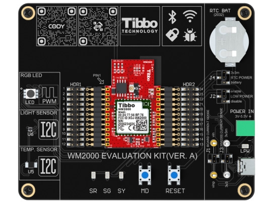
The newly released WM2000EV is an elegant kit for evaluating the capabilities of the WM2000, Tibbo's programmable Wi-Fi/BLE module.

The kit was designed to be completely self-contained and enable the exploration of the module's features without having to wire in any external circuitry. To this end, the board comes equipped with all essential buttons and status LEDs, temperature and light sensors, as well as a PWM-controlled RGB LED. The included CR2032 battery (installed in a holder) can be used to test out the WM2000's low-power "sleep" mode, in which the RTC continues operating and can wake the module up at a preset time.

To aid you in learning about the WM2000's features and capabilities, we have prepared a tutorial featuring a variety of projects.

Your journey begins with testing the IoT/sensor application that comes preloaded on the kit's WM2000. Follow the accompanying step-by-step guide, and in as little as 10 minutes you will have the WM2000 connected to and reporting the measured temperatures and light levels to the Keen service.

The second chapter teaches you how to wirelessly upload a different application into the WM2000. This application showcases controlling the board's RGB LED from a modern, non-reloading web page. In this step, you will also learn about the module's ability to store two applications at once.

Further steps will explain wireless debugging, using CODY (our project code generator), debugging code wirelessly, connecting to Microsoft's Azure cloud service, as well as using the WM2000 in BLE-enabled access control applications.

The kit is powered via an included USB-C cable, which can also be used as a wired debugging interface accessible from our TIDE and WebTIDE software. To facilitate debugging, the board's USB port is connected to the serial debugging pins of the WM2000 via a USB-to-serial converter IC. Wired debugging is useful when wireless debugging via Wi-Fi is unavailable or inconvenient.

Two pin headers are provided for easy access to the WM2000's pins. The module itself is held in place by spring-loaded pins and can be easily popped out and back in. The board even features jumpers and test points for measuring the current consumption of the board and the module.

Order Samples Now!

Ubuntu-based Distribution for the LTPP3(G2) Board

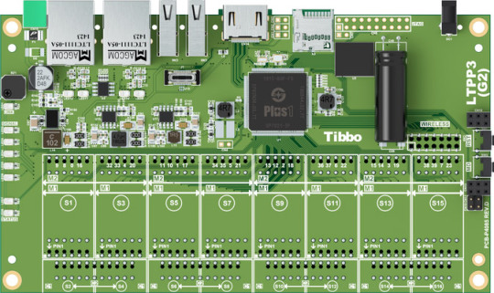
To facilitate the rapid development and deployment of Tibbo Project System (TPS)-based automation and IoT applications while offering our users a familiar environment, we have created an Ubuntu-based Linux distribution.

Ubuntu is one of the world's most popular flavors of Linux. It runs on all kinds of platforms and architectures, and there is a massive amount of community resources available for all project types.

Tibbo's Ubuntu-derived distribution is ideal for system integration, one-off projects, low-volume applications, educational props, and rapid prototyping of products, as well as experimentation and exploration. It provides a user experience similar to that of single-board computers such as Raspberry Pi, but on an extendable hardware foundation that was purpose-built for IoT and automation projects.

Those familiar with Ubuntu will find themselves at home on this new distribution offered by Tibbo. For example, there is a Personal Package Archive (PPA) that is accessible directly through the standard package management utility, apt-get. The PPA contains several tools to help you get started with our Ubuntu-based distribution on the LTPP3(G2) as quickly and effortlessly as possible.

The LTPP3(G2) is a member of the TPS family. A popular choice for automation and IoT projects, our TPS lineup includes the mainboards, I/O modules called Tibbits, and attractive enclosures. The LTPP3(G2) is a Linux mainboard designed around our advanced Plus1 chip.

Included in the PPA, the Out-of-Box Experience (OOBE) script simplifies the device's configuration with a series of interactive prompts that guide you through the process of setting up Wi-Fi/Bluetooth connectivity and the board's Ethernet ports for pass-through or dual-port operation.

Despite its young age, our Ubuntu-based distribution is already hard at work at our manufacturing facility in Taipei. For example, we use LTPP3(G2) boards for testing Tibbits during their production. Employing two high-definition cameras and a touchscreen, this system serves as the testbed for different Tibbits. Thanks to the power of the Plus1's pin multiplexing (PinMux), the individual I/O lines of the board can be remapped on the fly to cater to the needs of whichever Tibbit is being tested at the moment — no kernel rebuild or reboot required. On this new distribution, the board's GPIO lines are reconfigurable in code, much like they are in a typical Tibbo BASIC application.

While this effort remains a work in progress, the development of our Ubuntu-based distribution has reached a point where we feel comfortable sharing a working build with you. We have prepared a repository that contains not only the latest working image, but also automation scripts for customizing your builds through Docker.

We invite you to join us in exploring the exciting opportunities opened up by this new distribution. As always, we welcome your feedback to help us deliver useful solutions tailored to your needs.

Visit the LTPP3(G2) Page!

[idein-inc]

Released Actcast alpha

We have released an IoT platform service named Actcast. It is free of charge alpha release. Please give it a try!

URL of the service: https://actcast.io

What is Actcast?

Actcast is an IoT platform service aiming to handle every information in the physical world by software.

Most of existing IoT systems are using relatively simple data sources such as a temperature-humidity sensor, a vibration sensor, a button switch and so on. On the other hand, with Actcast, you can use perception techniques such as image recognition based on deep learning to obtain diverse information.  

Application fields are from security, in-store marketing, digital signage, visual inspection, inventory management, infrastructure monitoring and so on.

The main features of Actcast are:

Low initial costs

Low running costs

Appropriate treatment of privacy and confidential information

Remote device management and software update

Low Initial Costs

We have been doing R&D for executing deep learning inference on Raspberry Pi series to reduce costs for devices. Watch our achievements in the following video.

Usually, expensive computers are required to run deep learning inference. With our technology, the initial cost for a device becomes less than 100 USD including the camera module. Besides following facts: there are lots of information about Raspberry Pi on the Web, there are many hardware products compatible with such as camera modules, sensor modules, and cases, the supply is stable, and so on, will save cost for initial development, especially in time cost.

We realized the potential of Raspberry Pi as a hardware platform for deep learning inference 3 years ago and have been developing tools such as optimizing compiler specialized for deep learning models. In the development of Actcast, we place importance on acceleration techniques which keeps the model mathematically equivalent. Although, it is a severe condition for speeding up because it does not reduce the amount of computation, it enables automation of deployment of deep learning models to devices without trial and error process to repeat model compressions and accuracy tests for achieving accuracy.

Taking these advantages, we are designing a mechanism and a business model that allows many applications to gather on Actcast. Our goal is to make Actcast a place where a wide variety of applications are available, and every user can construct advance IoT system by just combining appropriate application.

Low Running Costs

In the Actcast’s way, inferences such as image recognition are executed on the edge devices, and only summarized information are sent to the Web. This concept is called Edge Computing.

This architecture significantly reduces the communication cost and server cost compared with that of sending data to the server and analyzing on it. Let’s consider people detection, for example. If inference with 5 fps is necessary, the number of images processed is 13 million per month. Communication and computation occur for all of these images when computation run on a server.

On the other hand, with the Actcast’s way, communication occurs only for the number of people detected by the camera. Also, since the data sent has already been analyzed, the computation cost on the server does not occur.

Appropriate Treatment of Privacy and Confidential Information

Edge Computing also has the advantage of reducing the leakage risk for privacy and confidential information. It's because devices don't have to send unnecessary data to the server. As interest in privacy is growing more and more, we think the concept of Edge Computing becomes essential. 

Remote Device Management and Software Update

You can manage devices registered to Actcast remotely with the following operations:

Alive monitoring

Check the status of the device and software

Install/update/switch/configure software

We think that continuous progress is necessary for the system with machine learning technology. Because it is impossible to create an algorithm with 100% accuracy, it is important to keep using new technologies, collect data and make improvements day by day. In edge computing, the software runs on the device in the field, so the remote update of the software is an essential function.

About alpha version

With this alpha version, you can use applications we prepared in advance to experience the concept of acquiring real-world information and connecting to the web.

You can run demos like the ones on the above with Raspberry Pi on your hand. We are happy if you can report on SNS when it works as expected. Because it is under development, We think there are some problems. Please tell us in the following repository in such cases.

https://github.com/Idein/actcast-support

Toward official release

We are going to develop SDK for enabling users can create custom applications using custom models, make performance improvements, and add some features. Also, we’ll work on making application examples utilizing Actcast. Also, we need to strengthen the structure for service operation.

We think that it can be useful if users can collect data and train models as well in Actcast, so we’ll try to implement Neural Architecture Search and others.

We are looking for talented personnel. We are waiting for your application! https://idein.jp/career

Also, we are looking for partner companies since business development using Actcast requires various elements such as prototyping, production, sales, installation, operation and maintenance of devices, recognition algorithms tailored to the application, analysis, and visualization on the Web, UI, telecommunication, system integration and so on. Companies that become partners have advantages such as early access to SDKs and functions under development. For details, please see the following document.

https://actcast.io/docs/files/partner_program.pdf

[droneseco]

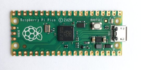
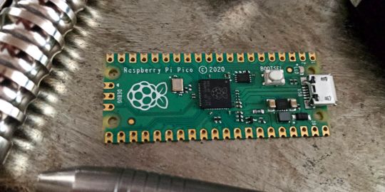
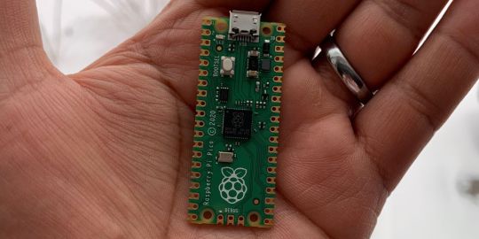
A Peek at the Pico, Raspberry Pi's Newest Petite Powerhouse

Raspberry Pi Pico

8.80 / 10

Read Reviews

Read More Reviews

Read More Reviews

Read More Reviews

Read More Reviews

Read More Reviews

Shop Now

Meet the new Raspberry Pi Pico; a tiny microcontroller filled with big possibilities.

Specifications

Brand: Raspberry Pi

CPU: Dual-core 133Mhz ARM

Memory: 264Kb

Ports: microUSB

Pros

Powerful ARM Processor

Micro-USB Connectivity

Breadboard Mountable

Easy-To-Use Interface

Absolutely Adorable

Inexpensive

Cons

No Wi-Fi or Bluetooth connectivity

No Header Pins

I/O Port Labelling on One Side Only

No USB-C Connectivity

Buy This Product

Raspberry Pi Pico other

Shop

// Bottom var galleryThumbs1 = new Swiper('.gallery-thumbs-1', { spaceBetween: 10, slidesPerView: 10, freeMode: true, watchSlidesVisibility: true, watchSlidesProgress: true, centerInsufficientSlides: true, allowTouchMove: false, preventClicks: false, breakpoints: { 1024: { slidesPerView: 6, } }, }); // Top var galleryTop1 = new Swiper('.gallery-top-1', { spaceBetween: 10, allowTouchMove: false, loop: true, preventClicks: false, breakpoints: { 1024: { allowTouchMove: true, } }, navigation: { nextEl: '.swiper-button-next', prevEl: '.swiper-button-prev', }, thumbs: { swiper: galleryThumbs1 } });

We’ve managed to get our hands on the coveted Raspberry Pi Pico. Today, we’re going to be looking at some of the most important features and putting it toe-to-toe with some of the biggest names in small electronics.

We’ll be showing you what the Pico can do, and we’ll get you started with MicroPython, one of Pico’s supported programming languages. We’ll even offer up some code to try in case you decide to buy a Pico of your own.

What Is a Raspberry Pi Pico?

Raspberry Pi Pico is a new budget microcontroller designed by Raspberry Pi. It’s a tiny computer built around a single chip, with onboard memory, and programmable in/out ports. Historically, microcontrollers are used in a variety of devices from medical implants to power tools. If you have an electronic device sitting in your vicinity, there’s a good chance that there’s a microcontroller inside of it.

Key Features of the Pico

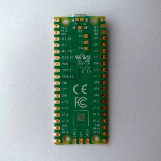
The Pico is built around the RP2040 microcontroller chip, which was designed by Raspberry Pi UK. It’s a Dual-Core ARM processor with a flexible clock that can run up to 133 MHz. The Pico also supports 1.8-5.5 DC input voltage, has a micro-USB input port, and an onboard temperature sensor.

Flanking the chip on all sides are a series of castellations that allow easy soldering to a Veroboard or breadboard. This dual in-line package (DIP) style form factor is stackable, and can also be used in carrier board applications.

Technical Specifications

21 mm x 51 mm

264kb on-chip RAM

2 MB on-board QSPI flash

2 UART

26 GPIO

2 SPI controllers

2 ISC controllers

16 PWM channels

Accelerated integer and floating-point libraries

3-pin ARM Serial Wire Debug (SWD) port

What’s So Special About the Pi Pico?

The Pi Pico is a different kind of microcontroller. It’s Raspberry Pi’s first, and it features ARM technology in its RP2040 silicon chip. Many technology companies are embracing silicon ARM chips, with major manufacturers like Apple leading the charge.

The punchy little Pico packs a staggering 26 multifunction general purpose input/output (GPIO) ports, including 3 that are analog. Alongside these ports are 8 programmable input/output (PIO) ports. Compare this to other microcontrollers like the Arduino Nano, and the Pico packs roughly 18% more GPIO capability.

The most considerable difference between the Pico and its competitors, however, is the $4 price tag. Low cost is the main selling point of this unique offering.

At launch, many online retailers sold out of the device due to the interest and Raspberry Pi’s favorable reputation. By setting the price so low, the Pico opens the door for a new class of high-powered, budget microcontrollers.

There are many potential applications for the new Pico. With its onboard temperature sensor, the device is an obvious choice for IoT projects.

One talented retro gaming enthusiast even used a Pico to build a gaming console with full VGA video support.

This means that makers who have been curious about Raspberry Pi, or microcontrollers in general, now have the ability to experiment for less than the price of a fancy cup of coffee.

Related: The Raspberry Pi Comes of Age With the Pi 400 Desktop

The Raspberry Pi Pico Processor

The RP2040 ARM chip is an interesting choice for the Pico. At 133MHz, the chip is capable of leaving more expensive boards, like the Arduino Uno, in the dust.

Using ARM processors seems to be an emerging trend in the world of microcontrollers. In addition to Raspberry Pi, both Sparkfun and Adafruit also offer boards with similar ARM technology.

The industry-wide switch was made for a single reason—speed. ARM processors give a considerable boost over standard Atmel chips. In a board this size, using an ARM processor is like dropping a fully kitted Porsche engine into a Volkswagen. On the other hand, many microcontrollers don’t require that much processing speed. Yet.

Ramping up performance means that makers who want to push the limits of the Pico will have an abundance of power to do so.

The I/O Ports

The GPIO ports on the Pi Pico feature several interesting functions for common uses such as operating a screen, running lighting, or incorporating servos/relays. Some functions of the GPIO are available on all ports, and some only work for specific uses. GPIO 25, for example, controls the Pico’s onboard LED, and GPIO 23 controls the onboard SMPS Power Save feature.

The Pico also has both VSYS (1.8V — 5.5V) and VBUS (5V when connected to USB) ports, which are designed to deliver current to the RP2040 and its GPIO. This means that powering the Pico can be done with or without the use of the onboard micro-USB.

A full list of the I/O ports is available on Raspberry Pi’s website in its complete Pico documentation.

Pico vs. Arduino vs. Others

One question on the minds of many makers is whether or not the Raspberry Pi Pico is better than Arduino?

That depends. Pound-for-pound, higher-end Arduino boards like the Portenta H7 make the Pico look like a toy. However, the steep cost for a board of that caliber might be a tough pill for the microcontroller hobbyist to swallow. That's why the smaller price tag on the Pico makes it a win for makers who enjoy low-risk experimentation.

Along with minimal cost, the Raspberry Pi jams an extensive feature set into the Pico, comparable to boards like the Teensy LC, and the ESP32. But neither of these competitors manage to challenge the budget-friendly Pico on price.

That's what makes the Pico such a fantastic value, and a great choice for hobbyists and power users alike.

The Pi Pico: What’s Not To Love?

Unfortunately, to drive the price of the Pico down, Raspberry Pi had to make a few compromises. The most notable of which is the lack of an onboard radio module. Neither Bluetooth nor Wi-Fi is supported without add-ons.

The Wi-Fi limitation can be eliminated by adding a module like the ESP-01. Bluetooth support may prove a bit more challenging. If you need an all-in-one solution for your products, you’re better off skipping the Pico, and spending a little extra for something like the Pi Zero W, or ESP32.

Additionally, many early adopters are complaining about the lack of GPIO labeling on the top of the board. Raspberry Pi provides an extensive amount of documentation on its website to address this, but pointing-and-clicking, or thumbing through paperwork when you have a hot soldering iron in your hands isn’t often desirable.

Lastly, the lack of I/O pin headers is something of an issue for some, as it means less convenience when swapping I/O components. This minor annoyance can be solved via the use of leads, soldering the component wiring directly to the Pico, or using a breadboard.

If you’ve been using microcontrollers or small electronics for any period of time, then an unpopulated board is most likely a non-issue. Of course, you could also add your own pin headers if you plan on regular experimentation with different external components.

The final rub with the Pico is the micro-USB port. With many other microcontrollers like the Portenta H7 moving toward USB-C, Raspberry Pi's micro-USB port seems dated.

Logically however, the decision to use micro-USB makes sense. It was done by Raspberry Pi to keep costs as low as possible, and to keep interface capability almost universal. Everyone we know has at least a few micro-USB cables tucked away somewhere in their homes.

However, with future versions, a USB-C interface would be a nice addition to an already spectacular package.

Related: A Beginners Guide To Breadboarding With Raspberry Pi

Programming the Raspberry Pi Pico

Interfacing with the Pi Pico can be done via C/C++, or via MicroPython in the Read-Eval-Print-Loop or REPL (pronounced “Reh-pul”). The REPL is essentially a command line interface that runs line-by-line code in a loop.

In order to access the REPL, you’ll need to install MicroPython onto the Pico. This process is simple and only involves four steps.

Installing MicroPython

Download MicroPython for Raspberry Pi Pico from the Raspberry Pi Website

Connect the Pico to your computer via micro-USB while holding the BOOTSEL button

Wait for the Pico to appear as an external drive

Copy the MicroPython file to the Pi Pico, and it will automatically reboot

You can access the REPL in a number of ways. We used the screen command in a macOS terminal window to access the serial bus connected to the Pico. To accomplish this with Terminal, you’ll first open a new terminal window, then type ls /dev/tty*

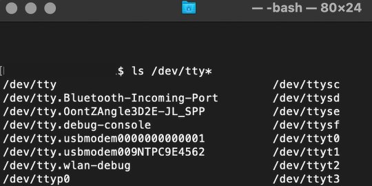
From there, find the port where the Pico is connected. It should be labeled something like /dev/tty.usbmodem0000000000001. Then run the command:

screen /dev/tty.usbmodem0000000000001

Your cursor should change. Hit Return and the cursor will change again to >>>.

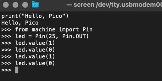
In the image below we've included the classic Hello World (Hello, Pico) command-line program in the REPL, along with a few lines of code that will turn the Pico's LED on and off. Feel free to try them yourself.

For more information, we recommend you invest in the official starter guide to MicroPython that Raspberry Pi has published on their website.

Download: MicroPython for Raspberry Pi Pico (free)

Using the Raspberry Pi Pico With Thonny

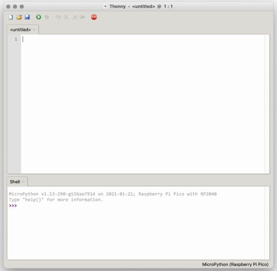
If you’re looking for a more proper coding environment, the Raspberry Pi Pico will also allow access to the REPL with Thonny. To enable this feature, first download and install Thonny. Once installed, connect your Pi Pico. Open Thonny and you'll see information indicating your Pico is connected in the Shell.

At the bottom right of the screen, you should see a version of Python. Click this version and select MicroPython (Raspberry Pi Pico) from the drop-down menu.

Now you can type commands into the Shell, or you can use Thonny’s editor to write or import multiple lines of code.

The abundance of interface possibilities make the Raspberry Pi Pico easy to program. For those who are familiar with MicroPython, this should be nothing new. For beginners, however, Thonny provides a powerful interface and debugger to get started with programming.

Download: Thonny (Free) Windows | Mac

Should I Buy the Raspberry Pi Pico?

The Raspberry Pi Pico is a powerful budget board that is perfect for hobbyists, or makers just starting out with microcontrollers. The documentation, low cost, and wide range of possibilities for the Pico also make it a great choice for seasoned small electronics wizards. If you’re a DIYer who loves to tinker, or you just want to challenge yourself to a weekend project, then you’ll love playing with the Pico.

On the other hand, if you don't have one or more projects in mind that need a microcontroller, then this board is probably not for you. Also, if your project needs Wi-Fi connectivity or Bluetooth, then the Pico won’t scratch that itch. And finally, for users who aren’t comfortable learning MicroPython, or exploring C/C++, the Pico isn't ideal. And remember: this Raspberry Pi is not like the others. It will not run a full Linux operating system.

But, if you dream in Python, or if you love the smell of solder, then you won't regret grabbing this tiny powerhouse. Most of all, if the sight of the sports-car-sleek RP2040 gets your creative gears turning, then we think you’ll really benefit from picking up the Pico.

Serving up Several Sweet Possibilities

While it isn’t perfect, the Raspberry Pi Pico is a strong entry into the world of microcontrollers. The reputation that Raspberry Pi has built for quality electronic components at a relatively low price extends to the Pico.

It’s everything a Raspberry Pi should be: small, sweet, and superb. It’s beautifully designed, and extremely inexpensive. But the best part isn’t the looks or the low cost.

The best part about this small wonder is picking it up, and holding it in your hands. It's feeling the tug of electronic inspiration. It's realizing just how powerful the Pico is, and what it means for microcontrollers going forward.

And truthfully, we think it's amazing that something as small as the Pico can offer so many unique possibilities.

A Peek at the Pico, Raspberry Pi's Newest Petite Powerhouse published first on http://droneseco.tumblr.com/

[itinerancianet]

Raspberry Pi 4 ya tiene caja oficial con refrigeración por ventilador: cuesta apenas 5 dólares

Raspberry Pi 4 ya tiene caja oficial con refrigeración por ventilador: cuesta apenas 5 dólares

Raspberry Pi Foundation ha anunciado una serie de productos interesante este año. La Raspberry Pi 4 como uno de los productos estrella, pero también la Raspberry Pi Compute Module 4 o el interesante Raspberry Pi 400, un teclado con ordenador integrado. Ahora se suma un nuevo producto: un ventilador.

En Xataka

Raspberry Pi 4 Model B, análisis: doble de potencia para un mini PC milagroso,…

[plumpoctopus]

PHYSICS

GENERAL PHYSICS I & II to be accompanied by lab instruction.   Courses of General Physics I & II and Vibrations & Waves can have lab experiments for mechanical, electromagnetic and electromechanical systems involving simulation, coding and microcontrollers. Such includes becoming introduced early to elementary debugging and calibrating schemes. Modelling through sensing (with curve fitting) compared to theoretic modelling, analytical solutions. Simulations for of real systems concern central scheme finite difference, Runge Kutta, etc., etc., etc.  In this “modern era” the ability to competently execute simulation and coding with primitive real systems will be crucial to a student’s future with innovation, relevance, commerce and self-reliance. Such activities builds personal independence and ability with the potential for various projects that’s quite cost effective. Students in such foundational physics courses should be exposed to microcontroller usage at such an early stage, to remain relevant in the future and to build professional relevance with necessary technology. An additional economic incentive is that with such skills developed one opens themselves to engineering paths and “real world ability”; physics ultimately can’t be separated from engineering and programming in the long run. Coding is very important, namely, repetitive copying is not enough; one must really understand what they’re doing in order to really advance in anything. Code lines will be analysed concerning respective purpose. There will be quizzes and the final will involve coding. Questions concern interpretation, filling in lines & patches, truth or false, set up procedures, sensibility of codes with logistics and procedure. The following are just a few experimentation examples of the modernized versions of labs done in course labs. For the other conventional labs one must develop the modernized experiment counterparts. --Comparative schemes for free fall Estimate your local gravitational acceleration with Arduino:        https://www.subsystems.us/arduino-project---gravity.html Interfacing DIY Arduino Photogate Timer:        http://community.wolfram.com/groups/-/m/t/1047262 Medida de g com a placa Arduino em um experimento simples de queda-livre: https://arxiv.org/pdf/1511.08231.pdf Moya, A. A., An Arduino Experiment to Study Free Fall at Schools, Phys. Educ. 53 (2018) 055020 (4pp) --Mass-Spring system Tong-on, A., Saphet, P. and Thepnurat, M. et al, Simple Harmonics Motion Experiment Based on LabVIEW Interface for Arduino, Journal of Physics: Conf. Series 901 (2017) 012114 Will try modules for different masses and springs to observe any possible deviation from the ideal model; different combinations among those three parameters. Varying amplitude, frequency, period and means to model possible air resistance. Pursuit of determining spring constants. --Pendulum Wong, W. et al, Pendulum Experiments with Three modern Electronic Devices and a Modelling tool, J. Comput. Educ. (2015) 2(1):77–92      https://app.ph.qmul.ac.uk/wiki/_media/ajm:teaching:arduino-pi:projects:arduino:simple_pendulum.pdf      https://create.arduino.cc/projecthub/coderscafe/automated-simple-pendulum-7c5bc3 (disregard laser cutter) In some coding design one retrieves information such as the pendulum’s period from voltage applied in respective module. Will try modules for different acute angles (up to 60 degrees), lengths and masses to observe any deviation from the ideal model; different combinations among those three parameters. Varying amplitude, frequency, period and means to model possible air resistance. --Espindola, P. R. et al, Impulse Measurement Using an Arduíno, Phys. Educ. 53 (2018) 035005 (4pp) --An experiment in Moment of Inertia with Raspberry Pi/Arduino https://community.wolfram.com/groups/-/m/t/181641 In this experiment one must determine the right model for objects down an incline plane. Objects of concern are spherical in nature, but some are solid spheres while others are spherical shells. For such objects there two types of kinetic energy, being translational and rotational, where both play important roles in dynamics and trajectories. Proof: consider the conservation problems where a ball starts at some altitude on some incline plane. The results you would get in the experiment exceeds the case of only considering translational kinetic energy. --Goncalves, A. M. B., Cena, C. R. and Bozano, D. F., Driven Damped Harmonic Oscillator Resonance with an Arduino, Phys. Educ. 52 (2017) 043002 (4pp) --Prima, E. C. et al, Heat Transfer Lab Kit using Temperature Sensor based Arduino for Educational Purpose, Engineering Physics International Conference, EPIC 2016, Procedia Engineering 170 (2017) 536 – 540 --Galeriu, C., An Arduino Investigation of Newton's Law of Cooling, Physics Teacher, v56 n9 p618-620 Dec 2018 --Freitas, W. P. S., Arduino-based Experiment Demonstrating Malus’s Law, Phys. Educ. 53 (2018) 035034 (4pp) --Organtini, G. et al, Arduino as a Tool for Physics Experiments, Journal of Physics: Conf. Series 1076 (2018) 012026 Here, one can extend to more advance circuits (up to RLC) --Sanjaya, W. S. et al, Numerical Method and Laboratory Experiment of RC Circuit using Raspberry Pi Microprocessor and Python Interface, Journal of Physics: Conf. Series 1090 (2018) 012015 Here, one can extend to more advance circuits (up to RLC). As well, one isn’t to be subjugated to populism with Python. --Bezerra et al, Using an Arduino to demonstrate Faraday’s Law, Phys. Educ. 54 (2019) 043011 (6pp) --Huang, B., Open-source Hardware – Microcontrollers and Physics Education - Integrating DIY Sensors and Data Acquisition with Arduino, 122nd ASEE Annual Conference & Exposition June 14 -17, 2015  Seattle, Washington --Arduino in the Physics Lab      https://ec.europa.eu/programmes/proxy/alfresco-webscripts/api/node/content/workspace/SpacesStore/59719c38-c26e-4a8d-b853-ce56e04be930/MoM_PRESENT_Monday_Arduino%20in%20the%20Physics%20Lab_C_A.pdf Here, one can extend to more advance circuits (up to RLC) --For labs involving conservation of energy (translation and rotational influence) one can apply toy ramps and rolling rings, discs, hollow balls and solid balls. One can observe whether neglecting rotational kinetic energy can be catastrophic concerning destination of rolling. Conservation of momentum can be incorporated into labs as well. --Conservation of angular momentum Part A Conservation of Angular Momentum Example – YouTube      https://www.youtube.com/watch?v=DtxxmTdQ2Jc In such an experiment would like to extend experiment to fit two torque sensors and two angular momentum sensors without considerably distorting the mass distribution of the rotating bodies. One would like to acquire time continuous data for both measures. Angular momentum to be expressed in terms of angular velocity. All masses applied should be known. Motor operation measures should be known for time T when initiating experiment and what not. How can one verify conservation of angular momentum? How are the torques related to conservation of angular momentum? Co-rotation and counter rotation ability would be nice. Trials in lab may be warranted. Part B One would like to then construct an apparatus where a portion of its mass can contract or extend during the apparatus’ rotation. A torque sensor and a angular momentum sensor without considerably distorting the mass distribution of the rotating bodies. One would like to acquire time continuous data for both measures. Angular momentum to be expressed in terms of angular velocity.  All masses applied should be known. Motor operation measures should be known for time T when initiating experiment and what not. How can one verify conservation of angular momentum? How is torques related to conservation of angular momentum? Co-rotation and counter rotation ability would be nice. Trials in lab may be warranted. Physics technology for the biological sciences, social sciences, business, computational finance and actuarial studies: PHYPHOX https://phyphox.org  and  https://www.youtube.com/watch?v=sGAZQNUBYCc Such can be directed to students in career pursuits outside of engineering and the physical sciences. Technology resources for the physical sciences and engineering shouldn’t be exhausted or marginalized by those in other fields. Curriculum:   --Core Courses Scientific Writing I & II, General Chemistry I & II, General Physics I & II, Vibrations & Waves, Fluid Mechanics, Advanced Mechanics I, Electromagnetic Theory I, Modern Physics, Methods of Mathematical Physics, Quantum Physics I & II --Mandatory Courses     Found in Computer Science post            Data Programming with Mathematica     Found in Computational Finance post           Calculus for Science & Engineering I-III           Ordinary Differential Equations           Numerical Analysis           Partial Differential Equations           Probability & Statistics           Mathematical Statistics NOTE: after Calculus III and General Physics II things become hectic, so plan well.  Specialization tracks to pursue (being mandatory options tracks): 1. Advanced Mechanics II; Electromagnetic Theory II; Introduction to Astronomy; Stochastic Models & Computation (COMP FIN); Machine Learning for Physics & Astronomy 2. Chemical Physics I & II (check CHEM); Introduction to Astronomy; Stochastic Models & Computation (COMP FIN); Machine Learning for Physics & Astronomy 3. Intro to Astronomy; Techniques in Observational Astronomy I & II; Space Science I & II; Machine Learning for Physics & Astronomy 4. Intro to Astronomy; Techniques in Observational Astronomy I & II; Space Science I & II; Particle Physics I 5. Introduction to Astronomy; Space Science I & II; Tensor Analysis & Riemannian Geometry; Computational General Relativity 6. Intro to Astronomy; Techniques in Observational Astronomy I & II; Tensor Analysis & Riemannian Geometry; Computational General Relativity 7. Introduction to Astronomy; Techniques in Observational Astronomy I & II; Particle Physics I & II 8. Introduction to Astronomy; Space Science I & II; Particle Physics I & II 9. Introduction to Astronomy; Introduction to Optics; Advanced Optics Lab; Particle Physics I & II 10. Chemical Physics I & II (check CHEM); Stochastic Models & Computation (COMP FIN); Statistical Physics I & II 11. Intro to Astronomy; Techniques in Observational Astronomy I; Stochastic Models & Computation (COMP FIN); Statistical Physics I & II   Physics electives options --> Introduction to Optics Advanced Optics Lab Introduction to Astronomy Techniques in Observational Astronomy I & II Machine Learning for Physics & Astronomy Space Science I & II Tensor Analysis & Riemannian Geometry Computational General Relativity Statistical Physics I & II Particle Physics I & II NOTE: students can make a mandatory specialization track with departmental guidance with courses outside of physics -- Chemistry electives options --> Organic Chemistry I Analytical Chemistry Inorganic Chemistry I & II Chemical Physics I & II Molecular Modelling       Special permission from both Chemistry department chair and course instructor towards proper and official enrolment

Mathematics electives options --> Stochastic Models & Computation R Analysis (requires special permission from instructor and chairperson) Data Science Sequence (requires special permission from instructor and chairperson)   Oceanography/Meteorology electives options --> Physical Oceanography Physical Oceanography Techniques Fundamentals of Atmosphere & Ocean Dynamics for Oceanography Coastal & Oceanographic Numerical Simulation Techniques Data Analysis in Atmospheric and Oceanic Sciences. NOTE: for course electives outside of physics there are others posts with their detailed descriptions. NOTE: General Physics I & II are to be considered elementary requirements in the physical sciences and geophysics. If you want to be a perfectionist in General Physics I & II, practice those problems OVER AND OVER INDEPENDENTLY...AND PERSONALLY BUY THE SUPPLEMENTAL MANUAL; problems are never going to change in nature. Anything else, being a bunch of impractical junk collector’s contraptions to whosoever’s interest. Else, there’s Systems Modelling I & II  you can take out of engineering as electives, but will have no influence on the Physics programme. Description of some courses--> General Physics I (with labs): This is the beginner level course as an introduction to physics. Students must have Calculus I as prerequisite. Calculus will be used in course to exhibit its foundational role in physics. Texts:    Fundamentals of Physics, by Halliday, Resnick and Walker    Physics for Scientists & Engineers, by Serway and Jewett Tools:   Engineering calculator   Stationery   Graphing paper   Standard measuring stationery Grading    Homework: 10%    6 Quizzes (best 5 out of 6): 15%    3 Midterm Examinations (best 2 out of 3): 30%    Final Examination: 25%    Labs 20% Quizzes --> Don’t be careless with performance on quizzes, say, the accumulation is often taken for granted. Homework --> Homework will come from texts AND others sources Quizzes --> Quizzes will be based on lectures and homework Labs Students are expected to print out their lab documents to be prepared for lab. Labs will also have quizzes. Labs will be what was described in the beginning. Exams --> Exams will be based on homework and quizzes   Lecture Topics -->   Vectors   Rectilinear motion   Motion in 2 or 3 dimensions   Projectile Motion   Newton’s Laws of motion   Applying Newton’s Laws   Free-body diagrams & applications   Work & Kinetic Energy   Circular Motion & Centripetal Force   Potential Energy & Energy Conservation   Momentum Impulse and Collisions   Rotation of rigid bodies   Dynamics of Rotational Motion   Periodic Motion   Mechanical waves   Sound and Hearing   Fluid Mechanics   Gravitation (well treated) Prerequisite: Calculus I General Physics II (with labs): The objectives of this course are:   (1) To develop a basic understanding of the laws of electromagnetism.   (2) To develop the ability to apply these new concepts to physical situations.   (3) To develop an appreciation for the role that electromagnetism plays both in our modern society and in the universe. Texts:     Fundamentals of Physics, by Halliday, Resnick and Walker     Physics for Scientists & Engineers, by Serway and Jewett Tools:    Engineering calculator    Stationery    Graphing paper    Standard measuring stationery Grading     Homework: 10%     6 Quizzes (best 5 out of 6): 15%     3 Midterm Examinations (best 2 out of 3): 30%     Final Examination: 25%     Labs 20% Quizzes --> Don’t be careless with performance on quizzes, say, the accumulation is often taken for granted. Homework --> Homework will come from texts AND others sources Quizzes --> Quizzes will be based on lectures and homework Labs Students are expected to print out their lab documents to be prepared for lab. Labs will also have quizzes. Labs will be what was described in the beginning. Exams --> Exams will be based on homework and quizzes Lecture Topics -->   Electric Charges & Electric Forces   The Electric Field   Gauss’ Law   Electric Potential   Potential & Field   Current & Resistance   Fundamentals of Circuits   The Magnetic Field   Electromagnetic Induction   Electromagnetic Fields & Waves   AC Circuits   Interference & Light Prerequisites: General Physics I, Calculus II   Vibrations & Waves: Grading:     25%: Assignments (set weekly)     25%: Mid-term     25%: Labs     25%: Final exam Typical Texts:     Georgi, Howard. (1992). The Physics of Waves. Benjamin Cummings     Vibrations and Waves, by A. P. French LABORATORY COMPONENT --> Laboratory skills are highly practical and give you an appreciation for difficulty of working both precisely and accurately. This requires discipline and patience, that can take time to develop. 1. Physics of sound -How is all such manipulated to achieve acoustic goals?     Physics of blunt mechanics (striking, plucking, blowing, etc., etc.) to generate sound. Physics at the microscopic level for sound generation. -Modelling the transfer of sound waves -Speed of sound      Modelling the speed of sound w.r.t. media.      Modelling for variability with pressure, density, elasticity, temperature      Measuring the speed of sound with a single-board microcontroller and ultrasonic sensor; confirm experiment results with prior modelling.     May try to experimentally verify as well for variability with pressure, density, elasticity, temperature 2. To avoid massive expense for laboratory with particular contraptions and “classical equipment” some of the lab activities will highly resemble microcontroller applied experiments described at the beginning of this post.           Mechanical systems (various)                Review physics and modelling           Electric Circuits (various)                Review physics and modelling 3. Fluid Damped Harmonics -First, will review modelling and consequences -https://www.thepocketlab.com/educators/lesson/damped-simple-harmonic-motion 4. Chladni Plates -Physics and modelling must be developed. -Understanding the role of nodes and anti-nodes. -Can Chladni Plates be simulated? -Will also be building multiple Chladni Plates to observe and record behavior. With respect to the properties and geometry of the membrane will try to analytically develop a model to map the nodes and anti-nodels. Can such be simulated? -How to map nodes and anti-nodes on instruments? -We want data. Data for frequencies and (Eigen)modes will be of interest towards models. 5. Will also pursue vibrations where particles come together to form microspheres “fluids”. What conditions are the cause for such “fluid” behaviour? 6. Acoustic levitators -Physics and mathematical modelling must be developed -Understanding the role of nodes and anti-nodes. Gor’kov potential, accoustic radiation force, and elastic constant as a second order derivative. Modelling the complex acoustic pressure. Assisting Literature:      Jackson, D. P. and Chang, M. (2021). Acoustic Levitation and Acoustic Radiation Force. American Journal of Physics, volume 89, Issue 4, 383      Andrade, M. A. B., Pérez, N. & Adamowski, J. C. (2018). Review of Progress in Acoustic Levitation. Braz J Phys 48, 190–213      Andrade, M. A. B., Marzo, A. & Adamowski, J. C. (2020). Acoustic Levitation in Mid-Air: Recent Advances, Challenges , and Future Perspectives. Applied Physics Letters, Volume 116 Issue 25 -Developing the model, pressure field code and simulation -An example of what must be pursued:     Acoustic Levitator DIY – TinyLev-Levitate Liquids & Insects at home – YouTube Basic components:     Ultrasonic transducers     Aluminium reflector     Driver board     Arduino board (or whatever substitute)     Oscilloscope     Infrared imaging applicable Data from experimentation will be gathered to reconcile with the physics and mathematical modelling.   7. Vibration analysis of an electric motor Wang, C.& Lai, J. (1999). Vibration Analysis of an Electric Motor. Journal of Sound and Vibration. 224. 733-756. Will pursue lab investigation based on such article, etc., etc. 8. Fault detection -Fault detection of electric motors based on vibration analysis -Yamamoto, G. K., da Costa, C. and da Silva Sousa, J. S. (2016). A Smart Experimental Setup for Vibration Measurement and Imbalance Fault Detection in Rotating Machinery, Case Studies in Mechanical Systems and Signal Processing, Volume 4, Pages 8-18 9. Sound from electrical instruments (time permitting) -Modulators, electric keyboards and synthesizers        Modelling the process        May pursue development of scaled down versions, namely, based on single board computers to demonstrate COURSE OUTLINE --> 1. Introductory concepts Periodic motion, superposition of periodic motion. Free vibrations of physical systems. 2. Damped Systems Under/over and critically damped systems. “Q” parameter. 3. Forced Vibrations and Resonance Variation in amplitude with driving frequency. Resonances in damped and undamped systems. 4. Coupled Oscillators Coupled pair of oscillators. Modes of oscillation. Application to N coupled oscillators. 5. Continuous Systems Vibrations on a string. Driven continuous systems. Note: all continuous systems considered will be finite in length   6. Waves and Optics Energy in a wave, boundaries and interference. Huygens-Fresnel principle. Double-slit experiment 7. Nonlinear Vibrations        Wagg D. & Neild S. (2010). Nonlinear Vibration with Control. Solid Mechanics and Its Applications, vol 170. Springer, Dordrecht        Juan Carlos Jauregui, J. C. (2014). Parameter Identification and Monitoring of Mechanical Systems Under Nonlinear Vibration, Woodhead Publishing Prerequisites: Calculus III, General Physics I & II, ODE Advance Mechanics I This course covers Lagrangian and Hamiltonian mechanics, systems with constraints, rigid body dynamics, vibrations, central forces, Hamilton-Jacobi theory, action-angle variables, etc. Course will make use of 14 – 15 weeks. Textbook: TBA Two functions in Mathematica that may be useful (but only for reference)    EulerEquations    VariationalD Basic Expectations -->    Modelling with Newton’s Second Law    Identify generalized coordinates and system representation    Ignorable coordinates & system representation    Lagranigan (Hamiltonian) determination of various systems    Finding Ignorable coordinates to recognise conserved quantities    Resulting explicit set of equations from Euler-Lagrange equations    Solutions of found explicit equations prior    Comparing E-L solutions to solutions of Newton’s 2nd second law        Systems must be treated by both E-L and Newton’s second law    Hamiltonian determination of various systems    Hamiltonian Systems    Comparing Hamilton treatment to solutions of Newton’s 2nd second law       Systems must be comparatively treated by both E-L and Newton’s second law NOTICE FOR BASIC EXPECTATIONS:           -Some mentioned subjects prior will arise on multiple occasions, or will simply resonate throughout.          -I will be a stickler with past intelligence and skills as one advances in course. Hence, for more advance obligations as one progresses will treat prior expectations as primitives to be included, to be well developed and detailed. Homework --> Constituted by typical problem sets Quizzes --> Will reflect homework. There will be 3-5 quizzes. Exams --> There will be 3 exams that will reflect lectures, homework and quizzes. Grading:      Homework 15%      Quizzes 25%      3 Exams 60%     Course Outline -->           Block 1 (will be rapid)-- Translational Kinematics Rotational Kinematics Newton's Laws of motion Free-body diagrams    Mechanics of general bodies (translational, rotational, combination)            Special studies (tension, pulleys, ring, disks, ball, solid sphere, gears) in  planes, inclines, contact surfaces, etc. Second order differential equations model development for systems (subjugated by Newton’s laws of motion modules and free-body diagrams module). Block 2 (will be rapid)-- Conservation laws: Energy, Linear momentum and angular momentum Applications: ballistics (neglecting air resistance), harmonic oscillator (various systems. Frictionless ramps/terrain with relative extrema, etc., etc. involving rings, disks and spheres (hollow and solid). Will also have the alternative approach of acquiring models for systems by making use of energy, linear momentum, angular momentum (some systems will require use of all three physical measures); compare this method to Newton second law approach for all problems. Block 3 -- Generalized coordinates & representation of systems Constraints D'Alembert's principle. Informal exposure to the role of Euler-Lagrange equations and ideal examples Examples of constrained systems Block 4 -- Principle of Least Action (PLA) and its development. Explicit examples. Acquiring the Euler-Lagrange equations from the (PLA). Explicit examples. Euler-Lagrange equations applications Block 5 -- More Lagrangian Mechanics: Unconstrained and constrained Dynamics of excavators and cranes.       Will likely need a CAS AFTER analytical development of models. I don’t care about any pig pen matrix algebra finesse because we don’t have no time for it; no true professional has time for rent seeking ideology. Block 6 -- Hamiltonian Mechanics Block 7 -- Oscillations: normal modes, Kapitza pendulum, Foucault pendulum, Parametric resonance Block 8 -- More Hamiltonian Mechanics, Action. Liouville’s theorem. The Hamilton-Jacobi equation, Action-angle variables, Adiabatic invariants Prerequisites: General Physics I & II, ODE, Calculus III. There is no requirement of Methods of Mathematical Physics as a prerequisite course.   Advance Mechanics II Second course in the Advanced Mechanics sequence. Course focus is to further establish theory in classical mechanics. Course is not a runaway mathematical trainwreck. We have meaningful developments, say, what you’ve analysed or learnt should generally be applicable in the real world, else, you really don’t understand much, and for some reason like "diving off a boat holding a 50 pound cannon ball”. We’re dealing with classical mechanics here, not untested String Theory. Assessment -->     Homework (prerequisite tasks and course level tasks)     3-5 Quizzes (will reflect homework)     3 Exams (will reflect quizzes and homework) Outline--- --Fast review of applied Lagrangian formalism  1. Common coordinates and generalised coordinates; ignorable coordinates; generalized forces and momenta            General notations must be accompanied with various explicit dynamical systems; a means to deter incompetence with real dynamical systems, without reservation.  2. Advance review of the least action principle    3. Ideal systems         Systems without constraints           Summary of coupled oscillations and normal modes using Lagrangian; reconstructing the motion of the system from the normal modes.  4. Central force problems   Obtain the equation of motion in terms of an effective potential and solve for standard central force problems. Lagrangian and Hamiltonian treatment:         Orbit equation         Precession         Deriving a scattering cross-section for a given central force problem  5. Conservation laws, cyclic coordinates symmetries and Noether’s theorem  6. Miscellaneous problems (Newtonian versus Lagrangian) Coriolis effect; rotating top about a fixed point on a flat plane in the presence of gravity; Coriolis gyroscope; Gimbal gyroscope; Rayleigh dissipation function. Townsend, N.C., Shenoi, R.A. Modelling and Analysis of a Single Gimbal Gyroscopic Energy Harvester. Nonlinear Dyn 72, 285–300 (2013) --Role of Lagrange multipliers in constrained systems and solving --Holonomic and non-holonomic constraints  1. Determining the nature of the constraints (holonomic or non-holonomic, time-dependent or static) and forces (conservative or non-conservative) for a given problem, and thereby identify the number of degrees of freedom and select appropriate generalized coordinates.  2. Integrability and Non-Integrability of Holonomic and Nonholonomic systems Flannery, M., R., The Enigma of Nonholonomic Constraints, Am. J. Phys. 73 (3), March 2005.  3. Pendulum examples involving constraints (with or without friction) --Various Nonholonomic constraints applications  1. Swaczyna, M., Several examples of Nonholonomic Mechanical Systems, Communications in Mathematics 19 (2011) 27–56  2. Rolling disc on a horizontal plane (compare with 2 in prior module)  3. Homogeneous sphere rolling without sliding on a horizontal plane rotating with non-constant angular velocity about a vertical axis. Apart from constant gravitational force, no other external forces to act on the sphere.    4. The Bicycle  5. Del Rosso, V., et al, Self-Balancing Two-Wheel Drive Electric Motorcycle Modelling and Control: Preliminary Results, 2018 5th International Conference on Control, Decision and Information Technologies (CoDIT’18), IEEE 2018.   6. Control of Space Vehicles with Fuel Slosh Dynamics   7. Control of a manipulator with a Jerk Constraint   8. PPR robot and 3-PPR planar robot   9. Jin Jung, M., Hwan Kim, J., Development of the Fault-Tolerant Omnidirectional Wheeled Mobile Robot Using Nonholonomic Constraints, The International Journal of Robotics Research Vol. 21, No. 5-6, May-June 2002, pp. 527-539   --Hamiltonian theory  1. Recognise the concepts of Hamilton’s principle and phase-space  2. Hamiltonian and conservation; conserved quantities from cyclic coordinates perspective; recognising the resulting equations of motion  3. Solve Hamilton’s equations of motion for standard problems.  4. Valle, G., Campos, I., and Jim, Jimenez, J., L., A Hamilton-Jacobi Approach to the Rocket Problem, Eur. J. Phys. 17 (1996) 253–257   --Canonical transformations  1. Finding canonical transformations for simple problems to make the problem easy to solve (cyclic coordinates).  2. Testing for the canonical condition using generating functions, the symplectic condition, and Poisson brackets.  3. Applying Poisson bracket formalism to identify constants of motions. Determining time evolution of a generic dynamic variable of interest for a given Hamiltonian using Poisson bracket formalism. --Hamilton-Jacobi Theory (HJ)  1.The prime directive for development concerns only how and when we want to use it with applications; neither how mathematically contorted nor honouring mathematical "magic mushrooms spam”.  2. Applications: mechanics, gravitational, electromagnetic fields            Will also emphasize separation of variables w.r.t to coordinates  3. Numerical Methods  4. Verify that for system in question Lagrangian, Hamiltonian and HJ are consistent with each other --Perpetual Motion and the Laws of Thermodynamics Will have cases studies of attempted devices. Namely, description and modelling, and challenges based on laws of thermodynamics.  Prerequisite: Advance Mechanics I   Fluid Mechanics To develop a fundamental understanding of the science and engineering of fluid mechanics, through rigorous theoretical discussions, analytical examples, practical applications, and computational projects. Fluid properties, hydrostatics, conservation equations, analytic description of simple flows, flow measurement, empirical description of engineering flows, similitude, lift, drag, boundary layers, compressible flows, some engineering applications. Students must have familiarity with conservation principles, vector calculus, and differential equations. Computationally, proficiency in a high-level programming environment (e.g. C/C++, Mathematica, OpenFOAM) to design algorithms and perform calculations, and compared to solutions given by Mathematica. Course will also engage software such as OpenFOAM. Prototypical textbook -->       Munson, et al., Fundamentals of Fluid Mechanics Lab textbooks -->          Ferziger, J. H., Peric, M. and Street, R. L. (2020). Computational Methods for Fluid Dynamics. Springer International Publishing ·        F. Moukalled, L. Mangani and M. Darwish (2015). The Finite Volume Method in Computational Fluid Dynamics: An Advanced Introduction with OpenFOAM and Matlab, Springer Tools -->       Mathematica, OpenFOAM Labs --> Labs will follow determined lecture sets. Will characterise the fluid behaviours of concern, accompanied by characterisation of the differential equations that govern. Analytical solution methods will be mostly overview. Students will initially pursue solutions in Mathematica, identifying the chosen method applied by Mathematica concerning NDSolve; followed by assigned numerical methods building in Mathematica. Will incorporate development with OpenFOAM; manual development of numerical methods in Mathematica will accompany alongside results from Mathematica selection methods and OpenFOAM development. Labs concern modules 5, 7 and 8 treating all topics in respective module.  Exams -->      -Exams will be based on homework      -Exams will incorporate Mathematica activities      -Exams will incorporate OpenFoam activities when appropriate to compare with your acquired Mathematica usage and development. You are permitted 2-3 sheets of loose leaf notes ONLY FOR Mathematica and OpenFoam use.  Computational Fluid Dynamics Project --> Independent projects based on all prior OpenFoam skills development. Assessment -->      Homework      Labs      4 Exams          Computational Fluid Dynamics Project Topics outline --> 1.Fluid Statics -- Pressure variation in a fluid at rest -- Hydrostatic forces on plane and curved surfaces -- Buoyancy and flotation principles 2.Bernoulli Equation -- Derivation of streamline and normal components of the momentum equation -- Static, dynamic and total pressures -- Restrictions on the use of the Bernoulli equation 3.Fluid Kinematics -- Eulerian and Lagrangian descriptions -- Velocity and acceleration field -- Control volume and system representation -- Reynolds transport theorem 4.Integral control volume analysis -- Conservation of mass, momentum and energy for incompressible flow 5.Differential analysis of fluid flow Module will apply Mathematica and OpenFOAM -- Velocity and acceleration field -- Conservation of mass and momentum -- Euler’s inviscid equations of motion -- Potential Flow -- Navier ­Stokes Equations 6.Dimensional Analysis -- Buckingham Pi Theorem -- Modelling and similitude 7.Viscous Flow in Pipes Module will apply Mathematica and OpenFOAM -- Laminar and turbulent flow -- Entrance region and fully developed flow 8. External Flow Module will apply Mathematica and OpenFOAM -- Lift and drag concepts -- Boundary layer concepts 9. Computational Fluid Dynamics Project Prerequisites: Calculus III, Numerical Analysis, and General Physics I. Methods of Mathematical Physics   This course isn’t concerned with being a perfectionist, nor towards retarding attempts to unfairly treat or critique others by claiming teaching education based on something trivial one has practiced a thousand times with nothing better to do. Affinity or innate ability makes the world turn, not a parasitic mathematical fanatic; you can’t compare a mathematician to an engineer or physicist or chemist. Any directive of this course doesn’t primarily concern repulsive trivial manual matrix algebra prowess; people have better things to do than trying to intimidate others with boxes of numbers abiding by linear models. All modules mentioned and detailed subjects will be completed with quality instruction. Course will have integrity in a firm foundation of physics. A major directive of this course is to introduce practical and relevant mathematical tools in a pleasant manner towards the physical sciences and geophysics. It’s really constructive that students consume and digest the material through such fluid and tangible course layout given, rather than them questioning their decision making in career goals, and them not questioning the instructor’s true worth in society. One wants to model physics, rather than attempts of mathematical superiority towards nothing. Mathematical theory will neither drown course nor weaken the focus of the course. Course will be treated in a manner that emphasizes practicality, being a solid foundation for the physical sciences and geophysics, rather than mathematical frolic and parasitic mathematical obnoxiousness.            Homework 20%      4 exams (for ease of mind and for constructiveness) 80% Course Outline -->   --Geometrical Vector Spaces   This module will only concern objects physically meaningful to the physical sciences; notion of dimension will be physical and nothing more. To be relevant to physics one must have a background in physics and understand the physics. Topics in module will be described, developed and categorized towards constructive practical usage in applications. Matrices done manually will be no larger than column size or row size of 3 and will be limited; larger sizes concern computational tool.  1. Structure for Euclidean space         Definitions of field         Vector space         Inner product         Norm         Normed vector space         Metric    2. Linear independence and bases vectors with relation to coordinate systems and transformations. Note: I don’t care about about a bunch of given weirdo matrices out of no where. I only care about coordinate systems and transformations.  3. Gram-Schmidt Process (vectors) and its relevance to basis vectors. Modified Gram-Schmidt (vectors)  4. Transformations between Cartesian coordinate systems: shifts, Euler angle rotations and relation to spherical coordinates or cylindrical coordinates.  5. Transforming differentials and vectors among Cartesian, polar, cylindrical and spherical coordinates.    6. For a respective system identify the basis. Change of basis between prior mentioned coordinate systems. Confirm that magnitude and direction remains unchanged. How does one know that orientation is preserved?  7. Eigenvectors and Eigenvalues of geometric transformations (Mathematica usage to complement). Don’t evangelise the boxes of gibberish finesse, rather, why is it so special that it’s not wasting time --Properties of vectors spaces in Euclidean space with application to coordinates   1. Observing the orientations of vectors and covariant vectors at point p. Mapping for contravariant and covariant vectors, and respective transformation matrices (and will apply actual coordinates).   2. Covariant bases and contravariant bases and observing the orientations at point p (will also apply coordinate systems and transformations).   3. Kronecker delta; dual relationship between contravariant and covariant (basis) vectors   4. Defining the norm via contravariant-covariant “contraction” and its invariance w.r.t to coordinate transformations.   5. Euclidean Metric         i. Properties of distance (or the norm) validated in Euclidean space, namely positive definiteness, non-degeneracy, symmetry and triangular inequality.         ii. Transformation of metric components         iii. Transformation of metric components w.r.t to actual coordinate transformations, and preservation of distance         iv. Use of the Euclidean metric to relate contravariant and covariant components --Common Tensorial Operators Note: higher order tensors will be confined to rank 2.   1. Introducing the concept and structure of the tensor product, it’s geometrical view, and it’s transformation (from “egg shell” form to explicit cases with coordinate systems). Explicit change of coordinates for tensor products among the basis vectors. For a given coordinate transformation how will chosen basis vectors transform. Can you account for all transformed basis vectors? NOTE: will not indulge much on rotation matrices and coordinate, because there are more interesting representations of geometrical objects. Among various coordinate systems will investigate explicitly how tensor components (unique to the tensor product) adjust to preserve equivalence in the manifold.   2. The metric tensor. Will identify its properties and formally recognise tensorial structure, and employing (1) prior towards its properties.       3. Review of gradient (with properties) and the displacement gradient; change of coordinates and verifying equivalency among coordinate systems.   4. Review of directional derivative and properties; change of coordinates and verifying equivalency among coordinate systems.       5. Review of divergence and properties; change of coordinates and verifying equivalency among coordinate systems.   6. Gradient of a tensor field; change of coordinates and verifying equivalency among coordinate systems.         7. Directional derivative of a tensor field; change of coordinates and verifying equivalency among coordinate systems.   8. Divergence of a tensor field; change of coordinates and verifying equivalency among coordinate systems.   9. Review of divergence theorem; change of coordinates and verifying equivalency among coordinate systems.   10. Gauss’ Divergence theorem of a tensor field; change of coordinates and verifying equivalency among coordinate systems.   11. Applications of the Levi-Civita symbol         i. Definition and properties         ii. Determinants         iii. Vector cross product, curl & irrotational fields         iv. Curl of tensor fields; change of coordinates & verifying equivalency among coordinates         v. Review of Green’s theorem and Stokes theorem. Tensorial forms of Green’s Theorem and stokes theorem; change of coordinates & verifying equivalency among coordinates.    12. Will identify non-relativistic tensors in the physical sciences and apply various explicit coordinate transformations as practice, verifying equivalency among coordinates.    13. Electromagnetism             Review of Maxwell Equations             Maxwell Equations in terms of electromagnetic potentials             Lorentz force from Faraday’s Law             Verifying prior holds under coordinate transformations             Is gauge invariance unique to coordinate transformations?             Is gauge invariance preserved under coordinate transformations?             Differentiation between Lorentz transformations and coordinate transformations             Investigate the Lorentz transformations                    Subject to gauge invariance, that’s subject to coordinate transformations             Covariant formulation (with incorporation of all prior developments)             Derivation of  Lorentz force law                             Field, J. H. Derivation of the Lorentz Force Law and the Magnetic Field Concept using an Invariant Formulation of the Lorentz Transformation. CERN: https://cds.cern.ch/record/630753/files/0307133.pdf             Electromagnetic Field Tensor                Will verify preservation under various coordinate transformations                Lorentz transformations under coordinate transformations, say, if is not interested in “Cartesian-like representation”, rather wanting (t, x, y, z) in terms of cylindrical coordinates or spherical coordinates or other, and vice versa.               Model for charged particles with the electromagnetic field tensor --Basic Lagrangian Modelling in Classical Physics For this module, purpose and logistics are emphasized. Namely, comprehending what you’re trying to accomplish, what one needs to formulate, and finishing. For all mechanical systems encountered, reconciliation with Newton’s second law must be established; includes solutions through Newton’s law to compare with E-L approach solutions.  1. Variational principle: curve, surface and general pat for which a given function has a stationary value with existence of extremum. Arriving at the Euler-Lagrange equation.  2. For two-dimensional Euclidean space proving that the shortest distance between two fixed points is a straight line            Conventional calculus (CC)            via Euler-Lagrange equation (E)            For both CC and EL, change of variables (coordinates) amongst Cartesian, cylindrical, and spherical coordinates and establishing equivalence.            Geodesics on the sphere analogy to priors  3. Going from spatial geometries to physics. How does one connect Lagrangian formalism to physics? Was the Lagrangian a meaningful physics concept before being a mathematical “vanity”?  4. Case studies of consideration          Reformulating Newton’s equations of mechanics. Change of variables (coordinates) amongst Cartesian, cylindrical, and spherical coordinates and establishing equivalence. Validating equivalence between Newtonian mechanics and Lagrangian modelling for various classical mechanics problems.          Finding the curve that will allow a particle to fall (by gravity as inverse square model) under the action in minimal time. Then extending to incorporate atmospheric resistance, what will be then?            Finding the Lagrangian density of a vibrating string fixed at both ends, then applying the Euler-Lagrange equations, yielding the wave equation.          Determining the Lagrangian for electromagnetic interaction. Does the resulting E-L equation translate to the Lorentz force? If not, then what?  5. Advance guides -->                   Ferrario, C. and Passerini, A. Transformation Properties of the Lagrange Function. Rev. Bras. Ensino Fís. [online]. 2008, vol.30, n.3 [cited  2020-02-28], pp.3306.1-3306.8                     Sudarshan, E. C. G. and Mukunda, N. (2015). Chapter 5 Invariance Properties of the Lagrangian and Hamiltonian Descriptions, Poisson and Lagrange Brackets, and Canonical Transformations. Pages 31 -44. In: Classical Dynamics a Modern Perspective. World Scientific.  6. Hamiltonian analogy to Lagrangian Modelling Will also include why there’s preference at times for the Hamiltonian over Lagrangian modelling. Basic practical applications. Prior literature excerpt to also apply  7. Hamilton-Jacobi (HJ)          The prime directive for development concerns only how and when we want to use it with applications; neither how mathematically contorted nor honouring mathematical "magic mushrooms spam”.          Applications: mechanics, gravitational, electromagnetic fields               Will also emphasize separation of variables w.r.t to coordinates           Numerical Methods          Verify that for system in question Lagrangian, Hamiltonian and HJ are consistent with each other  8. Investigating Mathematica functions --Orthogonalization of Functions   1. Why do we care about this in physics?   2. Proof of economical practicality in use   3. Seaborn, J. B. (2002). Orthogonal Functions. In: Mathematics for the Physical Sciences. Springer, New York, NY.   4. Gram-Schmidt Orthonormalization (functions) --Applications that make Complex Variables Relevant   1. Complex numbers   2. Is there any economical practicality in representing geometries or physical bodies with complex variables?   3. Should Complex Variables courses be turned back into conferences in rooms locked from the outside? Animal shelter selection or something.   4. Geometrical properties of complex variables (no representation of physical bodies because people have better things to do)   5. Complex exponential as a power series leading to Euler’s formula; cosine and sine expressed in terms of complex exponents.   6. What is so special about the complex conjugate outside of a math course in a classical physics sense? Get to the point with fast practicality.     7. Review of Laplace transforms (limited)   8. Simple harmonic oscillator       i. Modelling classical physical systems of SHM       ii. Solutions of ODE of SHM (solutions in trigonometric & exponential form)       iii. Damping & comparing solutions to ideal SHM (trigonometric & exponential forms)       iv. Superposition of waves (trigonometric and exponential forms)   9. Eigenvalue Analysis of Vibrations Note: if I look at something and can’t make it out to be physics, don’t bother; boxes of numbers are not physics. Matrices are mundane algorithmic tools. If system requires matrices higher than 2 by 2, your graphing calculator skills and Mathematica should be relevant. If you have infinite time to doodle with matrix theory, go find a math department and stay there.             Mechanics Systems                 One dimensional                 Membrane             Circuits (optional)   10. Fourier Series       i. Review of trigonometric integral identities and the associated complete orthogonal system       ii. Periodic functions, definition of Fourier series and computations       iii. Going from [-pi, pi] to [-L, L] via change of variables       iv. Complex Fourier series       v. Convergence criteria via Dini’s test and Dirichlet boundary conditions; with exemption functions examples. Calderon, C. P. (1981). On the Dini Test and Divergence of Fourier Series. Proceedings of the American Mathematical Society, Vol. 82, No. 3, pp. 382-384       vi. Dini continuity and Dini criterion.       vii. Recognising Eigenfunctions and Eigenvalues through the method of separation of variables upon the linear wave equation and linear heat equation involving Fourier series. Eigenfrequencies of vibration and the eigenvectors as shapes of the vibrational modes.   May consider representation in spherical and cylindrical coordinates as exercises.   11. Fourier Transform       i. Differentiating between “series” and “transform”       ii. Counterparts to Dini (test, continuity and criterion) for Fourier transform?       iii. Differentiation and integration properties       iv. Applications   12. Heavyside Step function and the Dirac function       i. Rectangular shifts and rectangular pulses       ii. Function types in terms of Heaviside and Dirac functions       iii. Applications       iv. Show that particular functions (Gaussian, sinc, Airy, Bessel function of the first kind) all converge to the Dirac delta function for a specific limit.       v. Fourier relevance to priors   13. Investigating of Mathematica functions/operations for many prior applications --Bessel’s Equation  1. Solving the Laplace equation in cylindrical coordinates  2. Solution of Bessel’s equation (first and second kind) via method of Frobenius and recurrence  3. General solution of Bessel’s equation of order p  4. Applications in physical settings  5. Investigating of Mathematica functions --Legendre Equation  1. Solving the Laplace equation in spherical coordinates  2. Solving the Legendre equation (first and second kind) via method of Frobenius and recurrence  3. Solving Helmholtz equation in spherical coordinates  4. Expansion of potentials and the physical roles of terms (gravitation and magnetospheres) Note: for gravitation, applying motion of inertia and McCullough’s formula with Legendre polynomials can prove to be very insightful.  5. Investigating of Mathematica functions --Eigenfunctions in Quantum Physics Brandt S., Dahmen H.D., Stroh T. (2003) Bound States in One Dimension. In: Interactive Quantum Mechanics. Springer, New York, NY Brandt S., Dahmen H.D., Stroh T. (2003) Bound States in Three Dimensions. In: Interactive Quantum Mechanics. Springer, New York, NY     Rotenberg, A. (1963). Calculation of Exact Eigenfunctions of Spin and Orbital Angular Momentum Using the Projection Operator Method. The Journal of Chemical Physics, Volume 39, Issue 3, p.512-517 Bunge, C. F. and Bunge, A. (1971). Eigenfunctions of Spin and Orbital Angular Momentum by the Projection Operator Technique. Journal of Computational Physics, volume 8 Issue 3. Pages 409 - 416  1. Bound States in One Dimension Additionally, confirming whether various wavefunctions are eigenstates of linear momentum and kinetic energy (or neither or both). Hydrogen atom Wavefunctions.       2. Classical Angular Momentum        Classical Angular Momentum        Angular Momentum Operators        Eigenfunctions of the Angular Momentum Operators   3. Orbital Description in Quantum Mechanics        Angular Momentum Vectors and Quantum Mechanical Operator   4. Spin Angular Momentum Description in Quantum Mechanics   5. Investigating Mathematica functions NOTE: as well, there can be analysis of projects for such topics found in Wolfram Demonstrations Projects. Prerequisites: General Physics I & II, ODE, Calculus III. Electromagnetic Theory I This is not a mathematics course. Modelling and derivations generally follow the text of Bo Thide. However, problem sets to come from other sources emphasizing physics and practicality. Questions and tasks in homework and exams will be of the most practical and realistic in physics (”an example”, "Classical Electrodynamics", by John David Jackson, or text of Grifiths). --Questions and tasks in homework and exams will be of the most practical and realistic in physics. --For PDEs encountered the ICs, BCs and solutions will be treated. --Course will not provide a relativistic treatment of Electrodynamics.   Homework --> There will be some vector calculus refresher Problem sets to treat course level Quizzes --> Quizzes will reflect homework. There will be 3. Exams --> There will be 3-4 exams. Homework assignments and quizzes will be a strong indicator of what’s to be on exams. There will be minimal required derivations of crucial equations and laws, or I may ask you to apply conditions and/or techniques to complete a derivation. Labs --> Concerning the given literature for labs, apart from competent comprehension of logistics and implementation, each lab must be coherent, tangible and practical with course topics, and vice versa. Hence, a particular lab experiment may be done on multiple occasions with possible extensions/augmentations.     Cloete, Reader, H. ., van der Merwe, J., du Plessis, F. ., & Becker, L. . (1996). Experiments for Undergraduate Courses in Electromagnetic Theory and EMC, Proceedings of IEEE. AFRICON  ’96, 1, 362–365 vol.1.     Mitchell, M., Blandford, D. and Chandler, K. M. (2016). Student Projects for an Electromagnetics Course. American Society for Engineering Education, 123rd Annual Conference & Exposition, New Orleans, LA, June 26-29     MIT OCW Electricity & Magnetism Experiments: https://ocw.mit.edu/courses/physics/8-02-physics-ii-electricity-and-magnetism-spring-2007/experiments/     Electrostatic filters     Metal detector circuit     Taghizadeh, S. and Lincoln, J. (2018). MRI Experiments for Introductory Physics. The Physics Teacher, Volume 56, Issue 4     Hard Drive Degausser development     Eddy Current Magnetic Brake (simplistic setup)     Molina-Bolívar, Jose & Abella-Palacios, A. (2012). A Laboratory Activity on the Eddy Current Brake. European Journal of Physics 33(3): 697-707 COURSE OUTLINE --> --Classical Electrodynamics      1. Electrostatics        i. Coulomb’s law        ii. Electrostatic field      2. Magnetostatics        i. Ampère’s law        ii. Magnetostatic field      3. Electrodynamics        i. Equation of continuity for electric charge        ii. Maxwell’s displacement current        iii. Electromotive force        iv. Faraday’s law of induction        v. Maxwell’s microscopic equations        vi. Maxwell’s macroscopic equations   --Electromagnetic Waves      1. The Wave equations        i. Wave equation for E        ii. Wave equation for B        iii. Time-independent wave equation for E      2. Plane waves        i. Telegrapher’s equation        ii. Waves in conductive media      3. Observables and Averages   --Electromagnetic Potentials      1. The electrostatic scalar potential      2. The magnetic vector potential      3. Poisson equation for electrostatic potential and magnetic vector potential      4. Maxwell Equations in terms of the potentials     5. Wave Equations for potentials     Prerequisites: General Physics I & II, ODE, Calculus III. This course is not a prerequisite of Quantum Physics courses because this course is a comprehensively classical description. Electromagnetic Theory II This is not a mathematics course. Modelling and derivations generally follow the text of Bo Thide. However, problem sets to come from other sources emphasizing practicality and physics. --Questions and tasks in homework and exams will be of the most practical and realistic in physics. --For PDEs encountered the ICs, BCs and solutions will be treated. --Course will not provide a relativistic treatment of Electrodynamics.   Homework --> Assignments will be constituted by prerequisite tasks and current course tasks. Course serves towards retention of crucial knowledge and skills. Quizzes --> Quizzes will reflect homework, There will be 3-4. Exams --> There will be 3-4 exams. Homework assignments will be a strong indicator of what’s to be on exams. There will be minimal required derivations of crucial equations and laws, or I may ask you to apply conditions and/or techniques to complete a derivation. NOTE: course will not have labs for safety reasons, but will make effort to highlight relevance in the real world:      Radiation fields, radiated energy      Electromagnetic Radiation and Radiating Systems      Multipole radiation      Radiation from a localised charge in arbitrary motion Course Outline --> --Advance synopsis, summary of models and their solutions for Classical Electrodynamics, Electromagnetic Waves, and Electromagnetic Potentials from prerequisite. --Electromagnetic Fields and Matter     1. Electric polarisation and displacement         i. Electric multipole moments     2. Magnetisation and the magnetising field     3. Energy and momentum         i. Energy theorem in Maxwell’s theory         ii. Momentum theorem in Maxwell’s theory --Electromagnetic Fields from Arbitrary Source Distributions     1. The magnetic field     2. The electric field     3. The radiation fields     4. Radiated energy          i. Monochromatic signals          ii. Finite bandwidth signals --Electromagnetic Radiation and Radiating Systems     1. Radiation from extended sources          i. Radiation from a one-dimensional current distribution          ii. Radiation from a two-dimensional current distribution     2. Multipole radiation          i. The Hertz potential          ii. Electric dipole radiation          iii. Magnetic dipole radiation          iv. Electric quadrupole radiation     3. Radiation from a localised charge in arbitrary motion          i. The Liénard-Wiechert potentials          ii. radiation from an accelerated point charge          iii. Bremsstrahlung          iv. Cyclotron and synchrotron radiation          v. Radiation from charges moving in matter Prerequisite: Electromagnetic Theory I. Course is not a prerequisite of Quantum Physics courses because it’s a comprehensively classical description. Introduction to Optics      Homework 10%      Quizzes 20%      Labs & lab notebook 20%      Mini Project 10%      Midterms 20%      Final 20% Dependent on the severity of conduct infractions, conduct percentage of final grade may warrant amplification to 69%. Course schedule will be much longer than the conventional case. Prototypical Textbook: “Optics”, 5th Ed., E. Hecht This course will be divided into three main sections:  i) Geometrical Optics: (Ch 5, 6) Reflection, Refraction, Mirrors, Lenses, Prisms, Optical systems, Aberrations.  ii) Physical Optics: (Ch 2, 3, 4, 7, 8, 9, 10) Wave Motion, Electromagnetic waves Theory, Propagation of light, Superposition of waves, Polarization, Interference, Diffraction.  iii) Modern Optics: (Ch 11, 12, 13) Laser theory, types of lasers, laser resonators, properties of laser beams, laser applications, holography. TENTATIVE TOPICS: ---Geometrical Optics: Lenses, Mirrors, Prisms, Optical systems, Aberrations (Ch. 5, 6).   ---Wave motion: One dimensional waves, plane waves, Differential wave equation, Complex notation (Ch. 2).   ---Electromagnetic Wave Theory: Basic Laws, Light in Bulk matter, Quantum Field Theory, Photons (Ch. 3).   ---The Propagation of Light: Interaction of light with matter (Ch. 4).   ---The Superposition of Waves: Superposition Principle, Periodic waves, Non-periodic waves, Stationary waves (Ch. 7).   ---Interference: General considerations, Conditions for interference, Interferometers, Applications of interferometry (Ch. 9).   ---Diffraction: Preliminary considerations, Fraunhofer and Fresnel diffractions (Ch. 10).   ---Coherence: Temporal and Spatial Coherence (Ch. 7, 9, 13).   ---Polarization: Nature of polarized light, Mathematical description (Ch. 8).   ---Birefringence and Retarders: Ch. 8.   ---Imaging: Abbe Theory of Imaging (Ch. 7, 11 and 13).   ---Lasers: Photons and lights, Principles of Lasers, Basic applications (Chap. 3 & Chap. 13). Tentative Labs The “what, why, how and why again about what” process will be implemented for all experiments. Experiments should be HIGHLIGHTED BY MEANINGFUL APPLICATIONS --> Students will responsible for setting up many of the labs based on documented guidance and limited instruction. Will apply Optica integrated with Mathematica, or OSLO, to model and simulate optics laboratory set ups, acquiring ideal values, parameters, imagery, etc., to be compared with experimentation.   Lab# 1 Handling and cleaning the optics, mechanical assembly.   Lab# 2 Laws of geometrical optics (Reflection and Refraction), Thin Lens Equation, Thick Lens Equation, Introduction to optical system, handling the optics.   Lab# 3 Imaging, Lenses, Combination of lenses   Lab# 4 Setting up and Aligning Prism spectroscopy; with characteristic results   Lab# 5 Expansion of Laser beams   Lab# 6 Diffraction gratings (applications and use with general light sources and lasers)   Lab# 7 Diffraction of Circular Apertures   Lab# 8 Gaussian beams and variations        (i) Irradiance model. Gaussian beam waist (convergence and divergence). Variation of the beam waist as a function of propagation distance. Curvature of the wave front.        (ii) From developments in (i) towards measuring the Gaussian profile of the laser using a scanning detector and the computer interface. The data will be in the form of a text file (or whatever) with two columns of numbers – one for time and the other for voltage that will be proportional to the irradiance. You will acquire data with the computer and then fit the data to a Gaussian (if so).   Note: The calibration of the scanner displacement vs time (as recorded by the computer) is obtained in the following way. The motor driving the scanner screw rotates at say (something like) 600 rev/min and the screw pitch is (something like) 10 turn/cm. A check of the calculated scanner speed should be done by actually measuring the time taken to travel a known distance.        (iii) Bessel beam (theoretical highlights)        (iv) Tophat beam (theoretical highlights)        (v) Laser beam profiler (and comprehension of limitations from one device to another).       Lab# 9 Interference, single slit and double slits   Lab# 10 Michelson Interferometer   Lab# 11 Setting up and Aligning a Fabry-Perot Interferometer; with characteristic results   Lab# 12 Optical Rotation   Lab# 13 Coherence   Lab# 14 Polarization   Note: for review with lab activities video recording of operations may be possible. Students may also record their own lab activities, but under contract such will never be live feeds with personal devices.   Prerequisites: General Physics I & II, Calculus III, ODE Advanced Optics Lab The optics lab consists of experiments which introduce the techniques and devices essential to experimental work in modern optics from the Physics and Engineering perspectives, with an emphasis on Computational Optical Sensing and Imaging (COSI). Lab sessions will require a full day, running 2 days per week, and conflicts with the scheduled time are OK because labs will literally require a full day. Plan on 9AM-9PM, maybe even leaving at midnight. The enrolment limit is listed as 12 (2 days with 3 groups of 2 each) but we might be able to accommodate 1 more via setup holes, or we may go down to 1 day a week with 3 groups of 3. You will probably find that the Advanced Optics Lab (AOL) is a gruelling bootcamp of optics laboratory techniques and will require a substantial commitment. If you are not fully committed to such a possibly gruelling lab schedule or do not have the required background of at least one or optics courses you should probably drop. NOTE 1: many or most lectures will require mathematical skills sets ranging from Calculus III to Methods of Mathematical Physics. NOTE 2: course will also assume some experience with Optics Labs. Labs from prerequisite optics course will be reviewed and advanced replicated, to be tangible, practical and fluid with current course labs of concern. For each lab from prerequisite to be advanced replicated, will be predecessor to a relating lab of current course; making connections, fluidity and gaining competence. NOTE 3: for labs will need proper student identification and check-in regulations and protocols. In general student groups must have agreement on schedule. Makeup labs may be possible proper levels of consent. Primary Reference:       Hobbs, Building Electro-Optical Systems: Making It All Work, 2000       Saleh & Teich, Fundamentals of Photonics The second reference only serves as refresher guide for basic experiments and technologies encountered in prerequisite optics course. Additional background references will be available in the lab or on-line. Documentation for key devices and equipment will be available in the lab and should be read prior to the lab if you are not familiar with the equipment. For texts that will assist students with lectures the professor/instructor will provide suggestions pertaining to whatever particular topic. We will assign the groups, and change them each change (3-3-3), trying to mix. Lab setup will be done on the weekends preceding each 3-3-3 group. You will sign up to help with the setup of that lab, and devote at least a FULL weekend day (Fri or Sat) to setup, maybe more. Students will responsible for setting up many of the labs based on documented guidance and limited instruction. Before orchestrating labs students will apply Optica integrated with Mathematica, or OSLO, to model and simulate optics laboratory set ups, acquiring ideal values, parameters, imagery, etc., to be compared with orchestrated experimentation. Possibility of project labs or other labs in last month, but may also be off. Labs Outline --> The “what, why, how and why again about what” process will be implemented for all experiments. Experiments should be HIGHLIGHTED BY MEANINGFUL APPLICATIONS LAB 0. Optional Basic Skills Lab The idea is to practice skills you will need to utilize throughout the labs and need to become facile in order to finish at a reasonable time.      Laser alignment        Spatial filtering        Collimation and collimation testing        Use of an oscilloscope        Use of an optical power meter        Use of a CCD detector array or knife-edge beam profiler 1. Fourier Optics What you will learn in this lab        Fourier transforms in 1-D time and 2-D space.        Diffraction and imaging. Plane waves and k-space – Propagation to the far field is given by a spatial Fourier transform        A lens takes a Fourier transform        4F afocal imaging systems and spatial filtering in the Fourier plane        Holographic spatial filtering for pattern recognition – Dynamic polarization holography in doped dye-polymer        Computer Generated Holography 2. Interferometry What you will learn in this lab        Plane wave interference.        Spherical wave interference        Division of Wave front Interferometers – 2-slit interference, Lloyd’s mirror, biprism        Introduction to Coherence – Temporal Coherence and Fourier Transform Spectroscopy        Division of Amplitude Interferometers – Mach-Zehnder, Michelson, Sagnac, Shearing        Polarization Interferometry        Multiple Beam Interference – Fabry-Perot Interferometer        Discussion of Spatial Coherence        Aberrations and the interferometric characterization of Wave fronts 3. Polarization and Crystal Optics What you will learn in this lecture and lab        Polarization representation and the Poincare sphere              Transverse field representation of polarization in terms of Jones vectors              Transformation of polarization by polarizers and waveplates as Jones matrices              Stokes vector/Poincare sphere to represent polarization Intensity measurements              Mueller matrices of polarizers and retarders and Poincare sphere visualization              Polarimetry, calibration and the Meadowlark liquid crystal polarimeter                  Using waveplates to produce then verifying an arbitrary state of polarization        Crystal optics using k-space              Anisotropic propagation represented using k-space and geometrical surfaces              Anisotropic refraction to explain Conoscopy, Glans, Wollastons, Soleil-Babinets              Electro-optic and liquid crystal artificial birefringence 4. Photorefractive Crystals What you will learn in this lecture and lab        Photorefractive effect        Volume Holography        Kuktarev band transport equations        Two-wave mixing        Anistropic Electrooptic effect        Photorefractive Grating Recording and Readout        Photorefractive beam fanning        Photorefractive Oscillators        Photorefractive Four-Wave Mixing        Self-Pumped Phase Conjugation 5. Acousto-Optics 6. Spectroscopy Linear Spectroscopy Techniques 7. Wave front Shaping: Wave front Sensing/Adaptive Optics 8. Optical Coherence Tomography 9. Adaptive Optics 10. Spatial Light Modulators Huang, D. et al (2012). A Low-Cost Spatial Light Modulator for use in Undergraduate and Graduate Optics Labs, American Journal of Physics 80, 211 Fei Wang, Italo Toselli, and Olga Korotkova, "Two Spatial Light Modulator System for Laboratory Simulation of Random bBeam Propagation in Random Media," Appl. Opt. 55, 1112-1117 (2016) 11. PSF Engineering References for Lab activities --Hajj, B., El Beheiry, M. and Dahan, M. (2016). PSF Engineering in Multifocus Microscopy for Increased Depth Volumetric Imaging. Biomedical optics express, 7(3), 726–731. --King, Sharon V. et al. “Implementation of PSF Engineering in High-resolution 3D Microscopy Imaging with a LCoS (reflective) SLM.” Photonics West - Biomedical Optics (2014). --Ashok, Amit & Neifeld, Mark. (2010). Point Spread Function Engineering for Iris Recognition System Design. Applied Optics. Volume 49. Number 10, pages B26 – B39. --Sreya G. et al (2012). Double Helix PSF Engineering for Computational Fluorescence Microscopy Imaging. Proc. SPIE 8227, Three-Dimensional and Multidimensional Microscopy: Image Acquisition and Processing XIX, 82270F --Fang, Y., Kuang, C., Ma, Y. et al. (2015). Resolution and Contrast Enhancements of Optical Microscope Based on Point Spread Function Engineering. Front. Optoelectron. 8, 152–162 --Zhou, Y. et al (2019). Advances in 3D Single Particle Localisation Microscopy. APL Photonics 4, 060901 --Gustavsson, A., Petrov, P.N., Lee, M.Y. et al. (2018). 3D Single-Molecule Super-Resolution Microscopy with a Tilted Light Sheet. Nat Commun 9, 123 12. Tentative Independent Project LABS Prerequisites: Introduction to Optics Co-requisite: Methods of Mathematical Physics Modern Physics description: The course will provide an introduction to the special theory of relativity and particle physics. Quantum mechanics, including their applications to atomic, molecular, nuclear and solid-state physics. The course is heavily calculus based and relies heavily on problem solving and computational development. Course aims to provide a sturdy introductory foundation in physics outside of classical mechanics, electromagnetism and thermodynamics. However, “many will not be a rocket man as a kid.” Namely, to be meaningful to the class body constituted by those who have met all prerequisites and are officially enrolled, in a manner not to be wrecked and tidal washed with excessive mathematical indulgences. Textbook -->      Serway, R. A., Moses, C. J. and Moyer, C. A. (2005). Modern Physics. Brooks/Cole Tools-->     QMTools     Mathematica     Engineering calculator Homework --> Homework will come from text AND other sources. Quizzes--> All quizzes will be based on homework and lectures QMTools with Exercises and Mathematica --> Students will be tasked with assignments in QMTools. Then will investigate means of developing counterparts in in Mathematica, followed by the actual construction and implementation in Mathematica. With Mathematica usage commentary notes are expected throughout. There may also be analysis of chosen Wolfram Demonstrations Labs --> www.physics.purdue.edu/~fqwang/teaching/Phys340-Manual.pdf Software applied likely will be different to what’s in above lab manual Grading -->     Homework     3-4 Quizzes     Operating QMTools with Exercises & Mathematica     Labs     3 Exams LECTURING --> Unit 1. Relativity Unit 2. Light as Particles Unit 3. Matter as Particles and Waves Review for Exam I Exam I Unit 4 Quantum Mechanics in 1D Unit 5. Quantum Mechanics in 3D Review for Exam II Exam II Unit 6. Nuclear Physics Unit 7. Molecular Structure Unit 8. Statistical & Solid-State Physics Review for Exam III Exam III Prerequisites: Calculus III, ODE, General Physics I & II Quantum Physics I: Typical Text -->       D. Griffiths, Introduction to Quantum Mechanics, Prentice-Hall Mathematica Resources -->       Baumann, G. (2005). Mathematica For Theoretical Physics: Electrodynamics, Quantum Mechanics, General Relativity, and Fractals Vol. 2, Springer       Schmied, R. (2019). Using Mathematica for Quantum Mechanics: A Student’s Manual. Springer  < https://arxiv.org/pdf/1403.7050.pdf >       Feagin, J. M. (1994). Quantum Methods with Mathematica. Springer       Wolfram Demonstrations (with Quantum Mechanics) Despite various texts making use of the word “mechanics” with the adjective quantum, this is firstly a physics course, as in Quantum Physics. “Without knowing how your body works w.r.t. to motion and gravity, participating in a cheese roll contest likely will not be quite rewarding. Matrices will not help you from breaking your neck, arms, legs and spine. As well, matrices by themselves are meaningless without grasping the relevance of physics. As well, matrices are to establish ideal structure. Not interested in being swine in a pig pen.” This is a course neither administered by the Mathematics department, nor is it a “excrement show” to be carried about by a mathematician. This is a physics course overall, and will be treated and presented as such. Don’t be a spoiled, viral, repulsive con artist, fascist punk from the mathematics department; 99% of time I don’t care for such kind, and I don’t need that kind towards anything. STOP THE RENT-SEEKING, CONFUSION, OPPRESSION AND HATE.   AS WELL, PREREQUISITES ARE PREREQUISITES. Fundamental Question:   What are you trying to explain or convince me to acknowledge in the science that is Physics? Labs Tools and Resources --> Note: labs chosen will be in a manner that best serves course topics progression and sustainability for future endeavors          Beck, M. (2012). Quantum Mechanics: Theory & Experiment. Oxford University Press          Summers, M. K. (1978). A Quantum Mechanics Experiment for the Undergraduate Laboratory. Physics Education 13(1), 22 >>          Prutchi, D. and Prutchi, S. (2012). Exploring Quantum Physics Through Hands‐On Projects. Wiley          deBroglie wavelength and the Davisson-Germer experiment               hyperphysics.phy-astr.gsu.edu/hbase/DavGer.html          The Franck-Hertz Experiment and the Ramsauer-Townsend Effect: Elastic and Inelastic Scattering of Electrons by Atoms >>               (http://web.mit.edu/8.13/www/JLExperiments/JLExp07.pdf)          Galvez, E. J. et al (2005). Interference with Correlated Photons: Five Quantum Mechanics Experiments for Undergraduates American Journal of Physics 73(2), 127          Delayed Choice Quantum Eraser Experiment >>                 How the Quantum Eraser Rewrites the Past - Space Time - PBS Digital Studios – YouTube          Kaur, M., Singh, M. Quantum Double-Double-Slit Experiment with Momentum Entangled Photons. Sci Rep 10, 11427 (2020) >>          Electron Spin: Stern-Gerlach experiment              hyperphysics.phy-astr.gsu.edu/hbase/spin.html          Mathematica activities for Quantm Physics (QP)               Exploration of functions with parameters applicable to QP               Analysis of Wolfram Demonstrations (with Quantum Mechanics)                       You may be asked to augment or build upon what’s there based on written instruction by instructor           Open Source tools in molecular modelling and simulation                 Dalton, CP2k, Firefly, Gaussian, GAMESS-US, MOLDEN, NWchem, GPAW, Octopus, ORCA, FreeON, PUPIL, VOTCA , BOSS >>           QuTiP     NOTE: the various mentioned software above can possibly accommodate particular quantum physics interests if deemed practical and constructive.     NOTE: will have a look-through with the supporting documentation and articles that elaborate on the applied models and algorithms of chosen software before implementing chosen software. Pursuits will be constructively relevant to lecturing topics. Software chosen must be well understood to fully capitalize on their potential with lecturing topics. Homework --> Homework will come from texts AND resources. Quizzes --> Quizzes will be based on homework and lectures Exams --> Exams will reflect both homework and quizzes. Grading -->    Homework    2-3 Quizzes    Labs (TBD)    4 Exams LECTURING -->     Predicaments of Classical Physics        Energy quantization        Boltzmann distribution        Energy of harmonic oscillator        Equipartition        Specific heat of solids        Blackbody radiation Quantization of Normal Models        Wave equation        Normal modes of cavity        Periodic boundary conditions        Counting modes        Planck law Other early evidence for quantum behaviour        Photoelectric effect        Ritz principle        Bohr model        Motion of wave packet        Electrons as waves Schrödinger equation I        Dynamics of Schrödinger’s “wave” function        Spherically symmetric potential (H atom)        1D simple harmonic oscillator        Particle in electromagnetic field Schrödinger equation II        Probabilistic interpretation of ψ-fctn        Fourier transform        Measuring a particle’s momentum        Uncertainty principle Operator formalism I (tangible, practical and fluid to physics)        Momentum operator        Expectation values        Inner products        Hermitian adjoint        Eigenstates and eigenvalues Operator Formalism II (tangible, practical and fluid to physics)        Completeness        Measurement        Parity Hilbert space & matrix mechanics (tangible, practical & fluid to physics)        Dirac’s bra and ket notation        Postulates and probability        Position representation Angular Momentum I (tangible, practical & fluid to physics)        Orbital angular momentum operators         L-eigenvalues from ladder operators         Eigenvalues from Schrodinger Eqn         Commutation rels. -- spherical potential         L generates rotations Angular momentum II (tangible, practical & fluid to physics)         Central forces & pseudopotential         H-atom bound states         QM 2-body problem         Reduction to 1-body problem Spin I (tangible, practical & fluid to physics)         Electron spin         Pauli spin matrices         2 spin-1/2 particles         Many particles         Electron magnetic moment, precession Spin II (tangible, practical & fluid to physics)         Absorption         Resonant scattering         t-matrix Measurement I         Superposition         Collapse of wave function         Role of observer Measurement II         Superposition         Collapse of wave function Prerequisites: Calculus III, ODE, General Physics I & II, Modern Physics, Methods of Mathematics Physics Quantum Physics II: Second semester of an introduction to the quantum theory, as formulated in the 1920’s and 1930’s by Born, Bohr, Schrodinger, Heisenberg, Dirac and others. Foundations of measurement theory, methods of quantum mechanical perturbation and scattering theory. Applications of quantum mechanics to atomic, condensed matter, and particle physics. If you somehow managed to con your way out of the prerequisite, with some cult-memorization nonsense and faculty/administration tampering crap, well, “may the maker have mercy on your soul in this course.” Many things from the prerequisite course will be situated in a manner to haunt you with the advance topics introduced in this course. Fundamental Question:  What are you trying to explain or convince me to acknowledge in the science that is Physics? Typical Text -->      D. Griffiths, Introduction to Quantum Mechanics, Prentice-Hall, 2004 Mathematica Resources -->      Schmied, R. (2019). Using Mathematica for Quantum Mechanics: A Student’s Manual. Springer  < https://arxiv.org/pdf/1403.7050.pdf >      Baumann, G. (2005). Mathematica For Theoretical Physics. Electrodynamics, Quantum Mechanics, General Relativity, and Fractals Vol 2, Springer      Feagin, J. M. (1994). Quantum Methods with Mathematica. Springer      Wolfram Demonstrations (with Quantum Mechanics)          You may be asked to augment or build upon what’s there based on written instruction Labs --> Note: labs chosen will be in a manner that best serves course topics progression and sustainability for future endeavors      Some labs from prerequisite will be replicated in an advanced manner with relevance to course topics. Described experiments in prerequisite not done in prerequisite can possibly serve this course well. Other experiments and tools that my prove useful:      Wave-Particle Duality Seen in Carbon-60 Molecules >>                  Arndt, M., Nairz, O., Vos-Andreae, J. et al. Wave–particle duality of C-60 molecules. Nature 401, 680–682 (1999).                          If carbon-60 isn’t economically feasible then to consider molecule substitutes that will abide by mechanisms of the experimentation setup; will experiment with different molecules. Note: in general pursue molcules of different scales.     Spectroscopy (multiple cases)     Hong–Ou–Mandel Effect                 Hong, C. K., Ou, Z. Y. and Mandel, L. (1987). "Measurement of SubpicoSecond Time Intervals Between Two Photons by Interference". Phys. Rev. Lett. 59 (18): 2044–2046.                 Jachura, M. and Chrapkiewicz, R. (2015). Shot-by-Shot Imaging of Hong–Ou–Mandel Interference with an Intensified sCMOS Camera. Opt. Lett. 40 (7): 1540–1543                  Lopes, R. et al. (2015). Atomic Hong–Ou–Mandel Experiment, Nature. 520 (7545): 66–68.                  Kaufman, A. M. et al (2018). The Hong-Ou-Mandel Effect with Atoms. ArXiv.org, 67, 377-427.                        Alternatively: Kaufman, A. Kaufman, A. M. et al (2018). The Hong-Ou-Mandel effect with Atoms. In: Advances in Atomic, Molecular, and Optical Physics. Academic Press. Volume 67. 2018, Pages 377-427.                  Kobayashi, T. et al. (2016). Frequency-Domain Hong–Ou–Mandel Interference. Nature Photonics. 10 (7): 441–444.                  Restuccia, S. et al. (2019). Photon Bunching in a Rotating Reference Frame. Phys. Rev. Lett. 123(11)      Hacker, B.et al, Deterministic Creation of Entangled Atom-Light Schrodinger-Cat States, Nature Photonics 13, 110–115 (2019)        Aspect, A., Grangier, P. & Roger, G. (1982). Experimental Realization of Einstein-Podolsky-Rosen-Bohm Gedankenexperiment: A New Violation of Bell's Inequalities. Phys. Rev. Lett. 49, 91      Mathematica activities for Quantm Physics (QP)              Exploration of functions with parameters applicable to QP              Analysis of Wolfram Demonstrations (with Quantum Mechanics)                      You may be asked to augment or build upon what’s there based on written instruction by instructor      Open Source tools in molecular modelling and simulation                Dalton, CP2k, Firefly, Gaussian, GAMESS-US, MOLDEN, NWchem, GPAW, Octopus, ORCA, FreeON, PUPIL, VOTCA , BOSS >>      QuTiP    NOTE: the various mentioned software above can possibly accommodate particular quantum physics interests if deemed practical and constructive.    NOTE: will have a look-through with the supporting documentation and articles that elaborate on the applied models and algorithms of chosen software before implementing chosen software. Pursuits will be constructively relevant to lecturing topics. Software chosen must be well understood to fully capitalize on their potential with lecturing topics.   Homework -->    Some problems will serve as personal review of prerequisite      Course level homework will come from text AND other resources. Quizzes --> Quizzes will be based on homework and lectures Exams --> Exams will reflect homework and quizzes. Grading -->   Homework   2-3 Quizzes   Labs (TBD)   4 Exams COURSE TOPICS: Measurement Theory     Superposition     Collapse of wave function Measurement Theory II     Role of observer     Paradoxes: EPR, etc.     Resolution for paradoxes Charged Particle in Magnetic Field     Review of classical problem of particle in magnetic field     Gauge invariance Charged Particle in Magnetic Field II     Bohm-Aharonov effect     Landau levels     Integer Quantum Hall effect Time-ind. Perturbation Theory I     Small perturbation of a quantum system     DC Stark effect (quadratic)     Degenerate perturbation theory Time-ind. Perturbation Theory II     Fine structure     Hyperfine interaction     21 cm line in H Atomic Structure I     Variational principle     Ground state of He     He excited states     Pauli revisited Atomic Structure II     Atomic structure systematics     Be-C sequence     H2 molecule Time-dependent Pert. Theory. I     Two-level system     Stimulated emission     Fermi Golden Rule Time-dependent Pert. Theory II     Spontaneous decay--Einstein argument     Decay of excited hyperfine state in H Scattering Theory I     Kinematics of scattering     Optical theorem     Born approx. (weak scatt.)     Low energy limit Scattering Theory II     Central force & pseudopotential     Coulomb scattering     Partial wave expansion     s-wave scattering     Hard spheres Scattering Theory III     Absorption     Resonant scattering     t-matrix Quantum Computing     From prerequisite to this course, what applies tangibly to QC?     You don’t want to learn all prior then feel stupid about what QC is. Final Note: a chemist should not make fun of physicists about Molecular Modelling, because it all comes from Quantum Physics (and Computational Physics) for them to be able to compute, plot or simulate anything. Many physicists just don’t have the time to deal with all those species of molecules that are not dominant or fundamental in the universe.           Prerequisite: Quantum Physics I Particle Physics I: This course is an introductory course in elementary particle physics (i.e. high energy physics or HEP) to cover a broad spectrum of the subject including accelerators and detectors; real data and its analyses. Students apply materials that they have already acquired (Modern Physics, Quantum Mechanics, Differential Equations, etc.) to theoretical framework of particle physics. Then examine from literature and professional data sources, and experimental techniques on how to conduct research in particle physics. Students also recognise the Interconnection between particle physics and cosmology. Course will be least 2 hours per lecture having 2-3 lectures per week for 15-18 weeks. Textbooks -->      Modern Particle Physics by Mark Thompson      Collider Physics, by Barger and Phillips      Particle Physics by B. R. Martin, G      Introduction to High Energy Physics by D. H. Perkins      Quarks & Leptons: Introductory Course in Modern Particle Physics by Halzen & Martin Resources -->      Physics Open Lab (take it seriously): https://physicsopenlab.org NOTE: some of the labs found at such site may be substitutes or augmentations for the given detailed labs described later on. Tools -->     Geant4 Virtual Machine + Geant4     ROOT (and possibly ROOT R package)     USPAS Code Downloads: https://uspas.fnal.gov/resources/downloads.shtml     SPENVIS (quite robust in applications for various fields)     NISTXCOM: Photon Cross Sections Database     NIST Electron-Impact Cross Sections for Ionization & Excitation Database     NIST database of cross sections for inner-shell ionization by electron or positron impact     Mathematica Lab Topics --> Means to work or intern or whatever at CERN (and Fermilab) is a “complicated” process. Are you an engineer or machinists or programmer? Otherwise, unless you are considered an elite among the elites in physics with practical skills to be there, it’s all a waste of money and time. Furthermore, CERN and Fermilab serves the academic public, else its purpose would not be clear. Authenticity and quality in experimental data is generally open to the public so that the brightest minds in the world (whoever they are) can stimulate or catalyse progression. Anything other would be monstrous rent seeking or negative externality or market failure and rat nest with function beyond my comprehension. So, it doesn’t matter if you’re confined to Skid Row Los Angeles or a “Buy Bust” slum in the Philippines; CERN and Fermilab can still be useful to you. Be happy it’s not Amazon Corp. or something like such. 1.Electromagnetic momentum and the relativistic dispersion relation (RDR)           How would we model electromagnetic waves carrying momentum based on Faraday-Maxwell physics?           Is prior equivalent to momentum found via Planck’s constant and wavelength?           Pulling force and pushing force: Minkowski versus Abraham                 Minkowski H 1908 Nachr. Ges. Wiss. Göttn. Math.-Phys. Kl. 53–111                 Abraham M 1909 Rend. Circ. Matem. Palermo 28 1                 Identify experiments that verify Minkowski’s pulling force and pursue implementation                 Li Zhang et al (2015). Experimental Evidence for Abraham Pressure of Light.  New Journal of Physics. 17 053035                      Analyse and pursue experiment replication           Radiation pressure in space                  Comet trajectory perturbations. Will pursue means of determining radiation pressure on comets and/or satellites based on trajectory data and/or accelerometer data in the solar system; hopefully any other influences can be isolated from radiation pressure (such as atmospheric drag, various gravitational influences, etc., etc.). Probes throughout the solar system may also be applicable with their data.           Relativistic dispersion relation (RDR)                    Origins and purpose                  Derivation methods based directly on physics                  Is momentum observed in RDR the same as momentum of electromagnetic waves? 2.Nuclear Energies PART A- Binding Energy Review The relativistic energy expression is the tool used to calculate binding energies of nuclei, and the energy yields of nuclear fission and fusion. How did this come to be? It’s found that the mass of a nucleus is always less than the sum of the masses of its constituent neutrons and protons (nucleons). What is the reason for this? PART B- Developing plots (mass number - MeV):      For binding energy of nucleon (for the periodic table)      Nuclear fission (for the periodic table)      List of exotic particles            Both fission and fusion cases Note: if you resort to whatever lookup databases you will still have to analytically confirm such. Certain radioactive elements emit specific particles for whatever reasons, hence with pursue determination of their energies; recoil energies may also be an issue.   3.Nuclear Decay        Radioactive decay differential equation (RDDE) development and properties        How is the RDDE relatable to discrete time stochastic processes (both Waiting and Poisson)? How does the Z distribution become relevant here?        Geiger Counter Experiments and The Statistics of Nuclear Decay        The radioactive decay chain 4.Measuring mass of electrons and protons Note: also an active lab 5.Cloud Chamber for exotic particles (premature activity) Will be developed. Scaling the chamber. Cameras (picture taking, video recording) subject to the scaling of the chamber, etc. etc. Identifying tools or methods used to detect what’s there.   6. Properties of elementary particles      Part I: General requirements          Basics of the Standard Model of particle physics; elementary particles and their properties: decay modes, lifetime, quantum numbers; strong, weak and electromagnetic interactions; relativistic kinematics, particle detectors and accelerators.          The bubble chamber: experimental setup; analysis of events: Determination of the magnification; stereo-shift method; analysis of particle tracks: charge and momentum of particles by measuring the curvature and the range, specific energy-loss/ bubble density          Using bubble chamber films (coming from CERN or Fermilab or wherever) concerning 24GeV proton-proton reactions, single events have to be analysed and the total cross section has to be determined.           pp interaction: Elastic and inelastic scattering, cross sections; multiplicity, conversion of photons into e +e − pairs, radiation length.      Part II: Properties of proton-proton interactions using a 24 GeV/c proton beam. Note: it may be the general case that a 24 GeV/c proton beam will not be accessible for active operations. Nevertheless, importantly to establish  the operations logistics with such laser experiment. Data from results are generally accessible from CERN or Fermilab or wherever to at least competently pursue interests.           A. Measure the total and estimate the elastic cross section in pp interactions using 50 events:                 Count the number of primary interactions as well as the number of incoming protons.                 Determine the z-distribution of the incoming protons (depth distribution of the protons in the bubble chamber).                 Calculate the total cross section.                 Give an estimate of the elastic cross section.           B. Determine the most probable inelastic process (50 events). What is the typical slope of an elastic interaction? Why can you determine only a small fraction of all elastic interactions?                 Measure the average charged multiplicity for inelastic interactions.                 Estimate the average number of π 0 per event using the number of converted photons associated with the primary vertex.                 Redo the calculation using the charged multiplicity and compare the results.      Part III: Weak decays           A. Measurement of the momentum of the νµ in a decay π → µνµ.                 Find a π − µ − e-decay with the pion decaying at rest. This should be verified by measuring the pion momentum with the sagitta-method.                 Determine the decay length of the pion by measuring the length of the track. Compare your results with the decay length determined from the momentum measurement using the energy loss. Do a rough correction of the pion momentum by accounting for the energy loss due to the measured decay length. The selected event can only be used for the subsequent analysis if the pion is decaying at rest!                 Determine the momentum of the muon using the momentum-decay-length relation.                 Calculate the muon-momentum and compare your result with the measurement.           B. Pair production and decay of strange particles. Analyze the kinematics of a proton-proton interaction where a strange neutral particle (V 0 ) is produced and try to identify the V 0.                  Search the film for two V 0 -decays where the V 0 is associated with the primary vertex of the event.                  Determine the three-momentum of all decay products and the decay length of the V 0.                  Prove that the V 0 is associated with the primary vertex.                  Try to identify the V 0 . Make use of the invariant mass between the decay products (for different particle hypotheses), the decay length, the density of the bubbles and (if possible) the momentum-decay-length relation.                  Try to identify all particles coming from the primary vertex using conservation of momentum, energy and quantum numbers. 7.Electron-Positron Pair Production        Theoretical obligations:           Calculate the threshold photon energy for pair production from a free electron           Compute the threshold photon energy for pair production from interactions with the photons that constitute the cosmic microwave background radiation (CBMR).             Identify the CBMR blackbody temperature. This process limits the transparency of the universe for high energy photons.           Peralta, L. (2006). A Simple Electron-Positron Pair Production Experiment, American Journal of Physics, Volume 74, Issue 5 Alternative to prior: http://instructor.physics.lsa.umich.edu/adv-labs/Pair_Production/PairProd_writeup_v5.pdf 8.Determine the muon lifetime      https://www.physlab.org/wp-content/uploads/2016/04/Muon_cali.pdf      https://www.physics.uci.edu/~advanlab/muon.pdf      https://www2.ph.ed.ac.uk/~muheim/teaching/projects/muon-lifetime.pdf 9.Analysis of Z0 Decays Experiment is an introduction to modern analysis methods in high energy physics. Data collected from e+e − collisions with the OPAL detector at the LEP collider are analysed with a computer. The analysis strategy is optimized with the help of simulated events. Prerequisites for lab:      Elementary particles and their properties, symmetries and conservation laws, standard model, scattering reactions and their angular dependence, s- and t-channel reactions, Feynman diagrams, unification of electromagnetic and weak interactions.      Interaction of particles and matter, particle accelerators and detectors, (esp. the OPAL detector).      Statistical analysis, χ 2 test, weighted mean, Breit-Wigner distribution. Part I: Graphical analysis of Z0 decays. In the first part of the experiment you will get acquainted with the different decay channels of the Z0 -boson on an event-by-event basis. You are supposed to learn how to find characteristic properties which allow to distinguish between the various final states. To achieve this, the signatures of the various processes and the detector properties must be understood thoroughly. Part II: Statistical analysis of Z0 decays. Using the knowledge achieved in the first part a large data sample is analysed. The resonance parameters of the Z0 boson (cross section, mass, decay width) are measured in various decay channels. The Weinberg angle is measured from the forward backward asymmetry of the reaction e+e − → µ +µ −. Lepton universality is to be verified and the number of light neutrino generations should be determined. The data samples for the second part were made using a preselection in data and Monte Carlo events. This has to be taken into account as a correction when determining the cross sections. The correction factor is the ratio of the number of generated Monte Carlo events and the number of events in the corresponding n-tuple. I.e.: for the τ Monte Carlo 100000 events were generated,               79214 events pass the preselection cuts               Correction factor: 100000/79214 = 1.262 There are 6 different data samples. The corresponding luminosities are listed in the table below. The data sample that you will use is chosen by the lab assistant. Will have radiation corrections as well 10.ATLAS Experiment      This laboratory exercise introduces you to the physics at the Large Hadron Collider. The main focus is on physics processes that are investigated by the ATLAS experiment. In 2008 the ATLAS detector started to collect data. Until sufficient amounts of data are available, the exercise will be based on simulated data, which are a good representation of what we can expect at the LHC. Data analysis will be the main focus of the exercise. Students should be familiar with relativistic kinematics, symmetries and conserved quantities, the Standard Model, properties of W± and Z 0 bosons. Students will work on assignments 1 and 2 and either assignment 3 OR 4.             Assignment 1 (Event displays): This assignment allows you to become familiar with the ATLAS detector and to learn about the characteristics of LHC collisions as recorded by the detectors. For this you study graphic representations, so called event displays, and work on introductory tasks.             Assignment 2 (Calibration of electrons): As electrons play an important role in the last two parts of this experiment the measurement of the electron energy is calibrated. To do so the data analysis software ROOT is used.             Assignment 3 (Measurement of the W± boson mass): Based on the previous assignment, the mass of the W± boson in the decay channel, being the case of  W− → e −ν¯e is measured.             Assignment 4 (Search for new physics): In this part of the experiment, events with four leptons are investigated. In addition to Z 0 pairs there are numerous scenarios for new physics, which can contribute to this final state. Students study the kinematic properties of Z 0 pairs and search for signs of new physics. 11.Computational Tools Skills What can Mathematica do for you in Particle Physics?      The ParticleData and investigation of its parameters      Means of data analysis with such function ROOT (and possibly ROOT R package) Moderate immersion with data analysis similar to Mathematica prior 12.Liquid Scintillator Detector Two or three will be developed and put to use with groups. 13. Accelerator Development and Codes          Simulation of closed circuit magnetic fields via FEM and FEA                  Permanent magnet (spheroidal, cuboid, ring discs, cylindrical)                  Augment prior with magnetics in rows to produce an accelerator                           For particle with charge X and mass Y develop the acceleration, velocity and trajectory models                  Electromagnetic counterpart to priors                         Augment with: Sogabe, Y., Yasunaga, M. & Amemiya, N. (2020), Simplified Electromagnetic Modelling of Accelerator Magnets Wound With Conductor on Round Core Wires for AC Loss Calculations. In IEEE Transactions on Applied Superconductivity, vol. 30, no. 4, pp. 1-5, Art no. 4004005                  S. Russenschuck. Design of Accelerator Magnets. CERN, 1211 Geneva 23, Switzerland            Codes for pursuit               USPAS Code               Further resource for accelerator physics codes -- https://en.wikipedia.org/wiki/Accelerator_physics_codes For chosen code will first have analysis of supporting documentation or literature. Followed by development with chosen code. 14.Strong Immersion into Geant4 Virtual Machine + Geant4 Such software is often the only means for many getting close to any particle accelerator with premier experiments. Will have analysis for the use of such software. Will investigate some of the models, algorithms and monte carlo techniques via supporting documentation and academic articles. Will then simulate well known and premier experiments. Will be AT LEAST three weeks. 15.SPENVIS Software has many uses such as safety operations of electronics in space, atmospheric bombardment, etc., etc. Specific files and databases need to be called or inserted for interest with use.   Grade -->     Homework Assignments     2-3 Quizzes     2 Midterms     Labs     Final Course Outline --> WEEK 1-4:     Review of wave functions relative to position and angular momentum     Review of spin and quantum entanglement          Properties and characteristics of spin and entanglement     Relativistic Kinematics     Particle Decays     Feynman Diagrams, LHC     Introduction to Particle Physics (Chap. 1) - Why High Energy?     Standard Model (SM), Particle classification, Particles and antiparticles     Lepton flavours, Quark flavours, Cosmic connection     Parton Distribution Functions – Structure of Proton     Symmetries and Quarks - Conservation Laws (Chap. 2) WEEK 5-8:     Antiparticles (Chap. 3)     Electrodynamics of Spinless Particles (Chap. 4)     Dirac Equation (Chap. 5)     Electrodynamics of Spin-½ Particles (Chap. 6) WEEK 9-12:     The Structure of Hadrons (Chap. 8)     Building Cross Sections (Chap.8 extended)     Weak Interactions (Chap. 12)     Electroweak Interactions (Chap. 13) WEEK 13-15:     Gauge Symmetries (Chap. 14)     Physics beyond the SM (Chap. 15) Prerequisites: Methods of Mathematical Physics, Modern Physics, Quantum Physics I & II, Mathematical Statistics Particle Physics II: Second course in the Particle Physics sequence. There will be attempt to avoid any abrupt immersion into advance topics without having prerequisite topics relevant in foundation. For topics introduced in prerequisite there will be good effort to place or situate the theory, learnt models under whatever appropriate conditions towards the new topics in this course; such a policy likely to be reflected on quizzes and exams. Course will be least 2 hours per lecture having 2-3 lectures per week for 15-18 weeks. Textbooks -->     Modern Particle Physics by Mark Thompson     Collider Physics, by Barger and Phillips.     Particle Physics by B. R. Martin, G.     Introduction to High Energy Physics by D. H. Perkins     Quarks & Leptons: Introductory Course in Modern Particle Physics by Halzen & Martin Tools -->    Geant4 Virtual Machine + Geant4    ROOT (and possibly ROOT R package)    USPAS Code Downloads: https://uspas.fnal.gov/resources/downloads.shtml    SPENVIS (quite robust in applications for various fields)    NISTXCOM: Photon Cross Sections Database    NIST Electron-Impact Cross Sections for Ionization & Excitation Database    NIST database of cross sections for inner-shell ionization by electron or positron impact1    Mathematica Resources -->     Physics Open Lab (take it seriously): https://physicsopenlab.org NOTE: some of the labs found at such site may be substitutes or augmentations for the given detailed labs described later on. Labs --> Will have advance repetition of chosen labs. Some labs from prerequisite will be augmented to have relevance to current course topics. May also have new labs included. The given resources will also serve well. Homework --> Constituted by both prerequisite exercises and exercises appropriate for this course. Quizzes --> Quizzes will reflect homework Exams --> Will reflect homework and quizzes Grade -->     Homework Assignments     2-3 Quizzes     2 Midterms     Labs     Final Course Outline --> --Field Lagrangian (scalar, spinors, vectors) --Symmetries and conservation laws (E, p, L, P-parity, C-parity, T-invariance, CP, CPT, Isospin, G-parity) --Building QED and its phenomenology (running α) --Building QCD and its phenomenology (running α’s , confinement, jets) --Building Weak Force and its phenomenology (P-parity violation, quark mixing, CP-violation) --Problem of masses, Higgs boson and its phenomenology, discovery prospects --Neutrinos revised (mass, oscillations) --Beyond the Standard Model (GUT, SUSY, extra dimensions, strings) Prerequisite: Particle Physics I Introduction to Astronomy: Course is the first crucial environment towards developing competency, professionalism, relevance and sustainability in astronomical studies. Course serves to benefit its constituents, and no direction nor nutrition towards urban and minority domains labeling. Such a policy will be vehemently reinforced. The course includes classroom lectures and discussion, indoor laboratory work, data analysis, and outdoor telescope observations. Course grade:    Labs    Field observation    Assignments    3 Exams Dependent on the severity of conduct infractions, conduct percentage of final grade may warrant amplification to 69%. Essential tools -->      Graphical Astronomy & Image Analysis Tool (GAIA), DS9 & OSCAAR      SPLAT/SPLAT-VO Necessities --> I. Astronomy Almanacs/Calendars II. Celestial atlases and Catalogues III. Data from observatories and satellites     Quantitative observation     Resources (photometry, radio, UV, X-ray) IV. NASA HEASARC software and NASA HEASARC Astro-Update.   V. Google Sky With Google Sky knowledge of coordinates and/or name of celestial body or interstellar object. Google Sky usage doesn’t replace field activities and labs nor the software mentioned for operations.     VI. Mathematica Astronomical Computation & Data Astronomy & Space Entities Rewarding Mathematica functions: AstronomicalData, StarData, PlanetData, PlanetaryMoonData, MinorPlanetData, CometData, ExoplanetData, GalaxyData, StarClusterData, NebulaData, SupernovaData, PulsarData. Each function has its unique range of parameters to be knowledgeable about. Such functions can be subjugated or embedded into more sophisticated codes. Regardless, it’s also important to learn how to access, introspect and query data from professional sources.   VII. Wolfram Demonstrations. One should also take advantage of Wolfram Demonstrations with subject areas categorized.   Note: such resources serve to augment instruction, assignments, labs and activities in this syllabus   Outdoor observatory field activities AND labs --> Essential towards development in self-sufficiency with discovery and authentic research. Google Sky can accompany the field exercises towards confirmation of objects observed. Course Outline --> 1. Inverse square law of light. Laws for telescope optics.   2. Solar Observation --Position of the Sun in a geocentric perspective --Determining the curvature of the Earth (activity-based) A. Eratosthenes experiment B. https://www.astro.princeton.edu/~dns/teachersguide/MeasECAct.html --Calculating sunrise and sunset --Sun’s position A. Calculating the Sun’s position        Walraven, R. (1978). Calculating the Position of the Sun. Solar Energy. Volume 20 , Issue 5, pages 393 – 397        Kalogirou, A, Solar Energy Engineering, Chapter 2: "Environmental Characteristics." pp. 51-63.        Reda, I. and Andreas, A. (2003). Solar Position algorithm for Solar Radiation applications. NREL Report N. Tp-560-34302, Revised January 2008        https://www.aa.quae.nl/en/reken/zonpositie.html B. SunPosition function in Mathematica to explore the following: Position of the Sun for a specified latitude/longitude and date   Augment with TimeSeries function in Mathematica   Interested in the last 20 years, each treated uniquely        Equator (0°)        Tropic of Cancer (23.5° north)        Tropic of Capricorn (23.5° south)        Arctic circle (66.5° north)        Antarctic circle (66.5° south)        North Pole (90° north)        South Pole (90° south)        Latitude of interest For each time series identify and seasonality and cyclic trends. For each season for each year determine a unique analytic function for each time series. Can such data verify Earth’s curvature? --Eclipses (solar and lunar) Modelling eclipses activity Catalogue of eclipses (solar and lunar) Calendar of future events 3. Heliocentric Model Development --Empirical studies: Mars retrograde about the constellations (Opiuchus, Scorpius, Libra, Virgo)     Will acquire high volume of frames in chronological manner     Will simulate and/or interpolate Mar’s orbit to capture timing of turning points to match with retrograde characteristics Earth retrograde about the constellations (Ares, Taurus, Perseus, Auriga)     Will acquire high volume of frames from the Curiousity Rover     Will simulate and/or interpolate Earth’s orbit to capture timing of turning points to match with retrograde characteristics --Earth seasons due to orbit and tilt Earth’s orbit around the Sun as the mechanism for seasons. Identifying the equinoxes and solstices; angle between rotation axis and north pole during such events. Position of the north star during such events and seasons. Identifying the major lines of latitude and the amount of solar radiation exposure for each major line of latitude for a respective season. --Measuring Earth’s tilt Experiments to pursue      A.  Işıldak R. S. (2009). A Hammer and Nails are just the Tools to Measure the Earth’s Axial Tilt. Physics Education. 44, 225 – 6      B.  Isildak. (2016). Measuring the Tilt of the Earth’s Axis with the help of a Plastic Pipe and a Piece of Wood. Physics Education, 51(2), 25002–      C.  Isildak, Küçüközer, H. A., & Isik, H. (2017). Measuring Earth’s Axial Tilt with a Telescope. Physics Education, 52(3), 33003–      D.  The 5 major lines of latitude and relation to Earth’s tilt. Will have field experiment  using a vertical pole with its casted shadow, and applying some trigonometry. Will be done every three days for the whole semester; identify value of convergence. Will also be gathering data for           The distance between Earth and the Sun           Angle with Polars, Vega, Alpha Draconis and Demeb, respectively.           Will develop a model comprising of all such data sets. 4. Constellations, and position of the stars towards determination of latitude on Earth from the (circular) path of stars in the night sky for a determined duration. Excluding the earth curvature question what was done with data for sun position in module (2) can likely be done for stars with coordinates over time. Pursue such. For 10-15 chosen stars (Polaris must be included) will gather position data of w.r.t. from different astronomy viewing stations across the world. What are the conic sections observed based on the eccentricity formula? Do any of the paths intersect? Why is/isn’t there intersections? 5. Precessions, Charting and Location --Axial precession (not perihelion precession),      A. Precession around the north ecliptic pole and south ecliptic pole. Comprehension for the cause(s) of changing pole stars and such precession is expected as well. What field experiments can be applied to verify such occurrences?      B. What modelling can represent the following physics statement?                 Being an oblate spheroid, Earth has a non-spherical shape, bulging outward at the equator. The gravitational tidal forces of the Moon and Sun apply torque to the equator, attempting to pull the equatorial bulge into the plane of the elliptic, but instead causing it to precess.      C. What is the difference between the precession rate and the spin rate about the axis of symmetry in terms of formulas/equations?      D. Can the rate of tilt be modelled via (B) and/or (C) or something else? --Equinox Precession      A. Concept. Comprehension for the cause(s) of such shift.      B. What field experiments are applied to confirm such. Descriptions of such experiments.      C. Westward shift of the vernal equinox among the stars over the chosen years. To be modelled. --Means of determining our location in the Milky Way Galaxy; will administer multiple method(s) to acquire such. --Means of determining the shape of the Milky Way Galaxy; will administer method(s) to acquire such.   6. Advance treatment of the SI system, solar, light year, parsec  astronomical unit scales. Parallax principle and its accuracy limit. 7. Advance treatment coordinate systems in astronomy and conversions 8. Classical Gravitation               A. Newton’s law of gravitation. Determining the mass of the sun without specifically knowing the mass of Earth (using gravitational force and centripetal force).               B. Developing Kepler’s laws (only the law of orbits will not be encountered in any testing). Characterising a Keplerian Orbit. Do all major celestial bodies and satellites in the sola system abide by the Keplerian orbit model? For a non-Keplerian orbit identify the conditions for the eccentricity, semi-major axis, and associated conic section. How does one determine the eccentricity and semi-major axis of an orbit? Followed by activities for such. Determine the mass of the sun by Kepler’s law of periods and compare with what was found in (A). The general form of Kepler’s law (adding of masses) not being cooperative with such methods of finding a body’s mass.               C. Derivation of the Newtonian Orbit Shape equation as a second order ODE and its solution. Determination of bound and unbound orbits. From the solution of the orbit shape equation determination of the apsis, towards finding the periapsis and apoapsis.               D. Orbital velocities of the planets (and Pluto) as a function of their distance from the Sun (semi-major axis in AU) yielding Keplerian rotation. 9. The planets of the Solar system History of the discovery of the planets and the primitive methods applied to detect them. Verification of apparent reversal of motion (retrograde motion) observed with planets in the backdrop of stars. What modern methods do we have today that are fundamentally similar to primitive ancient methods prior? Will have actual field activity towards actual observation of the planets with telescopes based on respectable analysis from astronomical calendars and procedures. Overview of the major characteristics and anatomy of the planets. Observation of extraterrestrial atmospheres and and anatomy: Mars, Jupiter and its satellites (include rings, Europa, Callisto and Ganymede), Saturn (rings and Titan moon), Uranus (including its rings) and Neptune (including its rings). Transit method may be actively administered if scheduling fits. Modelling gravitational assists scenarios in the solar system       Modelling and simulation The Hill Sphere and Roche limit 10. Sun activity Sun spots, corona plumes, solar prominence, coronal mass ejection        Physical and chemical measures (size, speed, temperature, composition)      Data analysis applicable whichever capable          Times series (occurrence, intensity/strength)      Space weather for Aurora Borealis and Aurora Australis          Determinants for forecasting Aurora strength and visual range                Tools and models for such will be introduced and applied   11. Computation of Ephemeris. Finding orbits of asteroids: the six orbital elements that uniquely define the orbits   Instructor primary pursuit is use of structured radio telescope(s); else instructor is to convey sporadic confirmed data for students to “extrapolate” on. To be credible in astronomy use of telescopes is inevitably essential.               A. Process: choosing the asteroid, observing the asteroid at different times; then least squares plate reduction (LSPR) to be expressed as programmed; followed by orbit determination to find the orbital elements that describes the asteroid’s orbit via Gauss’ method for orbit determination expressed and programmed involving taking data from observations. Note: observation of asteroid of choice to be consistently recorded for a determined period, leading to a chronological animation w.r.t stars in the background. Also, simulation code to be developed where parameters are allowed to vary.               B. Acquire authentic professional observation data (from ESA, NASA, higher education institution, etc.) to be situated in the space of the determined orbit, with the major solar orbits identified if scale is reasonable. How accurate or consistent is the predicted orbit from (A)?               C. If such an asteroid orbit determination method was applied to the moon or heliocentric planets, would there be high consistency with Kepler’s laws based on established data of the moon and planets?               D. Pursue orbits of the planets in the solar system as well. 12. Read the following: Emily Lakdawalla’s web article, “How Radio Telescopes Get Images of Asteroids”, The Planetary Society, April 29, 2010.               A. Consider a 3D coordinate frame towards identifying points of the body based on the reflection-time scheme. Create a (smooth) simplex of body construction from points based on data.               B. Critical thinking: considering various similar radio telescopes at various distances around the world in the same hemisphere (either north or south) all able to observe well an asteroid for a designated duration; each radio telescope is accompanied by an accurate clock. Clocks are synchronized and all observations begin at precisely the same time. Can gathered data from all observations be decently integrated w.r.t a decided upon coordinate frame? It’s believed that a respective radio telescope can acquire data elements unique to the data of the other radio telescopes elsewhere; to identify a data “span”. Will pursue data from radio telescopes in such a setting, and find whether shape determine is much more accurate than what is done in (A). 13. Solar System Remnants               A. Asteroid belts               B. Kuiper belt Bernstein, G., and Khushalani, B., Orbit Fitting and Uncertainties for Kuiper Belt Objects, THE ASTRONOMICAL JOURNAL, 120: 3323 - 3332, 2000 December.                        Students will choose two or three well known constituents of the Kuiper belt, acquiring data on and properties, located positions at particular times, and employ model(s) in journal article, applying the relevant data. Assuming conic sections, identify the significant points of the conic sections as a means to compare with predicted orbit trajectories from professional institutions or entities.                       Will also apply the methodology from (11) and compare with such to observe differences in orbit.   Kenyon, S. J., and Bromley, B. C., The Size Distribution of Kuiper Belt Objects, The Astronomical Journal, 128: 1916–1926, 2004 October                       Will acquire data for numerous bodies in the Kuiper belt and try to match parameters of placed to the prediction models in the journal article.                   C. The Oort cloud (computational exercises with comets and the orbits/trajectories that support this theory). Additionally, will try observation field activities if capable.   14. Locating the centre of the Milky Way galaxy and location of the solar system from astronomical maps with respect to constellations (student activity). Can one conceive such a location (of the centre of the Milky Way galaxy) based on optical telescope observation of constellations and Milky Way band? Based on findings from astronomical maps with respect to constellations students will pursue field observation with “optical” telescopes towards vindication with confidence. 15. Astronomical catalogue(s) overview and field observation of astrophysical bodies              A. Optical telescope field observation of cosmic dust, galaxies, nebulae, proto-stars, planetary nebulas. Einstein rings & cluster arcs.              B. Radio telescope field observation There will be exercises of distance determination, comparing with established data; such as distance(s) of the moon, sun, and other astrophysical bodies. Finding the temperature of the sun and other bodies. Presence of Pulsars (and possibly) Quasars/Blazars.   16. Further mass determination methods               A. Determining the mass of a gravitational source from application of the Einstein ring; considerable lensing is considered.               B. Deflection of light by gravity, namely, 2*(Schwarzschild radius/r) for determination of mass. Compare such with Einstein ring result               C. Approximating the mass of a star on the main sequence by luminosity: apply luminosity formula to sun and main sequence star in question, then apply approximation formula concerning the ratio of a main sequence star in question and the sun concerning their masses. Solve for the mass of the main sequence star in question.               D. Compare all results with (A) and (B) in module (8) if such are relatable.   17. Star classification How did we come to view the Sun as a star, or how was it determined that many or most stars should look like the Sun? Hertzprung-Russel diagram        Can all characteristic properties be described by only two equations, namely, the Stefan-Boltzmann Law and Mass-Luminosity relation?             To demonstrate for: Distance, Size, Power, Temperature, Lifetime         Is the H-R diagram based solely on those two equations? 18. Electromagnetic spectrum, Blackbody and Applications.   19. Photometry in Astronomy Will introduce the methodology and logistics of modern photometry in astronomy. Such will be followed by field activities concerning finding luminosity, distance and temperature via analysis with use of software (GAIA, DS9 and OSCAAR in field activities); results to be compared with established professional data. 20. Spectral lines:               A. Review of laws relevant to electromagnetic waves and emissions               B. Hydrogen as the most abundant element in the universe.               C. Doppler effect, and use to calculate precisely how fast stars and other astronomical objects move toward or away from Earth or each other.               D. Doppler effect                       For determination of radial velocities                       Discovering solar planets, exo-planets.                       Black holes (motion of hydrogen in accretion discs around them)               E. Tinetti, G., Encrenaz, T. and Coustenis, A., Spectroscopy of Planetary Atmospheres in our Galaxy, Astron Astrophys Rev (2013) 21: 63, Springer Text, pp 1 - 65                 F. Spectroscopy of exoplanets                       Transmission                       Reflectance                       Thermal emission spiff.rit.edu/classes/resceu/lectures/spectra/spectra.html                  Will acquire raw data from professional sources to intimately analyse/model and draw conclusions, and compare with accepted knowledge by the consensus in the field. Concerns orbit ecentricity, orbital velocities, radial velocities, size and atmospheric composition. Raw data of planets within the solar system towards development can be a starter before exoplanets.                 G. Balmer series for determination of distances between galaxies.                        Exercises with raw data               H. Balmer series and formula for determination of surface temperature of stars, surface gravity                        Exercises with raw data               I. Rydberg formula and composition of stars and planets                        Exercises with raw data.   21. Spectral analysis with radio telescopes               A. Review of methodology and logistics for radio telescope usage towards astrophysical observation. Followed by corresponding field activities with celestial objects.               B. Methodology & logistics for spectroscopy with SPLAT/SPLAT-VO; may or may not have to develop a specific file format before use with SPLAT/SPLAT-VO. Followed by corresponding field/lab activities. Results to be compared with data from professional databases integrated into resourceful SPLAT/SPLAT-VO.   22. Scale of the universe and red-shifting The website has various links where one should develop a logical plan of knowledge succession with such links < hyperphysics.phy-astr.gsu.edu/hbase/Astro/hubble.html >   Prerequisites: General Physics I & II, ODE, Numerical Analysis, Calculus III Techniques in Observational Astronomy I Course focuses on the fundamental principles and techniques used in planning, making, reducing, and analysing modern astronomical observations. Course to have strong focus on connecting with the knowledge and primitive experience from “Introduction to Astronomy” course. The course includes classroom lectures and discussion, indoor laboratory work, data analysis, and outdoor telescope observations. The material covered provides an introduction to numerical treatment of observations, CCD imaging, digital image processing with Graphical Astronomy and Image Analysis Tool (GAIA) or DS9, OSCAAR and spectroscopy (SPLAT-VO). Course grade:   Labs   Field observations   Assignments   3 Exams Dependent on the severity of conduct infractions, conduct percentage of final grade may warrant amplification to 69%. Essential tools -->       GAIA, DS9 and OSCAAR       SPLAT/SPLAT-VO Necessities --> I. Astronomy Almanacs/Calendars II. Celestial atlases and Catalogues III. Data from observatories and satellites    Quantitative observation    Resources (photometry, radio, UV, X-ray) IV. NASA HEASARC software and NASA HEASARC Astro-Update.   V. Google Sky With Google Sky knowledge of coordinates and/or name of celestial body or interstellar object. Google Sky usage doesn’t replace field activities and labs nor the software mentioned for operations.     VI. Mathematica Astronomical Computation & Data Astronomy & Space Entities Rewarding Mathematica functions: AstronomicalData, StarData, PlanetData, PlanetaryMoonData, MinorPlanetData, CometData, ExoplanetData, GalaxyData, StarClusterData, NebulaData, SupernovaData, PulsarData. Each function has its unique range of parameters to be knowledgeable about. Such functions can be subjugated or embedded into more sophisticated codes. Regardless, it’s also important to learn how to access, introspect and query data from professional sources.   VII. Wolfram Demonstrations. One should also take advantage of Wolfram Demonstrations with subject areas categorized.   Note: such resources serve to augment instruction, assignments, labs and activities in this syllabus   Outdoor observatory field activities AND labs --> Essential towards development in self-sufficiency with discovery and authentic research. Google Sky can accompany the field exercises towards confirmation of objects observed.   Course Outline --> 1. Basics of Observational Astronomy: History, Coordinates and Time, Planning Observations, Atmospheric Effects, Sky Brightness   2. Advanced recital of modules 6 through 8 from prerequisite   3. Acquiring Astronomical Data: Basic Techniques, Calibration Images, Filters, Exposure times, Dithering, Statistics/Errors/Signal-to-Noise (this last topic may or may not be suitable in a later module) 4. Optics and Telescopes: Geometric Optics, Lens Equation, Telescope Designs, Practical Telescope Considerations   5. Detectors: Types of Detectors, Fundamentals of Charge Coupled Devices, Read Noise, Dark Current, Exposure Times   6. Advanced recital of modules 11 and 12 from prerequisite 7. Photometry:        A. Magnitude Systems, Photometric Calibration, Impacts of Atmosphere        B. Advance repetition of field activities with optical telescopes having CCD  cameras integrated towards data development for research.        B. Advance review of Hertzprung-Russel diagram and Lifetimes. The mass-luminosity relation (for main sequence stars) and temperature-luminosity relation.        C. Computational guide for photometry observation-- web.physics.ucsb.edu/~jatila/LambdaLabs/Globulars/HRdiagramlab_JKV.pdf Student groups will be assigned a particular set of stars, and will pursue data to establish their place in the Hertzprung-Russel model; detailed formulas to be provided (includes using Ballesteros' formula and that sort). If TOPCAT or Mathematica or R is needed, then so be it. For reinforcement of integrity in software (OSCAAR, GAIA, DS9) students will also have activities where they randomly choose 5-15 stars to determine luminosity, distance, temperature and age based on acquired data; comprehension of models and formulas in play is expected.         D.  Results from (C) above for masses, temperatures, distances and ages by photometry to be compared with established professional data.         E. Logistics of modern field photometry in astronomy. Such will be followed by field activities concerning finding luminosity, distance and temperature via analysis with use of software (GAIA, DS9 and OSCAAR in field activities); results to be compared with established professional data.         E. The Light Curve (with OSCAAR usage or other )             i. Definition             ii. Types of light curves (periodic, Cepheid variables, transiting extra solar planets, aperiodic, star accretion, supernova, occultation, “asteroid”, etc.)             iii. Thorough methodology/practical for determining the rotation period of a minor object (minor planet, a moon, comet, asteroid); to be compared with established professional data.             iv. Asteroid shapes from light curves. A great accomplishment would be acquiring light curves of asteroids which can be used to determine physical shapes. The following articles provide some insight into acquiring such:                        Kaasalainen and Torppa, (2001) Optimisation Methods for Asteroid Light Curve Inversion; I. Shape Determination, Icarus 153, 24-36                        Kaasalainen, Torppa and Muinonen, (2001) Optimisation Methods for Asteroid Light Curve Inversion; II. The Complete Inversion Problem, Icarus 153, 37-51                       Note: articles in the references of such two journal articles may prove highly useful in developing a tangible and fluid practical schemed. Will try establishing light curves from field observation or data from databases and pursue shape determination of asteroids; else data from professional sources to establish light curves is the secondary means.             v.  Recalling the module (12) from the prerequisite course about Emily Lakdawalla’s web article, with the additional task of the simplex imaging strategy. If the same celestial body in (iv) is chosen, then compare geometry results in (iv) with simplex imaging strategy.             vi. Transit data are rich with information. By measuring the depth of the dip in brightness and knowing the size of the star, scientists can determine the size or radius of the planet. The orbital period of the planet can be determined by measuring the elapsed time between transits. Once the orbital period is known, Kepler's third law of planetary motion can be applied to determine the average distance of the planet from its star(s).             vii. Traub, W. A, and Oppenheimer, B. R., Direct Imaging of Planets, Exoplanets, edited by S. Seager. Tucson, AZ: University of Arizona Press, 2010, p.111-156. Will develop the walk-through logistics for field observation. 8. Spectroscopy   Includes point and region spectra extracted from cubes, and Spectral Analysis Tool-Virtual Observatory (SPLAT/SPLAT-VO) for astrophysical objects via data sources.         A. Doppler effect                (i). Makes the wavelength of waves from an emitter appear shorter when the source approaches, and longer when the source moves away. Thorough methodology and field practical for measuring the motions on the Sun and other bodies by measuring changes in the wavelengths of emission lines.                (ii). Acquirng radial velocity data towards constructing radial velocity versus time curves; pursuing nonlinear curving fitting models (with possbly sinusoidal features). Note: statistical filter or smoothng operation may be required Note: if star doesn’t reside in perfect line of sight the radial velocity isn’t the true velocity but an approximation; orbit of inclination must be known. What information can be extracted from the velocity-time curve, having knowledge of Newton’s law of gravitation, Kepler’s laws of planetary motion, with the conservation laws?                 (iii). Consider the sun with multiple planets. For a specific time interval acquire the radial velocities data towards constructing (likely sinusoidal) the various radial velocity versus time curves; regression modelling with sinusoidal features. Compare curves towards making a deduction about the massiveness of orbiting “planets”, orbital period, eccentricity, etc.                 (iv). Discovering exo-planets. This subsection goes beyond an informative treatment. Will use astronomy databases concerning various confirmed exoplanet detection cases via Doppler effect and apply the logistics and modelling for the exoplanet confirmation, respectively. From the velocity-time curve, concerns for the periodic variation in the star’s orbital speed reveals an unseen planet; velocity change (amplitude variation) revealing the star’s speed which in turn tells of the planet’s mass; determining the planet’s orbital period.          B.  Advance REPETITION of module (20) and (21) from prerequisite course. Confirmation of elements (hydrogen, helium, iron, carbon, oxygen, etc.) via radio telescope observation with SPLAT/SPLAT-VO; to be compared with established professional data.          C. Hydrogen line(s) detection field activity   The sun may be used as one type of prototypical specimen, and data acquired will be compared to data from professional databases.          D. Balmer series and formulas for determination of surface gravity and surface temperature of stars. The sun may be used as one type of prototypical specimen, and data acquired will be compared to data from professional databases.   9. Planet atmospheres          A. The most successful method for measuring chemical composition of an Planetary atmosphere is the transit spectroscopy method. Will thoroughly examine the transit spectroscopy method and make use of raw data from databases for such; concerns the logistics, models, astronomical software tools with raw data towards knowledge about a respective exoplanet’s atmosphere. Note: if the opportunity presents itself will have for field labs to take advantage of solar and lunar eclipses as the “great inquisitors” of our comprehension and skills.          B. With the occultation technique we can also learn the sizes of smaller bodies that have formed in the outer solar system: Charon, the Centaurs, Esri, Triton and other KBOs. Will thoroughly examine the occulation method and make use of raw data from databases for such; concerns the logistics, models, astronomical software tools with raw data towards knowledge about a respective exoplanet’s atmosphere. Note: if the opportunity presents itself will have for field labs to take advantage of solar and lunar eclipses as the “great inquisitors” of our comprehension and skills.     10. Redshift Advance recital of module 22 from prerequisite Hubble Lab:            A. Establishing Hubble’s law and making a Hubble’s diagram to confirm it. Understanding how astronomers/astrophysicist use redshift and magnitude. Galaxy lookup for redshift and magnitude (at least six galaxies).          B. Turning direct measurements of galaxy properties into actual measurements or relative distances. Distance of galaxies despite size appearance and intensity level. Observation of clusters of galaxies to determine which galaxies are members of the same cluster. Observation of 3-4 galaxy clusters in the same area of space, and find the relative distances of to galaxies in each in each cluster; will involves different past sets of data to identify any variation in such distances, and to create a model.          C. Observing redshifts from data. Then will calculate redshifts themselves and compare with prior. Will then include past sets of data to observe any variation, and to create a model.          D. Bringing together the conclusion from (B) and (C) to create a better Hubble diagram.     11. Presenting Astronomical Results: Colour Images, Presentation Skills, Literature Searches 12. Multiwavelength Astronomy (visible, ultraviolet, infrared & X-ray) (i). Identifying technology systems for the various spectra (ii). For each spectrum mentioned will identify usage (iii). For each spectrum mentioned will identify limitations related to         Electromagnetic radiation from sources at different temperatures         Gas interference         Cosmic dust interference         Earlier galaxies being more redshifted,         Earth’s atmosphere absorbing X-rays and need for space telescopes (iv). Concerning (ii) and (iii) what’s the relation to Wien’s Law and Stefan-Boltzmann Law? Must establish the concise physics for imaging in such wavelengths. Logistics and implementation with data for each wavelength to analyse various astronomical interests (v). Routines carried out towards integration of visual, infrared and ultraviolet wavelengths. Development of a more complete structure, composition and behaviour of distant celestial bodies, objects when three wavelength ranges (visible, ultraviolet, infrared) are applied. Logistics and implementation to analyse various astronomical interests involving the integraton of such three wavelengths. --What can the Fermi Gamma-ray Telescope (or any general gamma ray telescope) provide that’s unique to priors? Technology for gamma ray telescopes. Will also acquire data to analyse various astronomical interests. Namely, logistics an implementation. --Concerning X-ray observation data, If time permits, maybe cross evaluating Chandra data with different sources for consistency if constructive       Modelling data       Fitting data to formulas/equations       X-ray sources             ROSAT             EXOSAT             eROSITA             NICER Data Usage/NICERDAS             Chandra Observations --> heasarc.gsfc.nasa.gov/W3Browse/chandra/chanmaster.html --Will acquire “raw data” from artificial satellites such as Galileo and intimiately use the data to orchestrate (re)discoveries of atmospheric and physical properties of the moons Callisto and Europa (and others likely in the future). Any spectrographic applications applied must be comprehensively developed concerning the prcessed raw data, validating the outputs. The following guides provide strong assists to pursue such:       i. Ionospheric              Kliore, A. J.,et al. Ionosphere of Callisto from Galileo Radio Occultation observations, J. Geophys. Res., 107(A11), 1407       ii. Atmospheric             Carlson, R. W. et al. (1999). A Tenuous Carbon Dioxide Atmosphere on Jupiter’s Moon Callisto. Science. 283 (5403): 820–821.             Liang, M. C. et al (2005). Atmosphere of Callisto, J. Geophys. Res., 110, E02003       iii. Internal structure             O.L. Kuskov, V.A. Kronrod, (2005), Internal structure of Europa and Callisto, Icarus, Volume 177, Issue 2, Pages 550-569             Kuskov, O.L., Kronrod, V.A. Models of the Internal Structure of Callisto. Sol Syst Res 39, 283–301 (2005). --Black hole detection with X-Rays Will replicate searches based on raw satellite data towards confirmation.     Prerequisite: Introduction to Astronomy Techniques in Observational Astronomy II Course focuses on the fundamental principles and techniques used in planning, making, reducing, and analysing modern astronomical observations. The course includes classroom lectures & discussion, indoor laboratory work focused on application of observational techniques to astronomical research. Students in this class are also expected to become competent with Linux (or compatible OS) and the standard software tools used in astronomical research. GAIA (or DS9), OSCAAR, SPLAT/SPLAT-VO, TOPCAT, Mathematica, R whenever needed. Data Archives (integrable with mentioned software prior). Imaging & Photometry lab(s), Spectroscopy lab(s). Photometry and Spectroscopy treatment generally to be at level of prerequisite. Note: there must be connections to the determination of physical and chemical properties (distance, luminosity, lifetime, mass, radius, temperature, composition, density, rotation, orbit, speed, etc.).   Course Assessment -->    Assignments (R and Mathematica)    Labs    Field Activities    Research Conduct      Research Project Dependent on the severity of conduct infractions, conduct percentage of final grade may warrant amplification to 69%. Essential tools -->       R and Mathematica. TOPCAT possibly as well       GAIA, DS9 and OSCAAR       SPLAT/SPLAT-VO Necessities --> I. Astronomy Almanacs/Calendars II. Celestial atlases and Catalogues III. Data from observatories and satellites    Quantitative observation    Resources (photometry, radio, UV, X-ray, infrared) IV. NASA HEASARC software and NASA HEASARC Astro-Update.   V. Google Sky With Google Sky knowledge of coordinates and/or name of celestial body or interstellar object. Google Sky usage doesn’t replace field activities and labs nor the software mentioned for operations.     VI. Mathematica Astronomical Computation & Data Astronomy & Space Entities Rewarding Mathematica functions: AstronomicalData, StarData, PlanetData, PlanetaryMoonData, MinorPlanetData, CometData, ExoplanetData, GalaxyData, StarClusterData, NebulaData, SupernovaData, PulsarData. Each function has its unique range of parameters to be knowledgeable about. Such functions can be subjugated or embedded into more sophisticated codes. Regardless, it’s also important to learn how to access, introspect and query data from professional sources.   VII. Wolfram Demonstrations. One should also take advantage of Wolfram Demonstrations with subject areas categorized.   Note: such resources serve to augment instruction, assignments, labs and activities in this syllabus   Outdoor observatory field activities AND labs --> Essential towards development in self-sufficiency with discovery and authentic research. Google Sky can accompany the field exercises towards confirmation of objects observed.     Note: throughout course one should take advantage of Wolfram Demonstrations with subject areas categorized, and Wolfram Language & System Documentation Centre, towards designated subjects in syllabus. However, such will not be substitute for designed instruction in this syllabus. NOTE: In the Mathematica environment there is the Wolfram Data Repository available; not necessarily confined to it however. R to serve as well.   LECTURES CONCENTRATION --> 1. Course Overview, Computer Accounts (only if need be) and Linux (or other OS)   2. Discussion of Independent Projects and Linux (or other OS)   3. FITS format, Data Archives, Databases, and Image Viewers   Note: at this point students must understand what their strengths and comfort are, based on the prior two astronomical courses. Understanding such and making use of such will likely translate to projects of high caliber and professionalism. Students can take advantage of their strengths and comforts augmenting with things learnt in other courses such as the Space Science sequence or even relativity if they have reached that level.     4. Fast review logistics of astronomical software           DS9 or Graphical Astronomy & Image Analysis Tool (GAIA)           OSCAAR and elements of image Processing   5. Stellar and Galaxy Photometry   6. Elements of Spectroscopic Data Reduction and SPLAT/SPLAT-VO 7. Recall Wolfram Mathematica tools and resources from prerequisites 8. Distribution of minor planets via Mathematica or R or Python       semimajor axis versus inclination       semi major axis versus eccentricity       orbital distances versus inclination With labeled vertical colored lines identify the family groups in each chart and possible influence of orbital resonance in distributions plotted. Then students must develop such distributions without use of Mathematica astronomical functions (but will still be done in Mathematica, or use of TOPCAT or R). 9. Distribution of asteroids (similar to module 8) Development and interpretation of the Kirwood Gap from distribution of the semi-major axes; causes for the loss of objects in gaps. Prominence of gaps reflected by strong resonances. Identifying main gaps by resonance. Articles to analyse and replicate:                       Greenstreet, S., Ngo, H. and Brett Gladman, B. (2012). The Orbital Distribution of Near-Earth Objects Inside Earth’s Orbit. Icarus 217, pages 355 – 366                         Kazantsev, A. M. and Serdyukov, I. V. (2012). Asteroid Space Distribution Near the Earth's Orbit at Different Seasons. Astronomical School's Report, Volume 8, Issue 1, pages 71 – 74 10. Galaxy Mapping, Dynamic and Mass (analysis and active development) -Measuring the speed of a galaxy -Measuring the rotation      Mapping out a line like Hα across the galaxy and compare it to the value from a source at rest.      Measuring the 21-centimeter emission line of hydrogen to reveal galaxy rotation -Rotation Curve of the Milky Way and the Dark Matter Density      Yoshiaki Sofue, (2017), Rotation & Mass in the Milky Way & Spiral Galaxies, Publications of the Astronomical Society of Japan, Vol. 69, Issue 1, R1 -3D Imaging of the Milky Way Galaxy     Chen, X., Wang, S., Deng, L. et al. (2019). An Intuitive 3D Map of the Galactic Warp’s Precession Traced by Classical Cepheids. Nat Astron 3, pages 320–325 -Measuring size and age of a galaxy 11. Basic Stochastic and Data Analysis The prime directive: the usefulness of stochastic and statistical tools only for meaningful and practical analysis in astronomical study concerning simulation, data retrieval and modelling, with constructive use of time in regard to quality completion of other topics in course. Instruction modules are focused on the logistics and computational development. Majority of practice and competence will be the responsibility of students; pen-and-paper finesse isn’t absolute here. High knowledge of Mathematica or R or Python will be an invaluable asset.     (A) Simulating probability distributions from real data of interest. Distribution fitting. Determination of explicit probability densities for probability distributions simulated from real data.     (B) FAST FAST review of ideal probability distributions (Uniform, Exponential, Poisson, Binomial, Normal): determining when relevant and representative.     (C) Goodness-of-Fit-Tests for distributions              Chi-Square Goodness of fit test              Kolmogorov-Smirnov test              Shipiro-Wilk test              Anderson-Darling     (D) Advance practical MLE applications examples:              Whidden, P. J. et al, Fast Algorithms for Slow Moving Asteroids: Constraints on the Distribution of Kuiper Belt Objects, The Astronomical Journal, 157: 119 (15pp), 2019.              Aghajani, T., and Lindegren, L., Maximum Likelihood Estimation of Local Stellar Kinematics, A&A 551, A9 (2013).              Luminosity function for galaxies (involving Schechter function): Vmax versus MLE estimation.              Mengfan, X., et al, A Fast Pulse Phase Estimation Method for X-ray Pulsar Signals Based on Epoch Folding, Chinese Journal of Aeronautics, (2016), 29 (3): 746 - 753.       (E) Models for Exoplanets             Review the conventional techniques for detecting exoplanets. Logistics for a respective technique for acquiring exoplanet properties.             Chu, Jennifer. (2022). Astronomers Discover a Multiplanet System Nearby. MIT News                   For the above article, concern is to analyse and develop logistics to acquire the findings. Then will pursue replication.             THEN also to take some runs on the Exoplanet Population Observation Simulator (EPOS): eos-nexus.org/epos/                      The following articles are decent guides for comprehending the development of the EPOs simulator. The latter two articles are directly structured towards EPOS. The first two articles may involve some activities with use of TOPCAT or Mathematica or the R environment                           Udry, S. & Santos, N. C. (2007). Statistical Properties of Exoplanets, Annu. Rev. Astron. Astrophys. 2007. 45: 397–439                           Bashi, D., Helled, R. and Zucker, S. (2018). A Quantitative Comparison of Exoplanet Catalogs, Geosciences, 8, 325                           Mulders, G. D. et al (2018). The Exoplanet Population Observation Simulator. I. The Inner Edges of Planetary Systems, The Astronomical Journal, volume 156, number 1                           Mulders, G. D. et al (2018). The Exoplanet Population Observation Simulator. II. Population Synthesis in the Era of Kepler, Arxiv.org             Extrasolar Planet Population Synthesis                       Articles may involve some activities with use of TOPCAT or Mathematica or the R environment or Python                           Mordasini, C., Alibert, Y. and Benz, W. (2009). Extrasolar Planet Population Synthesis. I. Method, Formation Tracks, and Mass-Distance Distribution. Astronomy and Astrophysics, Vol 501, Issue 3, 2009, pp.1139-1160                           Mordasini, C. et al. (2009). Extrasolar Planet Population Synthesis. II. Statistical Comparison with Observations. Astronomy and Astrophysics, Volume 501, Issue 3, 2009, pp.1161-1184                           Alibert, Y., Mordasini, C. and Benz, W. (2011). Extrasolar Planet Population Synthesis. III. Formation of Planets Around Stars of Different Masses. Astronomy and Astrophysics, Volume 526, id.A63, 12 pp.                          Mordasini, C. et al. (2012). Extrasolar Planet Population Synthesis. IV. Correlations with Disk Metallicity, Mass, and Lifetime. Astronomy & Astrophysics, Volume 541, id.A97, 23 pp.      (F) Pulsar Population The following articles to serve for analysis and replication; data subject to change, say, things out there change in time.                 A. G. Lyne, R. N. Manchester, J. H. Taylor (1985), The Galactic Population of Pulsars, Monthly Notices of the Royal Astronomical Society, Volume 213, Issue 3, Pages 613–639                 T. R. Clifton, et al (1992). A High-Frequency Survey of the Galactic Plane for Young and Distant Pulsars, Monthly Notices of the Royal Astronomical Society, Volume 254, Issue 2, Pages 177–184 Note: may ask to develop for other star classifications as well.      (G) Practical Regression -Not equivalent to a regression course. Focus is on competent computational logistics and implementation rather than comprehensive treatment. The goal is to establish practical and meaningful astronomic/astrophysical research models; knowledge and skills from prerequisites will be extremely vital towards establishing anything with substance. Take notes and save your files/notebooks. Get the computational logistics down.               Fast Review of correlation and bivariate regression analysis                 Fast Review of Multivariate regression                          Contemplating variables based on data analysis                        OLS/WLS/GLS                          Model selection (Vuong’s test, F-test, AIC, BIC, HQC)                        Splitting data (training, testing, validation)                          Forecasting and error methods               A. M. Sardarabadi, A. Leshem & A. van der Veen (2015), "Computationally Efficient Radio Astronomical Image Formation Using Constrained Least Squares and the MVDR Beamformer," 2015 IEEE International Conference on Acoustics, Speech and Signal Processing (ICASSP), Brisbane, QLD, pp. 5664-5668.                        Concerning the setting of the above article will pursue a telescope with such criteria and assimilate the data to be applied in fashion to the article. Will employ Mathematica functions or R functions from packages.               Köhnlein, W. (1996). Cross-Correlation of Solar Wind Parameters with Sunspots (‘Long-term variations’) at 1 AU During Cycles 21 and 22. Astrophys Space Sci 245, 81–88                       Replicate with data for time interval considered                       Then augment with new data               Scatter Plots                        Scatterplots are a useful first step in any analysis because they help visualize relationships and identify possible issues (e.g., outliers) that can influence subsequent statistical analyses, or need of regression beyond simple OLS/WLS/GLS, say, quantile regression (or generalized nonlinear models). Note: concerns for the number of variable pairs. Model selection methods (Vuong’s test, F-test, AIC, BIC, HQC), Splitting data (training, testing), and Forecasting and error all still apply.      (H) Binary Regression, Binary Choice Models, & Gamma Regression Focus is on computational logistics and implementation rather than comprehensive treatment. The goal is to establish practical and meaningful astronomic/astrophysical research models; knowledge and skills from prerequisites will be extremely vital towards establishing anything with substance. Take notes and save your files/notebooks. Not equivalent to a regression course. The following to apply as guides, however there will be active usage of data from sources towards development:                       Beitia-Antero, L., Yáñez, J., & Castro, A.I. (2018). On the Use of Logistic Regression for Stellar Classification. Experimental Astronomy, 45, pages 379 - 395                       de Souza, R.S. et al. The Overlooked Potential of Generalized Linear Models in Astronomy, I: Binomial Regression. Astronomy and Computing 12 (2015), pages 21 – 32                       Elliot, J. et al. The Overlooked Potential of Generalized Linear Models in Astronomy, II: Gamma Regression & Photometric Redshifts. Astronomy & Computing, Volume 10, April 2015, pages 61 - 72      (I) Practical Time series Not equivalent to a Time Series course. Will employ Mathematica functions, or R functions and R packages. Will not be comprehensive, rather, will speed immerse with the logistics and procedures in Mathematica, R, etc. Take notes and save your files/notebooks. Get the computational logistics down.                      Time series representation of data                      Salient features (methods of identification with decomposition)                      Autoregressive                      Moving averages                      Exponential Smoothing (practical uses)                      Box Jenkins Operation                            Approach                            Model Identification                            Estimation                            Validation                      Box-Jenkins analysis on various astronomical data                      Splitting data (training, testing)                      Common pursuits:                            Sunspots, solar space weather, Milankovitch cycles                      Periodic pursuits:                            Light curves, radial velocity, planetary distances                            Estimate parameters such as                                Period, amplitude, waveform                                Perturbations (small) in period, resonance, etc.                            Cepheid Variable                                Brightness related to luminosity & distance calculation                      Transient pursuit:                            Supernovae, stellar activity, novae, gamma ray bursts.                                       Detection                                       Identification/classification                                       Automatic triggers                            Estimate parameters:                                       Duration                                       Fluence                                       Profile shape                                       Multi-“lambda” comparison      (J) Survival Analysis              Applications to Sun activity, pulsar beams, gamma-ray bursts LABS --> Labs will take on multiple sessions in a manner to span at least 15 weeks. There’s enough time allocated to develop competence and advancement. Note: there must be strong connections to the determination of physical and chemical properties (distance, luminosity, lifetime, mass, radius, temperature, composition, density, rotation, orbit, speed, etc.). 1. Linux Operations for Research 2. Data Archives and Databases exercises 3. Use of DS9 or GAIA or OSCAAR (may be dependent on prior) 4. Indoor activities: Imaging & Photometry Labs 5. Spectroscopic logistics and use of SPLAT/SPLAT-VO 6. Indoor activities: Spectroscopy Labs 7. Telescope Checkout (both photometry and spectroscopy) with diagnostics, calibrations, field observations Prerequisites: Techniques in Observational Astronomy I, Mathematical Statistics Machine Learning for Physics & Astronomy The course is designed as an introduction to the concepts and exposure to tools of Machine Learning, which are making huge inroads in many fields of research in physics and astronomy. The course will focus on exploratory data analysis, supervised learning, and ensemble learning. Emphasis is placed on concepts and hands-on applications, with examples drawn from diverse areas of physics and astronomy. This is not a mathematician’s nitpicking course. NOTE: you will have to do a lot of independent reading. However, you will not be cyphering clunky textbooks. To get comfortable and competent don’t expect the instructor’s construction to be absolute. NOTE: expect to encounter lots of errors throughout your developments; otherwise, you’re not learning anything. No caste system here nor any social entitlement. You will determine your success. ESSENTIAL RESOURCES -->      DataCamp (R and Python)      Scikit-Learn      CRAN R searches for computational documentation and vignettes      Wolfram Documentation Center      Various astronomical Data archives and Databases      Wolfram Data Repository      Websites: Towards Data Science, Geeks for Geeks, Medium, Github, Kaggle, KNuggets, Astrobites, Bing Search, Google Search NOTE: you will be given some leeway with computational environment. Such concerns future economic reasons and speed with competence. NOTE: topics to consistently resonate or underlie --         Bias vs variance         Overfitting         Underfitting         Cross Validation         Hyperparameter Tuning COURSE GRADING -->      Quizzes (closed book, closed notes and no electronic devices)           Note: any prior concept or topic can come to haunt           Scores above 80% will result in points on final grade           Scores range from 70% to 79% gives no contribution to final grade           Scores ranging from 0% to 69% will sum in weight of 10% on final grade           Note: quizzes given concern definitions, multiple choice, T/F and elaboration of data/results.      4 Take Home Projects 60%      Open Notes Midterm (includes essential resources) 25%      Final Project 15% COURSE OUTLINE --> The course content is divided in two parts: Kindergarten computations (fast run-through/review)           Arithmetic operations, parentheses and exponents           Analytical functions (polynomial, exponential, logs, trigonometric, piecewise)                 Normal function calls                 Defining Functions                 Evaluation, arithmetic operations, parentheses and exponents Making good notebooks and publishing (fast run-through/review)       Headers, layouts, references and conversions (pdf and html) Arrays and Data Frames       Identification, Constructions, Conversions between Probability & Statistics and Exploratory Data Analysis (review)       Generating summary statistics for data       Simulating random variables (analytically and with CAS)       Plotting distributions with data (single variable  & bivariate relationships)       Time Series operations             Salient characteristics with decomposition             Model determination from software             Summary statistics interpretation             Forecasting and error       Correlation matrices and Heatmaps. What can you conclude? Machine Learning Fundamentals Learning Concepts Data Preparation Skills       Reviewing Arrays and Data Frames (identification and construction)       Data Cleaning/Data Wrangling       Feature Engineering Methods (practical basics)       Segmenting Data into Training and Test Sets               Manually with code               Packages/Libraries Supervised Learning       Classification           Decision Trees (DT)           Logistic  Regression (LR)                Standard to Multi-Logistic           Support Vector Machine (SVM)           Comparative Performance (DT vs LR vs SVM)       Regression          OLS (will not get stuck in a swamp of gradient descent methods).               Summary Statistics               Performance          Quantile Regression               Summary Statistics               Performance          Comparative Performance (OLS vs Quantile)          Decision Trees for Regression. Do you have a choice between OLS and Quantile? Feature Importance and Selection Methods          Univariate          Ridge          Logistic          Comparative view (univariate vs Ridge vs logistic) Ensemble Learning          Random Forest (RF)          Gradient Boost (GB)          Comparative Performance (RF vs GB)          Feature Importance and Feature selection with RF and GB Prerequisites: General Physics I & II, Data Programming with Mathematica, Mathematical Statistics Space Science I: Note: course concerns no 25 session limitation cap. Labs and activities will take much time. Note: the course is structured towards acquiring a temperament and focus in multiple advanced activities of study, observation and research. Course to make heavy use of group activity and patience. For exhibited articles, at times, it may be the case that the instructor(s) prepare lecturing based on designated textbook(s) and the articles. Otherwise and often, articles will be used by students and instructors for lecturing and discussions. Course can be augmented with Google Sky, but usage doesn’t replace any lecturing. Use of journal articles in course will be moderate. Course serves as a means for students to become immersed in professional academics of Astrophysics, not to be intimidated by professionalism and competency involving critical research. As well, a means not to be fearful of having one’s own analytical drive. Calculus usage (single to multivariate) for modelling (and derivations) will be employed for general treatment as much as possible. Course concerns at least three open-notes class examinations. Such examinations will not be given until a determined number of homework sets are graded and returned. Subjects for examinations will not be explicitly conveyed in any form, rather an examination will reflect the graded and returned homework sets. Course grade to depend considerably on homework and labs. Problems in examinations to be:   1. Topics out of instructed lectures   2. Homework problems involving models and equations, determination of specified parameters or quantities. Solving for parameters may take steps of multiple equations based on data provided. Particular steps may or may not require students to discern the need of use of calculus.     3. Homework problems extended towards solving other problems.     Course grade to depend heavily on homework and labs, being at least 60% combined. Cumulative grade percentage of 25% concerns exams. Excellent resource: The SAO/NASA ADS: ADS Home page (under Harvard’s web domain). After entering topic of interest in search engine, the “F” link generally provides free publish articles. The “X” link is also free but provides some received articles before publishing, yet still useful.   Note: Course is not close to a proper treatment of General Relativity. Class participation and attendance to be 15%.   Dependent on the severity of conduct infractions, conduct percentage of final grade may warrant amplification to 69%.   Syllabus: --Karman line McDowell, J. C., The edge of space: Revisiting the Karman Line, Acta Astronautica 151 (2018) 668 – 677 --Newton’s Law of Gravitation and equilibrium distances between multiple gravitational sources. Magnitude of gravitational along Cartesian axes. Derivation of gravitational field outside of a solid sphere: use of shell theorem and extension to a solid sphere. Kepler’s third law. Gravitational sources of tidal forces. **Lab:         A. Derivation of the Newtonian Orbit Shape equation as a second order ODE and its solution. Determination of bound and unbound orbits. From the solution of the orbit shape equation determination of the apsis, towards finding the periapsis and apoapsis.         B. Orbital perturbations via simulation (Runge Kutta): https://portia.astrophysik.uni-kiel.de/~koeppen/ue32/perturb.pdf . Compare with orbits in (A). --The Hill Sphere and Roche limit --Gravitational potential with zonal harmonics harmonics        (1). Gravitational potential in terms of the Poisson equation (derivation): changing from Cartesian coordinates to spherical coordinates, and making use of spherical symmetry towards having a model whose only independent variable is radial; based on acquired model deduce gravitational potential inside and outside of sphere of uniform mass density having a specified radius R and total mass M. Normalize potential so it vanishes at infinity.        (2). Then to consider a sphere of same R and M, but with mass density that varies due to unique layers. Consider each layer to be spherical and bounded (at least four layers); an extension of (1). Can there be a governing potential normalized to vanish at infinity?        (3). Identifying the physical measures from the gravitational potential expansion          (4). Distance between a degree of latitude differs from that expected from a sphere; ellipticity of the Earth measured by the distance between latitudes of the Earth compared to a sphere.        (5). Reference spheroid can be determined from the gravitational potential and Legendre polynomials yielding (zonal) spherical harmonics. Use of MacCullagh’s formulas and importance of centripetal influence.        (6). Approximate model for the radius of Earth as a function of average radius, angular velocity, mass and co-latitude.        (7). With geocentric (or chosen planet) data for (4), compare to findings of (6) for confirmation. --Gravitational potential with Tesseral harmonics       Pursue a gravitational potential model for Tesseral harmonics. Cook, G. E. (1963). Perturbations of Satellite Orbits by Tesseral Harmonics in the Earth’s Gravitational Potential. Planetary and Space Science, Volume 11 Issue 7 pages 797 – 815       Gedeon, G.S. (1969). Tesseral resonance effects on satellite orbits. Celestial Mechanics 1, 167–189 Analogy to (2), (3) and (4).   Pursue an explicit gravitational potential accounting for both zonal and tesseral harmonics, and confirm that such gravitational potential converges to GM/r for vast distances from gravitational source. --Asteroid Gravitation       Sebera, J. et al. (2016). Spheroidal Models of the Exterior Gravitational Field of Asteroids Bennu and Castalia, Icarus, Volume 272, Pages 70-79       Fukushima, Toshio. (2017). Precise and Fast Computation of the Gravitational Field of a General Finite Body and Its Application to the Gravitational Study of Asteroid Eros. The Astronomical Journal. Volume 154, Number 4       Takahashi, Yu & Scheeres, D. & Werner, Robert. (2013). Surface Gravity Fields for Asteroids and Comets. Journal of Guidance, Control, and Dynamics. 36(2): 362-374. With such articles will chose arbitrary asteroids with robust astronomical data to apply sensitive parameters that will identify the unique gravitational field for each asteroid. --Astronomical Measurements     1.SI system, astronomical unit, light year, parsec, solar mass.     2.Conversion among different units of time, distance, energy and power, and interrelation with SI units.   --Parallax principle and its accuracy limit   --Sun Structure & Mechanisms    1.Solar Anatomy (layers and atmosphere)           Respective constitution, states of matter, processes, types of energy/radiation/convection transfer & temperatures    2.Governing equations for an isolated, approximately static & spherically symmetric star          Hydrostatic Equilibrium          Conservation of Mass          Equation of State          Mass Fraction          Thermonuclear Reactions and Conservation          Convection Energy Transport with adiabatic temperature gradient. An alternative assistance [Wang, J., Miesch, M., S., Liang, C. 2016. Convection in Oblate Solar-Type Stars, Astrophysical Journal, 830: 45, 21 pages]          Opacity, Equation of Energy Transport by radiation          Radiation pressure & flux Note: direct, tangible development where all such equations connect mathematically will be a student assignment.            3.Governing Sun Mechanism Outline           Gravitational force is balanced by thermal pressure           Energy is generated from star’s hot core (thermonuclear reactions), then moves outward to cooler surface (radiative and convective).           Nuclear reaction are kept under control by a pressure-temperature “thermostat”.    4.Self-Regulation:           Any slight change in fusion rate results in temperature increase, pressure increase, core expansion. Then pressure and temperature decreases, fusion rate decreases.    5.Core Shrinkage and Collapse in a Self-Gravitating System          Case of no energy generation in the core, pressure in core still to be high, hence core to be hotter than envelop. Energy would escape (radiation, convection, etc.), leading to core shrinkage under gravity; leading to a further increasing in temperature, thus further energy escape. A feedback loop takes place.   Note: all star cores are not the same as the sun    6.Photosphere, Sunspots, filaments, Prominences and Plumes (include respective composition, temperature ranges, duration)    7.Chromosphere & Corona (respective composition, temperature ranges, and theories for coronal heating)    8.Magnetosphere & Solar Wind   Includes behaviour of particle dynamics in magnetospheres (sun, and aurora). **Lab: Data Collection (sunspot regions & time duration, magnetosphere, storm signals); will make use of Mathematica data sources and Wolfram Alpha data (incorporated into Mathematica), as well as incorporating governmental/universities’ data into Mathematica platform. **Lab): calculating the size of sunspots (must be competent will industry formats applied). Determining the rotation period of the Sun. Determination of solar cycle.   **Lab: Mass/Charge ratio experimentation (gas in toroidal tube with Hemoltz coils  experiment related to circular motion in tube).   **Lab for simulation of charged particles in magnetic fields:    a. Simulation must have the superposition of circular motion orthogonal to magnetic field line (gyro-radius). As well, knowledge of the gyro-frequency (or angular frequency)    b. Modelling the Earth’s magnetic field in terms of spherical polar coordinates (determine field potential) assuming the Earth’s magnetic dipole is aligned along the “z-axis”, then plot; find the field components and total field magnitude, and plot to view their respective behaviour. Boundary conditions: magnetic field at the north pole, south pole, and equator for the radial and latitudal magnetic field components respectively    c. Reviewing the physiology of the Earth’s magnetosphere with respect to solar winds. Particle mechanisms with Earth’s magnetosphere (decompositions, gaps, cascades, radiation, etc.)    d. Trajectories of charged particles trapped in Earth’s magnetic field (to simulate):                 Öztürk, M. K. (2012). Trajectories of Charged Particles Trapped in Earth’s Magnetic Field. American Journal of Physics, Volume 80, Issue 5, 420 < open version: https://arxiv.org/pdf/1112.3487.pdf  >    e. Trapped particle radiation belts and models of the trapped proton and electron populations. Will use the following source for development with SPENVIS: https://www.spenvis.oma.be/help/background/traprad/traprad.html#APAE --Electromagnetic Radiation & Spectrum. Notion of blackbody radiation. Laws of Planck, Wien, Stefan-Boltzmann. Establish relation among these laws.   **Lab: Transmission Diffraction Gratting (hydrogen, helium, oxygen, nitrogen, carbon dioxide, argon, neon). --Solar Energy Use of Stefan-Boltzmann law and Wien’s law. Method for a continuous time interval. Determination of lifespan by power output.   --Star classifications, stellar evolution on Hertzprung-Russel diagram.       1. Physical and time measures (mass, radius, density, constitution, luminosity, age)       2. Main sequence stars http://www.astronomy.ohio-state.edu/~pogge/Ast162/Unit2/mainseq.html . Note: not all stars have the same anatomy as Sun class stars.       3. Taylor, R. F., Convective Cores in Stars, Mon. Not. R. Astr. Soc. (1967) 135, 225-229.       4. For stars on the Hertzprung-Russel diagram, determination of lifespan by power output via Stefan-Boltzmann law and Wien’s law.   **Lab: choose at least 20 stars for a respective spectral categorization on the Hertzsprung-Russell diagram, where for all stars there is the following specified array for data acquisition: luminosity, temperature, mass, age, brightness. For each star with official database name to identify with a combination of its spectral categorization with an assigned number. For future geometrical display purposes stars can be colour coordinated based on their spectral categorization and known colour.          a. Classify in either the lower M-S or upper M-S or off M-S based on the mass condition criteria with the core temperature criteria (regardless if they do or don’t satisfy M-S) when compared to the mass and temperature of the sun (based on lectures).          b. Analytically, consider the rate of change of luminosity w.r.t temperature and observe the geometrical trend of such. Then do the same for luminosity-mass, luminosity-age and luminosity-brightness. Among the various rates identify any commonalities or considerable uniqueness between them.          c. To plot these stars (with the colour coordination) w.r.t a (L-T)-axes with regression curve model accompanying. Then do the same for Luminosity-mass, luminosity-age and luminosity-brightness. Compare the rates of change and regression models. Note: regression models don’t have to be linear.          d. From the data of stars segregate data into upper M-S, lower M-S and off M-S based on mass size conditions and core temperature conditions; categorize whether under the P-P chain or CNO cycle and type of internal structure.          e. For the chosen stars, observe their physical locations w.r.t. to the galactic nucleus. Is there anything (remotely) consistent? --Atoms, quanta & energy, spectral lines.       A. Hydrogen as the most abundant element in the universe.       B. Doppler effect, and use to calculate precisely how fast stars and other astronomical objects move toward or away from Earth or each other.         C. Balmer series (Doppler effect) for determination of radial velocities. Discovering solar planets, binary stars, exo-planets, black holes (by the motion of hydrogen in accretion discs around them), etc.         D. Balmer series for determination of distances between galaxies.       E. Balmer series and formula for determination of surface temperature of stars, surface gravity.         F. Rydberg equation. Composition of stars and planets. --Overview of Special Relativity NOTE: this module doesn’t and can’t be a substitute for a special relativity course.    1. What settings and conditions lead to the theory without consideration of gravity? Clarify how Newtonian descriptions fail or are inadequate, concerning the appropriate types of matter, and frames of consideration, etc.    2. Postulates, Simultaneity & Lorentzian frames, Minkowski space-time, four-momentum.    3. Statement to prove or disprove:             It’s said that a massive particle is relativistic when its total mass-energy (rest mass + kinetic energy) is at least twice its rest mass. This condition implies that the particle's speed is close to the speed of light. According to the Lorentz factor formula, this requires the particle to move at roughly 85% of the speed of light.    4. Electromagnetic momentum and the relativistic dispersion relation (RDR)            How would we model electromagnetic waves carrying momentum based on Faraday-Maxwell physics?            Is prior equivalent to momentum found via Planck’s constant and wavelength?            Radiation pressure in space                   Comet trajectory perturbations. Will pursue means of determining radiation pressure on comets and/or satellites based on trajectory data and/or accelerometer data in the solar system; hopefully any other influences can be isolated from radiation pressure (such as atmospheric drag, various gravitational influences, etc., etc.). Probes throughout the solar system may also be applicable with their data.                   Solar sailing            Relativistic dispersion relation (RDR)                     Origins and purpose                   Derivation methods based directly on physics                   Is momentum observed in RDR the same as momentum of electromagnetic waves?    5. Velocity Time Dilation. Velocity addition formula. Mass-Energy equivalence. Can bulk matter objects (like a coin, cricket bat, bullet, cocktail) ever operate under special relativity for length contraction to take place? Can any particle accomplish FTL travel?    6. Is there a limit to relativistic mass, and if so, what determines such?    7. Additional elementary modelling: https://www.astro.umd.edu/~miller/teaching/astr498/srpractice.pdf    8. Tensors in special relativity: Energy-Momentum tensor and Electromagnetic tensor. In what ways are they applicable?    9. Particles relevant to special relativity and modern physics based on 1 through 7. The standard model, hadrons and antiparticles. Will identify the presence and/or creation of various particles with astrophysical phenomena and atmospheric bombardment phenomena; environmental conditions, conservation between mass, energy and momentum will be reinforced. --Overview of General Relativity NOTE: this module doesn’t and can’t be a substitute for a general relativity course.      1. Highlighted concepts of General Relativity           Inadequacy of Galilean references frames           The uniformly accelerated frame           Curving of space. What is the most transparent and simple way to demonstrate that’s convincing?           Space-time is both dynamic and interacting with matter-energy fields                  Differentiating the SR energy-momentum tensor from GR energy-momentum tensor           Consequences of General Relativity:                Precession orbits contrary to Newtonian gravity in the solar system                Gravitational red-shifting (blue-shifting)                Gravitational time dilation                Gravitational lensing                Frame-dragging                Black holes                Gravitational waves     2. Use of the least action principle for determination for a “test particle” under classical gravitational influence. Arrive at a geodesic equation. Acquiring the models for energy conservation and angular momentum conservation towards an effective potential. How can one validate the accuracy of the deduced effective potential?     3. Identify a Lagrangian in terms of a weakly relativistic metric for a gravitationally bound/stable orbit. Deriving the geodesic equation in terms of a general metric and identifying the Christoffel symbols. Will the effective potential be unique to what is observed in (2)? Considering such a metric under different coordinate systems, will one acquire the same equation(s) of motion?     4. Defining and modelling the Newtonian limit              Three requirements:                    The “particles” in the background are moving slowly with respect to the speed of light                    The gravitational field is weak, namely, can be considered a perturbation of flat space                    The field is also static, say, unchanging with time              Modelling in the Newtonian Limit Consequences on the geodesic equation based on prior 3 requirements; must recover the Newtonian potential formula. In the Newtonian limit such potential is identified with Poisson’s equation. Identifying g_00.     5. Speed of Newtonian Gravity             Haug, E. G. (2021). Demonstration that Newtonian Gravity Moves at the Speed of Light and not Instantaneously (Infinite Speed) As Thought! Journal of Physics Communications Volume 5 Number 2             For gravitational attraction which can be identified with force in Newtonian gravity, the force magnitude is simply dependent on masses present and the relating distance among the masses, which doesn’t identify the speed of “relation”.     6. Comprehending the difference between the Newtonian limit and the speed of Newtonian gravity     7. Synopsis of Schwarzschild spacetime. Derivation of the Schwarzschild Orbit Shape equation as a second order ODE and its solution. Determination of bound and unbound orbits. From the solution of the orbit shape equation determination of the apsis, towards finding the periapsis and apoapsis.       8. For rotating black hole, discover the gravity well from Bardeen, J. M., Press, W. H. and Teukolsky, S. A., Rotating Black Holes: Locally Nonrotating Frames, Energy Extraction, and Scalar Synchrotron Radiation, Astrophysical Journal, Vol. 178, pp. 347-370 (1972), strictly restricting to pages 349-353. ---Description of matter in the background geometry   NOTE: this module doesn’t and can’t be a substitute for a general relativity course NOTE: not all systems in GR are Schwarzschild, Reissner-Nordstrom, Kerr, Kerr-Newman, nor require the presence of a black hole. Astrophysical considerations for gravitational dominance, classical electrodynamics or special relativity (rubric):          v/c test (v being the magnitude of velocities of matter within system)          Ratio of summed electrostatic force to gravitational force          Ratio of pressure to density          Jeans Instability and Jeans Length          E-M frequency change in gravitational fields (to determine metric)              -Example candidate metrics in environment                        Weak field limit versus Newtonian gravity                        Hartle-Thorne metric                        Solar metric (deduced from the Hartle-Thorne metric)                        Earth metric             -Two static observers bound in orbital plane of constant radial orbit             -One observer is radially further away from source than the other             -Apply first metric component for point A and point B                   Find ratio with such two                   Frequency change from point A to B                           How does it compare to found ratio?            Ratio of length scale of curvature to typical size of system Environment examples for such rubric: 1. Electrons under Lorentz force 2. Molecules of an ideal gas under the Maxwell distribution 4. Molecules of a gas subject to increasing temperature 5. Anions or cations for chosen temperatures 6. Violent emissions           Coronal plumes, solar flares, Mass ejections           Cosmic jets, pulsar beams, quasars, blazars 7. Astrophysical environments          Sun’s magnetosphere          Pulsar magnetosphere          Pulsar atmospheric mechanisms, pulsar cascades from pair creation          Magnetohydrodynamics          Magnetic flux frozen into accretion discs          Currents in accretion disks          Solar system          Galaxies clusters          Diverging galaxies --Tests for at least a weak general relativistic system (rubric) NOTE: this module doesn’t and can’t be a substitute for a general relativity course 1. Case of a system that’s gravitational bound being at least weakly relativistic, then all forms of energy density within the system must not exceed the maximum value of the Newtonian potential in it; (Newtonian) potential being a function of the average mass density, typical size of the system, and the Newtonian gravitational constant. 2. Velocities of gravitational bound objects within the system must not approach the speed of light. 3. Potential must be greater than or equal to the order of magnitude of the velocities of the matter within the system squared. 4. For the (Newtonian) potential described it must also be greater than or equal to the ratio of (uniform) pressure-and average mass density ratio as well. Note: verify all such for the Earth-Moon system, planets with satellites, solar system, small asteroids with satellites. Are all such 4 also valid for star clusters and galaxy clusters? For all matter with mass, Newton’s gravitational law is fundamentally applicable, yet actual “satellite” orbits must be further distinguishable from fundamentalism: a descriptive model beyond two arbitrary mass objects with arbitrary distance between them; considering Newton’s law of gravitation where asteroid and its satellites don’t necessarily collide. Beyond fitting mathematical Kepler models based solely on observations which don’t explain precessions and other things. What limit can provide a good model for a small asteroid with satellites? --Speed of Gravity in GR Haug, E. (2019). Extraction of the Speed of Gravity (Light) from Gravity Observations Only. International Journal of Astronomy and Astrophysics, 9, pages 97-114. Concerning mass-energy-momentum (MEM) configurations and the curvature of the background geometry, such (non-radiative) curvature stemming from a metric isn’t identified with speed. --Interstellar Clouds and Gravitational Instability The following source is a rough guide to complement sound modelling: http://star-www.st-and.ac.uk/~kdh1/ce/ce06.pdf Hydrostatic equilibrium. In what state do interstellar clouds exist concerning fluid dynamics, thermodynamics and electromagnetic influences? Characteristic mass for system to collapse is Jean mass. Deduce or derive such. Recall the Poisson equation for gravity, and the wave equation (for a fluid). Deduce the dispersion relation for sound waves incorporating the Poisson equation for gravity. Find the critical value of  kc  at which an instability occurs. What is that infamous value? Pressure wining over gravity implies oscillations (sound waves) Jeans Instability: Jeans criterion for collapse of spherical cloud -->          1. Initial collapse occurs whenever gravity overcomes pressure. Cooling lowers pressure. How is cooling caused? Jeans length. Jeans length as oscillation wavelength. As well, the important scales in star formation are those on which gravity operates against electromagnetic forces.          2. Jeans Mass: definition, modelling and derivation          3. Gravitational instability sets in if the free-fall time is less than the sound crossing time. How is sound crossing time modelled (or possibly derived)? How is free fall time modelled (or possibly derived)?          4. Condition for nuclear fusion. What typical amount of collapse mass in required to initiate nuclear fusion?          5. Case of Fragmentation (must have strong modelling) **Lab: Data collection and analysis of stellar clouds/gases (interstellar matter, nebulae, protostars, etc.). Labs will pursue consistency between parameters or conditions necessary and retrieved data, concerning the critical processes, formations, etc. Temperatures, breaking the threshold of Jeans mass, Jeans length, etc. Distributions, correlations, LS regression, probit, logit, etc. are applicable if needed or wanted. Conditions and ratios from the following link can serve well as threshold test values/parameters: http://star-www.st-and.ac.uk/~kdh1/ce/ce06.pdf --Magnetohydrodynamics in Astrophysics A good source: https://warwick.ac.uk/fac/sci/physics/research/cfsa/people/valery/teaching/khu_mhd/KHU_mhd_handout.pdf     1. MHD couples Maxwell’s equations with hydrodynamics to describe the macroscopic behavior of conducting fluids such as plasmas.     2. MHD describes large scale, slow dynamics of plasmas            Characteristic time >> ion gyroperiod and mean free path time            Characteristic scale >> ion gyroradius and mean free path length            Plasma velocities are not relativistic (it’s a special relativistic reference, but for our purposes will not entertain general relativity even though it may apply with consideration of the type of astrophysical bodies)     3. Identification of how t establish coupling between Maxwell’s equation and hydrodynamics. What conditions are required? How does each equation contribute?     4. MHD Equilibrium. What is it, and why relevant? Models/equations of governance and solution(s).     5. Beta of a plasma: influence of magnetic field and pressure force. Will have data gathering assignments for the sun’s physiology AND other various astrophysical bodies; concerning orientation of magnetic flux/flied and pressures, MHD equilibrium and consequence on temperature.     6. Thermal Conduction            Thermal conduction as an extension of MHD            Heat diffuses much more quickly along magnetic field lines than orthogonal to them     7. MHD Waves              There are three primary waves that arise from MHD                    Alfven wave, Slow magnetosonic wave, Fast magnetosonic wave            Deducing 8 equations; splits into two partial subsets with appropriate consistency conditions to differentiate the types of waves.            Properties of respective wave based on partial sunsets and associated consistency conditions Note: may have additional topics. Resource given above also serves well for further data collection activities.      8. Major applications It’s essential for one to have the ability to situate or apply development/models  prior (1 through 7) to the following, and means to apply data form various sources competently              Earth’s magnetosphere              Solar              Pulsars              Accretion discs Additional resources: i. Somov B.V. (2013) Magnetohydrodynamics in Astrophysics. In: Plasma Astrophysics, Part I. Astrophysics and Space Science Library, vol 391. Springer, New York ii. Shu, F. H. et al (2007). Mean field Magnetohydrodynamics of Accretion Discs. The Astrophysical Journal, 665: 535 - 553 iii. Priest, E. (2014). Magnetohydrodynamics of the Sun. Cambridge University Press             Further remarks: MHD is appropriate for large-scale, low-frequency behavior MHD is a good predictor of stability      Non-MHD effects sometimes stabilize or destabilize MHD is often inappropriate when there are non-Maxwellian distribution functions      Including in collisionless plasmas or when there are energetic, non-thermal particles MHD is a reasonable approximation for most solar physics applications, but there are many effects beyond MHD that will often be important MHD usually does not usually work well for laboratory plasmas General approaches beyond MHD (only mention)       Extended MHD       Kinetic Theory       Hybrid between two prior Magnetic Reconnection (idea)             --Structure and Dynamics of Galaxies      1. Formation of Galactic Discs:              Fall, S. M. and Efstathiou, G., Formation and Rotation of Disc Galaxies with Haloes, Mon. Not. R. Astr. Soc. (1980) 193, 189-206              Hernquist, L., Analytical Model for Spherical Galaxies and Bulges, The Astrophysical Journal, 356: 359 - 364, 1990 June 20              Mo, H. J., Mao, S. and White, S. D. M., The Formation of Galactic Discs, Mon. Not. R. Astron. Soc. 295, 319–336 (1998) From the 3 given journal articles above, the biggest challenge will be not causing carnage or a gruesome train wreck with (all) such articles       2. Dynamics of Collisionless Systems **Labs: pursuit of vindicating the characteristic models in collisionless dynamics, namely, simulation versus animation of real data of various galaxies. For the latter, software that can apply coordinate frames with geometrical orientations towards prematurely identifying stellar ranges (semi-major, semi-minor axes, etc., etc.). Will also try to account for motions by animating data to exhibit evolution in spatial motion properties (translational speeds, axisymmetry, moments, angular velocities, angular momentum, etc.). May stem from Doppler methods and so forth. Lab can make use of Aladin Sky Atlas (+ Simbad + VizieR) or GAIA software or DS9 with astronomical data. A respective group will be given a unique set of given galaxies to work on. For the simulation must have credible initial conditions and well defined initial boundary conditions. --Galaxies and properties leading to the idea of Dark Matter       1. Geometrical types (respective size, bulge, age and evolution)       2. Analysis and logistics for differentiating galaxy types and behaviour by spectral analysis [geometry, composition, age of stars/matter, speed moving (away) w.r.t to Earth and/or each other]. **Lab: student groups will be given different sets of galaxies (20-25).              They will acquire spectral data in the most professional manner and pursue categorization of galaxy types concerning geometry and age. Statistical methods can also be added if practical.              Data collection for galaxy spectra towards determination of size, distance of galaxies and the speed galaxies are moving w.r.t to each other (away or towards). Concerns elliptic, spiral, etc. Statistical methods can also be added if practical.           3. Application of Local Standard of Rest (LSR). Velocity of stars relative to LSR. Solar motion. Velocity distribution of stars (for 3 to 4 star classifications). Measuring the mass of a galaxy.       4. According to CERN, “ Galaxies in our universe seem to be achieving an impossible feat. They are rotating with such speed that the gravity generated by their observable matter could not possibly hold them together; they should have torn themselves apart long ago. The same is true of galaxies in clusters.” Will like to verify such. How is structural integrity related to rotational speed? Is fluid dynamics the foundation of this model for the relation between structural stability and rotational speed? If yes, demonstrate.       5. Dark Matter              Properties   **Lab for detecting the presence of dark matter by comparison of mass estimates based on the Virial theorem to estimates based on the luminosities of galaxies; will acquire data for various galaxies and galaxy clusters to recognise any significant difference among the two methods of mass measurement.           6. Oort limit and discrepancy (suggesting the presence of dark matter in the disk)       7. Find a rotation curve of specified galaxy, and a predicted one from distribution of the visible matter; discrepancy between the two curves can be accounted for by adding a dark matter halo surrounding the galaxy. Confirm whether rotation curve exhibits Keplerian rotation or not. Multiple cases. --Globular Clusters and Galaxy Clusters (Synopsis) --Overview of Cosmology        1. Cosmological Constant and the concept of the Scale Factor        2. Robertson-Walker geometry        3. Friedmann equations (FE) & incorporating the Cosmological Constant        4. Cosmological Redshift        5. Hubble Law & Constant        6. Dark Matter        7. Dark Energy **Lab:   A. Observing redshifts from data. Concerns calculation of redshifts from raw data to compare with developed data for respective time frames. Will then make use of past data sets to observe any variation, and to create a model. B. Turning direct measurements of galaxy properties into actual measurements of relative distances.       1. Size of galaxies despite their distance, intensity level and luminosity.       2. Observation of clusters of galaxies to determine which galaxies are members of the same cluster.       3. Observation of 3 - 4 galaxy clusters in the same area of space, and find the relative distances of galaxies in each in each cluster for different time frames; will involve different past sets of data to identify any variation in such distances, and to create a model. May require procedure to apply to other galaxies.       4. For such same 3 - 4 galaxy clusters will also find the relevant distance of each cluster to each other for different time frames; will involve different past sets of data to identify any variation in such distances, and to create a model. May require procedure to apply to other galaxy clusters.       5. Establishing Hubble’s law and making a Hubble’s diagram to confirm it. Review on how astronomers/astrophysicist use redshift and magnitude. Data will be used to confirm Hubble’s law towards diagram development.   Prerequisites: Calculus III, Ordinary Differential Equations, Numerical Analysis, General Physics I & II, Methods of Mathematical Physics, Upper level standing.

Space Science II: The continuation from Space Science I. Course emphasis more use of journal articles and reading. There will be advance repetition of some activities from prerequisite. Note: course concerns no 25 session limitation cap. Labs and lecture activities will take much time, respectively. Course to make heavy use of group activity and patience. For exhibited articles, at times, it may be the case that the instructor(s) prepare lecturing based on designated textbook(s) and the articles. Otherwise and often, articles will be used by students and instructors for lecturing and discussions. Course can be augmented with Google Sky, but usage doesn’t replace any lecturing. There will be considerable exposure to journal articles in Space Science II. Course also serves as a means for students to become immersed in professional academics of Astrophysics, not to be intimidated by professionalism and competency involving critical research. As well, a means not to be fearful of having one’s own analytical drive. Course concerns at least three open-notes class examinations. Such examinations will not be given until a determined number of homework sets are graded and returned. Subjects for examinations will not be explicitly conveyed in any form, rather an examination will reflect the graded and returned homework sets. Problems in examinations to be:   1. Topics out of instructed lectures   2. Homework problems involving models and equations, determination of specified parameters or quantities. Solving for parameters may take steps of multiple equations based on data provided. Particular steps may or may not require students to discern the need of use of calculus.       3. Homework problems extended towards solving other problems. 4. Some topics instructed in prerequisite may reappear in homework in various forms, or will be situated in a manner to solve homework problems in this course, hence, such will appear on exams.       Course grade to depend heavily on homework and labs, being at least 60% combined. Cumulative grade percentage of 25% concerns exams. In this course, students may be required to have journal articles to answer some questions on exams; some questions will be comparative, others concern completion tasks in modelling, while for others students may be required to use one or two journal articles to complete or verify a model in another particular journal article. Excellent resource: The SAO/NASA ADS: ADS Home page (under Harvard’s web domain). Class participation and attendance to be 15%. Dependent on the severity of conduct infractions, conduct percentage of final grade may warrant amplification to 69%.   Syllabus --> Note: course will not review “special relativity”, “general relativity”, and “determination of Newtonian gravity or relativity” methods from prerequisite; however, in lab tasks students often student must provide additional assessment with such three modules for celestial bodies, astrophysical bodies, stellar matter, particles, stellar systems, dynamics, etc. --Hill sphere and the Roche limit (rigid and fluid satellites) Determination and derivation of formulas --Binary stars www-astro.physics.ox.ac.uk/~podsi/lec_b3_10_c.pdf Paczyński, B. (1971). Evolutionary Processes in Close Binary Systems. Annual Review of Astronomy and Astrophysics, vol. 9, p.183 **Lab:    1. Simulate binary star orbit (and degeneration if possible).    2. Methods to acquire Lagrange points    3. Simulate the motion of a test particle in the field of two masses M1 and M2 in orbit about each other (making use of Roche potential).    4. Extend all prior to trinary star orbit, and find test particle orbits as well if possible. An example system, say, Alpha Centauri. Then try acquiring data on the orbital properties of such system. How (well) does your deduced system orbit relate to the data of the orbital properties? What model best describes the data of such system? Keplerian? Perturbation of Keplerian?      5. The following will make a strong activity           Leahy, D.A., Leahy, J.C. A Calculator for Roche Lobe Properties, Comput. Astrophys. 2, 4 (2015) Develop calculator from the above article in the Mathematica environment. For recognised binary systems in astronomica data, whether via Mathematica or calling from an outside database source, to identify what properties your calculator will convey for various systems. Some actual Roche Lobe data may be attained from such sources, hence, you can observe how well your calculator stacks up concerning “accuracy” and quality of data. --Atoms, quanta & energy, spectral lines, etc. (advance recital from Space Science I) --Advance recital of Sun Structure & Mechanisms from Space Science I --Advance recital of Magnetohydrodynamics in Astrophysics from prerequisite (including labs/activities) Note: will be augmented by the following literature catering for Earth’s magnetic field    A. How does the Rice convection model fit into the coupling of electromagnetism and fluid mechanics concerning MHD?    B. NASA Model Info. Rice convection Model < https://ccmc.gsfc.nasa.gov/models/modelinfo.php?model=RCM >    C. Basic theory of the equations that RCM solves            Wolf, R. A. (1983), The Quasi-Static (slow-flow) Region of the Magnetosphere, in Solar Terrestrial Physics, Edited by R. L. Carovillano and J. M. Forbes, pp. 303-368, D. Reidel, Hingham, MA.            Toffoletto, F., S. Sazykin, R. Spiro, and R. Wolf (2003), Inner Magnetospheric Modelling with the Rice Convection Model, Space Sci. Rev., 107, 175-196.    D. Some of the physics studied with the RCM             Sazykin, S., R. A. Wolf, R. W. Spiro, T. I. Gombosi, D. L. De Zeeuw, and M. F. Thomsen (2002), Interchange Instability in the Inner Magnetosphere Associated with Geosynchronous Particle Flux Decreases, Geophys. Res. Lett., 29(10), 1448             Wolf, R. A., R. W. Spiro, S. Sazykin, and F. R. Toffoletto (2007), How the Earth's Inner Magnetosphere Works: An Evolving Picture, J. Atmos. Sol.-Terr. Phys., 69(3), 288-302    E. Dynamo Theory of Solar Flares Hopefully the following two articles are highly compatible             Sen, H. k. and White, M. L. (1972). A Physical Mechanism for the Production of solar Flares. Solar Physics 23, 146 – 154             Kan, J.R., Akasofu, S. & Lee, L.C. A Dynamo Theory of Solar Flares. Sol Phys 84, 153–167 (1983)    F. Sunspot Rotation There are various statements and equations to be investigated or solved             Sturrock, Z., Hood, A. W., Archontis, V. and McNeill, C. M. (2015). Sunspot Rotation I. A Consequence of Flux Emergence.  Astronomy & Astrophysics 582, A76             Sturrock, Z. and Hood, A. W. (2016). Sunspot rotation II. Effects of Varying the Field Strength and Twist of an Emerging Flux Tube. Astronomy & Astrophysics 593, A63     ADDITIONAL LAB:            PHANTOM SPH Code ( https://phantomsph.bitbucket.io ) --Corona Heating Theory for coronal heating:      Mathiudakis, M., Jess, D.B. & Erdelyi, R. (2013). Alfven Waves in the Solar Atmosphere. Space Science Reviews 175, 1 – 27      van der Holst, B. et al (2014). Alfven Wave Solar Model (AWSoM): Coronal Heating. The Astrophysical Journal, 782:81 (15pp) Reference:      Alfven, H. (1942). Existence of Electromagnetic-Hydrodynamic Waves. Nature 150, 405 - 406 Evidence of coronal heating by Alfven waves:      Grant, S. D. T., Jess, D. B. et al (2018). Alfven Wave Dissipation in the Solar Chromosphere. Nature Physics 14, 480 – 483      Kohutova, P., Verwichte, E. and Froment, C. (2020). First direct observation of a Torsional Alfven Oscillation at Coronal Heights. Astronomy & Astrophysics Volume 633, L6 --Helioseismology     Christensen-Dalsgaard. J., Helioseismology, Rev. Mod. Phys., Oct. 2002     Gough, D., Inverting Helioseismic Data, Solar Physics 100 (1985) 65-99       Schou, J., Christensen-Dalsgaard, J., Thompson, M., J., (1994). On Comparing Helioseismic Two-Dimensional Inversion Methods, The Astrophysical Journal, 433: 389-416    Thompson, M. and Gizon, L. Solar Interior and Helioseismology: https://star.pst.qub.ac.uk/webdav/public/SolarNET5/Belfast-v1.pdf > Lab Part A activity:       Data analysis for sunspot number counts (yearly and decade wise)       Data analysis for sunspots with a latitude – time axes (augment with more modern data)       Interest in plumes, flares, prominences as well Lab Part B activity:       Means of implementing helioseismology analysis via acquirable data. It’s essential that students acquire active competency with model(s), data schemes and logistics for implementation with real data. Pursue professional data sources towards integration with models, and analysis to develop competent probing analysis of the Sun. REMINDER: the Sun is not representative of all stars, namely, certain stars have convection cores and other unique properties. Lab Part C activity:        Determination of consistency between spectral method and star seismology concerning star composition. Raw data will be acquired for both methods for stars on the Hertzsprung-Russell diagram; will make use of actual stars from different star clusters or different galaxies. Each chosen star categorization to have at least three test samples. --Advance Recital of Interstellar Clouds and Gravitational Instability from space Science I --Star Formation      Sources:       Lada, Charles J., Kylafis, N.D. (1991). The Physics of Star Formation and Early Stellar Evolution. Springer Netherlands       Christopher F. McKee and Eve C. Ostriker. (2007). Theory of Star Formation. Annual Review of Astronomy and Astrophysics 45:1, 565-687       Krumholz, M., R. (2017) Star Formation, World Scientific publishing, Hackensack (NJ). If this source is the focus, develop a robust model that saves time (from the crucial chapters and sections); must be sound in physics and mathematics. Where and when does Jean’s Instability have relevance if any? How well does the physics and mathematics conform with study in prerequisite?   **Lab(s): 1. Evidence from giant molecular clouds (high number in sample). Probe data to draw conclusions based (possibly with any astrophysical bodies in companion) 2. will be similar to (1) prior)          The Initial Mass Function: Theory versus Observations          Protostellar Disks and Outflows: Theory versus Observations 3. Star Formation Estimators (SFE) --> Students must be able to comprehend and apply at least two methods with real data from various sources. The following article may or may not serve strongly in pursuit -->        Daniel Rosa-González, Elena Terlevich, Roberto Terlevich, (2002), An Empirical Calibration of Star Formation Rate Estimators, Monthly Notices of the Royal Astronomical Society, Volume 332, Issue 2, Pages 283–295 The SFE methods of interest:     Hα observations, which gives the number of ionizing photons if one assumes that all ionizing photons are used and eventually re-emitted - ionizing photons are almost exclusively emitted by massive (hot) stars which have short lifetimes; the effects of dust can be large     Far-IR flux - this assumes that a constant fraction of the emitted stellar energy is absorbed by dust     Radio continuum emission - this statistically correlated very well with the IR radiation- physics is complex since radio emission comes from synchrotron radiation from relativistic electrons +  thermal Bremmstrahlung from hot gas     Far-UV flux: primarily emitted by young (hot) stars- but older/less massive than those responsible for Hα     X-ray emission- produced by 'high mass' x-ray binaries (a Neutron star or black hole with a massive companion) **Lab: Will try to implement such SFE methods with possible assistance from provided above literature concerning any need of calibration. Data collection from astronomical catalogues. May need to identify gas collapses and/or protostars serving our interests. How well does data analysis converge to theory? Data samples must be considerably large. --Advance recital of Star Classifications, Stellar Evolution on Hertzprung-Russel diagram from Space Science I. Augment with www.astronomy.ohio-state.edu/~pogge/Ast162/Unit2/lowmass.html www.astronomy.ohio-state.edu/~pogge/Ast162/Unit2/himass.html --Stellar Structure From Wikipedia, “Stellar structure models describe the internal structure of a star in detail and make predictions about the luminosity, the color and the future evolution of the star. Different classes and ages of stars have different internal structures, reflecting their elemental makeup and energy transport mechanisms". Will try to validate such statement.         Equations of stellar structure: https://www.astro.princeton.edu/~burrows/classes/403/equations.virial.pdf         Concerning such provided above resource can the equations consistently match with any star classification on the Hertzprung-Russel diagram (along with the augmentations)? Namely, if a specific condition was altered in the equations, would the consequences upon the essential properties match to the H-R diagram? Can such equations model the existence of convection core stars? --Mechanism of Core-Collapse Supernova Foglizzo, T., et al (2015). The Explosion Mechanism of Core-Collapse Supernovae: Progress in Supernova Theory and Experiments. Publications of the Astronomical Society of Australia, 32, E009. Langanke, K. and Martinez-Pinedo, G. (2014). The Role of Electron Capture in Core-Collapse Supernovae. Nuclear Physics A, Volume 928, pages 305 – 312          Is electron capture contrary to electron orbital theory with lowest possible shells? --Physics of Neutron Stars (include role of the Chandrasekhar limit, and the Tollman-Oppenheimer-Volkoff limit)      Possible appropriate guides:        Cameron, A. G. W. (1969). How are Neutron Stars Formed? Comments on Astrophysics and Space Physics, Vol. 1, p.172        Silbar, R., Reddy, S., Neutron Stars for Undergraduates, Am. J. Phys. 72 (7), July 2004 --> https://www.rpi.edu/dept/phys/Courses/Astronomy/NeutStarsAJP.pdf        Lattimer, J. M. The Nuclear Equation of State and Neutron Star Masses, Annu. Rev. Nucl. Part. Sci. 2012. 62: 485 – 515 --Pulsar as a special case of the neutron star:        Sturrock, P., A.(1971). A Model of Pulsars, The Astrophysical Journal, 164: 529 - 556        Ruderman, M. A. and Sutherland, P. G. (1975). Theory of Pulsars: Polar Gaps, Sparks, and Coherent Microwave Radiation. The Astrophysical Journal, 196: 51 – 72        Zdunik, J. L., Fortin, M. and Haensel, P. (2017). Neutron Star Properties and the Equation of State for the Core. Astronomy & Astrophysics 599, A119   --Mechanisms or conditions to differentiate black hole formation from neutron star/pulsar formation, and white dwarf formation. What are the conditions and limits? Based on such conditions and limits, aside from primordial black holes, which of the three/four celestial “bodies” should be most abundant? What tools or techniques can support such? Demonstrate if able.   --Primitive Model for Accretion Discs & Damping of Oscillation: Pringle, J. E. (1981), “Accretion Discs in Astrophysics”. In: Annual Review of Astronomy and Astrophysics. Volume 19. (A82-11551 02-90), p. 137-162. --Magnetodyhrodynamics of Accretion Discs Review any necessities in MHD before jumping into the accretion disc case, if needed. --Advance recital of Stellar Dynamics and Structure of Galaxies from prerequisite (including the labs)   ADDITIONAL LABS: will immerse into software for modelling and simulation        GADGET-2        NEMO (Stellar Dynamics Toolbox)        ZENO        Illustris Project        Price, D. J. (2012). Smoothed Particle Hydrodynamics and Magnetohydrodynamics, Journal of Computational Physics, volume 231, Issue 3, pp 759 – 794: http://users.monash.edu.au/~dprice/ndspmhd/price-spmhd.pdf              Apart from downloading and installing the NDSPMHD code one will also need SPLASH (http://users.monash.edu.au/~dprice/splash/ ) NOTE: software generally comes with documentation that describes the applied models, tools and schemes. --Thermochemical Equilibrium    Blecic, J., Harrington, J. and Bowman, M. O. (2016). TEA. A Code Calculating Thermochemical Equilibrium Abundances. The Astrophysical Journal Supplement Series, 225: 4. 14 pages    Stock, J. W. et al. (2018). FastChem: A Computer Program for Efficient Complex Chemical Equilibrium Calculations in the Neutral/ionized Gas Phase with Applications to Stellar and Planetary Atmospheres, Monthly Notices of the Royal Astronomical Society, Volume 479, Issue 1, Pages 865–874 **Lab(s): Will have analysis of the above given articles. Then codes will be developed in Mathematica or whatever. Then will choose various planetary atmospheres, stellar atmospheres and galactic gaseous regions of space and try to confirm with the codes. Code results will be compared with astronomical data (photometry and spectroscopy methods) from various professional sources. --Quasars (existence from another time and other places)    Definition, features and time of existence    Comprehensive journal article guide:       Dermer, C., D. and Schlickeiser, R., (1993) Model for High Energy Emissions from Blazars, Astrophysical Journal, 416, 458-484  [omit this article if it’s too broad, condense and brutal] **Lab:             Developing quasar light curves             Quasar colour variation             The structure function             Macleod, C. L. et al, A Description of Quasar Variability Measured Using Repeated SDSS and POSS Imaging (2012), The Astrophysical Journal, Volume 753, Number 2 Note: the above lab areas concern access to data from professional astronomical/astrophysics sources and computational skills to be successful; there may be alternatives to SDSS and POSS. Statistical and computational tools of consideration are R, Mathematica and TOPCAT. Such labs are not just blind activities, rather, students must understand practical goals for doing such and the respective logistics to get there. --Advance recital of Galaxies and Properties leading to the idea of Dark Matter from prerequisite (including labs) --Zavala, J. and Frenk, C. S. Dark Matter Haloes and Subhaloes. Galaxies 2019, 7, 81 --Galactic Potential Models Bajkova, Anisa & Bobylev, V. (2017). Parameters of Six Selected Galactic Potential Models. Open Astronomy. 26. 72-79. **Lab:    Replication with fitting results. May also be extended.    From the above article, the bulge and disk potentials stem form            Miyamoto M., Nagai, R. 1975, PASJ, 27, 533-543            For the halo potential model candidates (models I-VI) the associated mentioned works should be illuminated [such as Irrang, A. et al (2013). Milky Way Mass Models for Orbit Calculations. Astronomy & Astrophysics. Volume 549 A137]; all mentioned works also have further potential model alternatives for halo, bulge and disk.    Dinescu D. I. et al related papers may also provide potentials --Globular Clusters and Galaxy Clusters (Synopsis Recital & Augmentation) 1.Synopisis Review 2.Kurth, R. (1955). Stellar Orbits in Globular Clusters. Astronomische Nachrichten, volume 282, Issue 6, p.241 **Lab: Comparative development/replication between the following with appropriate data sources       Odenkirchen, M. and Brosche, P. (1992). Orbits of Galactic Globular Clusters, Astronomische Nachrichten. 313, 2, 69 – 81     Malasidze, G.A. and  Dzigvashvili, R.M. (1994). On the Orbits of Globular Clusters of Stars in the Galaxy. Astrophysics 37, 350–357 --Recital of Cosmology from prerequisite (topics and labs)  ADDITIONAL LABS: will immerse into software for modelling and simulation        Bolshoi Cosmological Simulation              CosmoSim               A. Klypin’s (NMSU) Bolshoi Cosmological Simulation Website               MultiDark Database               CLUES-Constrained Local UniversE Simulations https://wwwmpa.mpa-garching.mpg.de/millennium/       NOTE: software generally comes with documentation that describes the applied models, tools and schemes. There may be alternatives as well. --Big Bang Nucleosynthesis Focus on Lectures 3 and 4: https://www.astro.uvic.ca/~jwillis/teaching/astr405/ **Lab(s):        Big Bang Nucleosynthesis Elements Simulation Code (PRIMAT)              < http://www2.iap.fr/users/pitrou/primat.htm >        Note: treat documentation before pursuits, augmented with the following              Coc, A., Pitrou, C., Uzan, JP., Vangioni, E. (2019). A Public Code for Precision Big Bang Nucleosynthesis with Improved Helium-4 Predictions. In: Formicola, A., Junker, M., Gialanella, L., Imbriani, G. (eds) Nuclei in the Cosmos XV. Springer Proceedings in Physics, vol 219. Springer, Cham.  Prerequisites: Space Science I

Tensor Analysis & Riemannian Geometry Such a course is crucial towards realising how symbolic modelling compacts and conceals the true explicit forms of tensors, metrics, connections and so forth when coordinate systems or reference frames are employed. Else, one is really modelling on “sophisticated egg shells” without observing the true “personalities” of manifolds, tensors, fields and so forth. Manual work alone isn’t practical nor constructive towards strong analysis and research. Course will involve computational lab activities and homework for establishing meaningful quantities. Such skills necessary to acquire meaningful computations in General Relativity. Course will pursue algorithm development in Mathematica AND in a more general algorithmic structure that’s generally friendly to any language environment. Course is a huge and worthy investment towards the succeeding course. If you don’t do this, relativity will not seem credible or economic. Often in a non-religious manner, “you have to see it to believe it”, instead of continuously smug “eggshell gunk”. NOTE: this is not mathematical psychadelics wonderlic course; the prime objective is students having the computationally explicit knowledge and skills for general relativity substance. The prime directive of this course is towards physics students with interest in sustainable general relativity studies; there is real purpose after this course. Course doesn’t concern mathematicians bullying and sabotaging students for the sole purpose of mathematicians portraying themselves as invaluable; economics evidently is applicable anywhere. Competence building is expected, but perfection is equivalent to spending your time elsewhere mastering origami or some ergodic trackable nonsense. Yes, perfection is seemingly practical on your own time by yourself. You can’t validate perfection by screwing others over. Course grade:       Problem sets  15%       Labs 20%         4  Exams  60% Homework --> Problem sets will come from various sources. Homework in this subject can often be discouraging in the sense that problems are not nurturing or seemingly constructed in a deliberate manner to be not retainable. I will try to give problems sets that contain “objects” with highly explicit forms towards tangible purposes. I am not interested in a drastic cosmos of mathematical flattery with no sense of direction. Course concerns having a computational foundation in Riemannian geometry towards General Relativity, and nothing more. Labs --> For labs instructor serves as guide and orchestrates exhibition of concepts; most computational or programming activities are the obligation of students. Exams --> Exams will be mostly based on subjects and activities in course outline. Latter exams will also concern AT LEAST:    A. Cases where tensorial objects are given and students must choose the correct code that represents them.    B. For tensors of rank 2 with explicit tensor components, students will be asked to provide tensor products explicitly via explicit determination of change of basis pair under tensorial operation stemming from given coordinate transformations. Verification of tensorial preservation among different bases.    C. Demonstrating explicitly operations of raising indices, lowering indices, contractions w.r.t. coordinate explicit tensor products:    D. Expression for Lie derivatives (on rank 1 and rank 2 tensors) with w.r.t. specified coordinates; includes showing explicitly coordinate transformations and verification of tensorial preservation.    E. Expression for covariant derivatives (on rank 1 and rank 2 tensors) with w.r.t. specified coordinates; includes showing explicitly coordinate transformations and verification of tensorial preservation.    F. Determining explicit Killing fields and applied coordinate transformations explicitly    G. Means of determining whether a chart is adapted to a point; natural basis as orthonormal at a point in neighbourhood(s) of consideration, but not necessarily at other points in such neighbourhoods. Will be explicit, rather than the axiomatic, nauseating and repulsive pile on. In other words, we don’t want nonsense or excrement like the following examples -->     Are Prime Numbers Made Up? - Infinite Series - PBS Digital studios:     Defining Infinity - Infinite Series - YouTube: I don’t want such above sabotaging, perverted excrement shows, con artist excrement in my course. Such are what being “stuck in a black hole” is really like. I will not encourage the destruction or oppression of talented students. It’s not a student’s fault that a mathematics department doesn’t know the talents of students outside their luxury space (often with rent seeking courses).      H. Problems where students must recognise errors in code.    I. Problems where students must provide alterations to code to yield desired properties.    J. Given code may or may not do what is said.    K. Students will be given code for tensors of rank 2 to 4. They will be asked to provide operations upon given code to initiate a raising and lowering of indices, contractions, and scalar product with a vector.    L. Tasks mentioned in syllabus Driving Text -->     De Felice, F. and Clarke, C.J.S.(1990). Relativity on Curved Manifolds. Cambridge Monographs on Mathematical Physics. Cambridge University Press. Dependent on the severity of conduct infractions, conduct percentage of final grade may warrant amplification to 69%. NOTE: in this course shifts and rotations are not our main focus. Course Outline --> ---Elementary Geometry, Primitive Maps and Linear Algebra (no perverted matrix algebra pig pen goose chases or loitering)        A. Topological Spaces, Maps and Coordinate Neighbourhoods Includes coordinate transformations, Jacobian and invertibility. Conformal transformations. Coordinate singularities and removal by transformation. Given EXPLICITLY QUANTITATIVE maps towards realisation of the following properties:               Injective               Bijective               Continuous               Homeomorphisms Building explicit coordinate neighbourhoods and atlases; validating and debunking        B. Differentiable Manifolds, Maps of Manifolds Establish diffeomorphisms with given EXPLICITLY QUANTITATIVE maps; topics in (A) may come back to haunt.        C. Vector space of functions. For function in a span, determine whether a given different function is an element of this span. Is orthogonality or orthonomality implied if an element? For a given function determine the appropriate span. NOTE: some topics from Methods of Mathematical Physics prerequisite having explicit activities can be reintroduced throughout progression (Geometrical Vectors Spaces module, and Properties of vectors spaces in Euclidean space with Application to Coordinates module)        D. Tangent Space. Bases in the Tangent Space. Transformation Properties of Vector Components. Tangent Map. Note: any vector can be a tangent vector at a point of interest, if one has the right curve (surface) generator through that point. For vectors in a span, determine whether a given unique vector is an element of this span. Is orthogonality or orthonomality implied if an element?  For a given tangent vector determine the appropriate span. Linear algebra comprehension (NOT matrices indulgences and repulsion)              Verifying tangent vector spaces              Finding and verifying bases in the tangent space        E. The Cotangent Space. Bases in the Cotangent Space, and the Dual Tangent Map. For covectors in a span, determine whether a given unique covector is an element of this span. Is orthogonality or orthonomality implied if an element? For a given covector determine the appropriate span. Finding explicit forms of covectors. Finding and verifying dual bases in cotangent spaces          F. Developing row vectors, column vectors and matrices in Mathematica. Identifying different basis and establishing the appropriate transformation operators, via modelling. Understanding the interpretation of vectors and covectors respectively involving the use of coordinates. Change of coordinates. Explicit activities of vectors with coordinate transformations and verifying that the values of the components remain invariant; same done for covectors. NOTE: we’re not here for trivial matrix pig pen finesses; don’t assume trivial linear transformations. Establishing that for a given point Euclidean geometry holds (Kronecker delta) via tangent vectors and covectors. ---Tensors NOTE: some topics from Methods of Mathematical Physics prerequisite having explicit activities can be reintroduced throughout progression (Common Tensorial Operators module)           A. Recognising vectors and co-vectors as tensors; each an element of a respective vector space.       B. Higher Ranked Tensors         i. Defining the tensor product and its basis, vector space and tensor transformations         ii. Tensor product and its basis. Tensor vector space. Tensor transformations among various coordinates (restricting manual labour coordinate transformation exercises to rank 2 tensors).                  Explicit change of coordinates for tensor products among the basis vectors. For various coordinate transformations to determine how the basis vectors in the tensor product change and the explicit consequences for tensor components; for a given coordinate transformation how will chosen basis vectors transform. NOTE: will not indulge much on rotations and shifts, because there are more interesting transformations. Among various coordinate systems will investigate how tensor components (within the tensor product) adjust to preserve equivalence in the manifold. Can we identify explicit images of such components based on homeomorphisms being the explicit coordinate transformations?         iii. Contravariant, Covariant, Mixed (restricting manual labour coordinate transformation exercises to rank 1 and rank 2 tensors).         iv. Tensor Product between Tensors         v. Geometrical exhibitions of tensor components and applications to fluids and other continuum materials. Here will identify tensors in the physical sciences and apply various coordinate transformations as practice and verifying preservation.       C. Symmetry Operations       D. Tensors in Mathematica’s “Documentation Center” towards sections (A), (B) and (C); will employ tensors of various rank, order and mixed cases https://reference.wolfram.com/language/guide/Tensors.html       E. Metric Tensor         i. Properties of interest: Non-degenerate, Positive Definiteness, Symmetry, and Triangular inequality? Will pursue cases studies to determine whether examples are ideal or cases of being pseudometrics, quasimetrics, metametrics, semimetrics, etc; behaviours under basis/coordinate transformations will also be investigated (shifts and rotations are not primary interests), namely, verification of conserved quantity under transformation.         ii. Make use of the differential representation of the distance formula to find the circumference of a circle. Under a change of coordinates (besides rotations and shifts) confirm circumference is conserved. On a general curved surface will all such be the same?         iii. Sum of the interior angles of a triangle on a sphere; will observe angular measurements of spheroidal geometries with increasing eccentricity. Surface area on a sphere, compared to the area of its flat planar circle projection; generalisation to topography where surface functions are decent. The surface activity may also be extended to the case of a sphere with increasing eccentricity.         iv. Review definition of the metric tensor and its properties.         v. Manifestation of the metric components in matrix form w.r.t to chosen basis vectors. With such students may be given validation tasks for the properties of the metric tensor.         vi. Coordinate singularities and means to remove them.         vii. Isomorphisms between tangent space and cotangent space. Expressing a vector in terms of its covector and the metric, and vice versa; will try to confirm this also explicitly in various coordinates. At point p, is the inner product of two tangent vectors equivalent to the inner product of their dual covectors counterparts? Validate among various coordinate systems.          viii. Riemannian manifold   Locally, transforming the general metric into a “Lorentzian” signature by choice of matrices (1.15.21); manually verified by examples are needed. Locally, for two orthonormal vectors their inner product yielding a “Lorentzian” signature. Locally, an orthonormal vector expressed in terms of a natural (coordinate basis) concerned with (1.15.23 through 1.15.32); manually verified by examples, then computationally verified. Finish up with pp 46; manually verified by examples, then computationally verified.       F. Raising and lowering of tensor indices (includes contractions). Will need to show this explicitly among different coordinates.       G. Computationally verify that the metric tensor with its inverse admit Euclidean geometry locally (applying various coordinates). Developing the metric tensor in Mathematica and verify prior.       H. Concerning equations (1.18.16) through (1.18.19) will provide a “run around the ogre” explanation that’s tangible, say, solely towards the interest of physicist (not a mathematician). Will like to computationally exhibit the statement following equation (1.18.19) among various explicit charts, with condition of orientation preservation; will not get into the acid bath or tar pit that’s equation (1.18.20) to (1.18.24). ---Differentiation      A. Tensor Fields and Congruences      B. The Lie Derivative   For computational purposes to be confined to the commutator with vectors, covectors, and operation on rank two tensors. Includes some manual practice with vectors and covectors w.r.t to chosen coordinates. Will be applying explicit vectors, covectors and rank two tensors to verify tensorial preservation, namely, from operation verifying that transformations and measure computations are preserved among various explicit coordinate systems.      C. The Connector        I. Properties: Linearity, Consistency, Parametrization Independence, and Differentiability.                Can one find explicit maps that satisfy all 4 prior restrictions?        II. Verify that tangent vectors at different points on a curved surface (of no inflection) will never reside in the same plane.      D. Parallel Propagation After analysis, will make use of special geometries like spheres and ellipsoids (with interpolating one-parameter family of curves) to explicitly demonstrate (2.4.1) to (2.4.12). Must have ingenuity to avoid crashes with “dense” or “vague” symbolic objects.        E. Geodesics After analysis extend prior in (D) towards (2.4.13) to (2.4.19) have explicit forms with substance.      F. Transformation Properties of the Connector and Connection After analysis, will like explicit cases for the connector, vectors and basis vectors, and the resulting consequences from (2.5.1) to (2.5.6).      G. Manually acquire the Christoffel symbols for chosen coordinates via Euler-Lagrange equations. Compare with developed code for Christoffel symbols.      H. The Covariant Derivative Includes some manual practice with vectors and covectors w.r.t to chosen coordinates, and limited practice with rank two tensors w.r.t to chosen coordinates. Includes verifying tensorial property among various coordinates after operation. For computational purposes to be confined to vectors, covectors, and operation on rank two tensors w.r.t to chosen coordinates.      I. Torsion and Normal Coordinates After analysis, will have explicit environments case examples to validate (2.7.19) and (2. 7.10); from explicit structuring it may also be possible to yield agreeing results in Mathematica.      J. Compatibility of Metric with the Connection (leading to the Christoffel symbol) After analysis, will also administer explicit case examples.      K. Parallelism Given explicit environments, what does (2.9.5) look like? Can you recover the conventional expression for the geodesic equation? How should such be developed in Mathematica?      L. Covariant Derivative Applications (Divergences of tensors of various rank) Will pursue means to verify divergences (2.10.7) based on (2.10.5) and (2.10.6).      M. Isometries on the Manifold, and Problems of finding a Killing field w.r.t. to a given metric in terms of the Lie derivative. Finding Killing fields that are space-like and time-like respectively w.r.t to the given metric. Determining forms of Killing fields due to coordinate transformations involving the metric.      N. Lab(s):              Quick review of B, E, G, H, I, L & M              Topics B, E, G, H, I, L & M to be coding exercises in Mathematica. For Lie derivatives and covariant derivatives, on exams you will be asked to operate on covariant, contravariant, and rank 2 tensors (consider different valences) with respect to different coordinates. On some exams you will be given coordinates and must determine the associated metrics, hence determination of the Christoffel symbols. With the geodesic equation to provide explicit forms. I may ask to apply coordinate transforms based on given substitutions. ---Curvature        I. Mapping an arbitrary vector from some point by the connector into a different vector at another point using two unique paths; difference between v(q) and v’(q) depends on the curvature. Can one develop explicit case examples concerning (3.1.2) to (3.1.6)? What do the higher order terms in (3.1.6) look like?For (3.1.7) comprehend why it is an approximation, and the possible consequences of only assuming the approximation with the parallel propagation difference. Can one elaborate with explicit cases? Moving forward, prematurely, we may often require exposure to non-flat metrics for constructive development; as well, verifying that a single chart is not adapted to all points the manifold; the curvature tensors them selves to indicate non-vanishing results from the metrics applied. In explicit environments cases, can one synthesize (3.1.8) for the respective environment? Assuming that the fifth term in (3.1.8) vanishes due to natural or local coordinates, appropriately identify each of the first four terms from the messy stuff. How does one programme the left-hand side of equations (3.1.9) and (3.1.10), and likewise for the right-hand side of such equations? Concerns verification of the Ricci identity.         II. Explicit Verification of Torsion Free Condition         III. Symmetry Properties         IV. Ricci Tensor, Curvature Scalar, and the Weyl Tensor         V. Consequences of conformal transformations (3.4.18) on the Riemann tensor, Ricci Tensor, Curvature Scalar, and the Weyl Tensor. We want explicit examples.         VI. Bianchi identities. What do we understand about them?         VII. Equation of Geodesic Deviation                   Note: comprehending the purpose and properties of (3.6.11) and (3.6.12) are important.         VII. The Covariant Derivative of the World Function                   Note: overall, taking the authors’ word is not good enough. The calculus and terms may seem exhausting. Computational environment development is expected in labs. Make sense of the higher order terms in (3.7.18) to (3.7.21).         VIII. Maximally Symmetric Spaces         IX. Labs:                    Quick review of subsections I-VIII                    Subsections I-VII to be coding exercises in Mathematica. The consequence of applying the Minkowskian and Euclidean metrics to the Riemann tensor, Ricci tensor and curvature scalar. In some parts of exams I will give explicit vectors based on whatever coordinate system, where metric must be established, and to show ability to provide expect components of the Christoffel symbol(s). I will not ask you to explicitly write all components of the Riemann curvature tensor (RCT), however for an explicit vector with inner products one should be apple to convey how the components of the RCT are affected or acted upon; will have similar tasks for raising and lowering indices. ---Frobenius Theorems (if time permits) If time permits and students are willing, sections 2.12 and 2.13 can be tackled in a special lab. We just don’t want to see such two sections as a fancy “vault with no accessibility”. In a non-religious sense, say, “seeing is believing”. Namely, will try to establish all in an explicit environment for substance; may spell doom for structure coefficients due to the need of specifying explicit coordinates for meaningfulness, but hopefully all isn’t lost. Prerequisites: Numerical Analysis, Methods of Mathematical Physics, Upper level standing Computational General Relativity: Course concerns models and computation towards the confirmation of General Relativity, and its usefulness towards Astrophysics. Firstly, students must come to terms with the difference between LAWS of gravitation and the General THEORY of Relativity (GTR). Despite exact solutions for the Einstein Field Equations, they are in fact ideal descriptions, firstly understanding that not all astrophysical bodies are black holes. For the space-time solutions considered the respective coordinate configurations and metric components to be provided. The space-time geometry for any considered respective solution of Einstein Field equations will be described based on the symmetries of the space-time (Killing fields), frames and the respective metric with considered appropriate coordinate configurations. Symmetries of a respective ideal space-time solution in regards to Hamilton-Jacobi equations and geodesics are described in short. Course emphasizes an environment and tone of manoeuvrability towards ability for computation, rather than a non-explicit mathematical swamp lacking accessibility and purpose. Hence, will pursue descriptions that are as explicit as possible (all the way down to vectors, covectors and reference frames applied with coordinates, so the real value in labour isn’t diminished). “Egg-shell” formulation and models are not good enough, say, for example, an explicit form of the Hartle-Thorne metric may at least take up a whole page, then to imagine what happens when you apply such to Christoffel symbol, covariant derivative, Einstein Tensor and other things. What do you gather by just watching the “egg shell” alone? Pen and paper creepy cults and chalkboards/sharpie-boards are extremely limited. Don’t be the short-term con-artist, and the long-term sucker. Thus limits of “realistic” astrophysical bodies such as the sun, various star classifications and discs can be treated; may or may not be tedious and intricate with parameters and boundary conditions. Use of scientific computation will be involved considerably based on what was accomplished in the expressed prerequisite for this course; without such activity studying general relativity becomes daunting and extremely limited. Course is generally structured around the Cambridge University Press book of De Felice & C. J. S. Clarke; else the designated journal articles to be incorporated. Course is geared towards substance, a tangible structure and useful retention. Students should be vigilant against con-artists known for hoodwinking others with mathematical memorization of trivial problems and complex expressions; subjects taught in this course are the most practical and relevant, unique to faux intellect that amounts to nothing through and through. Acquiring a niche with such subjects equates to ability towards meaningful computational research. Students are responsible for various computational activity stemming from knowledge of the TARG prerequisite. Overall, the physics major is quite tasking. This course isn’t designed to accommodate one with the luxury of a mathematician’s career to memorizing everything of specialties and indulgence to pick at others with sheltered impudence. However, a few things need to be basic knowledge in memory. Course concerns building a tangible foundation with manoeuvrability. One will never find everything in one text, namely, most of the tangible things will be found in journal articles. Hence, a student may become more useful than rigid modelling practitioners. Like what you do, regardless of those who are premier and privileged.     Driving Text (MANDATORY) -->     De Felice, F. and Clarke, C.J.S. (1990). Relativity on Curved Manifolds. Cambridge Monographs on Mathematical Physics. Cambridge University Press, 448 pages. Text for problem sets -->     Moore, T. A. (2013). A General Relativity Workbook, University Science Books. NOTE: book of Moore will not replace the given driving text because there are many things that are unique to the text of De Felice & Clarke. Software of Interest -->  Mathematica  Black Hole Perturbation toolkit         < https://bhptoolkit.org/toolkit.html >  Einstein Toolkit (on Github)         Loffler, F. et al (2012). The Einstein Toolkit: A Community Computational Infrastructure for Relativistic Astrophysics. Classical and Quantum Gravity, volume 29, Number 11   Kranc < http://kranccode.org > Note: concerning explicit reference frames, vectors, covectors, metrics, other tensors and the Christoffel symbol, the mentioned other software will not replicate the economics of Mathematica labour; other software serve very specific purposes. Prerequisite is highly economic.     Course grade:         Homework problem sets and computational assignments  25% Note: some of the topics from course outline will be designated for homework assignments. Homework will also involve computational usage involving tensorial structures with metrics and other compact objects whose essence can’t be directly observed; skills from prerequisite must be retained to be successful. Some developed problems or exercises will also come from journal articles and other sources as well. Solutions will be provided at appropriate times. Some topics in course outline will be computational assignments where professor may only provide analytical structuring. Treatment of solutions (done after respective due date) will be part of some (not all) lectures.      Attendance and conduct 15%            Dependent on the severity of conduct infractions, conduct percentage of final grade may warrant amplification to 69% impounded.        4 Exams 60% Exam questions will be based on lectures, driving text, text of Moore, homework, journal articles, and prerequisite (ALL SUCH ELEMENTS). COURSE OUTLINE:   ---Spacetime Manifold This is NOT A COURSE FOCUSED ON SPECIAL RELATIVITY. MOST OF THE COURSE WILL CONCERN GENERAL RELATIVITY. MOST OF THE TIME WILL BE APPLIED TO GENERAL RELATIVITY. READ THE TITLE OF THE COURSE. Will identify the types of matter relevant to special relativity and move on. For honourable mention concerning the Lorentz transformations the following are the well-known derivations -->    Albert Einstein, Morgan document, 1921    Minkowski, H. (1909), " Raum und Zeit", Physikalische Zeitschrift, 10: 75–88    Feynman, R. P. (1970). “21 – 6. The Potentials for a Charge Moving with Constant velocity; the Lorentz Formula”. The Feynman Lectures on Physics, 2. Reading: Addison Wesley Longman A. Comprehending the construction of the spacetime manifold. Why is the spacetime manifold concept needed? Matter and fields relevant to non-classical such descriptions. What settings must reside to make special relativity relevant? B. Issues of concern        Minkowski metric and various explicit transformations        Writing four-velocity vectors explicitly in Lorentzian space and coordinate transformations; expected to know how to express four vectors explicitly in terms of coordinates with incorporation of relativistic parameters (same for acceleration and momentum vectors). Differentiating between ordinary coordinates transformations and Lorentz transformations. Lorentz transformations under coordinate transformations, say, if not interested in “Cartesian-like representation”, rather going from (t, x, y, z) to cylindrical coordinates or spherical coordinates or other with the Lorentz transformations; particles, electromagnetic fields for such.   C. Some special relativistic physics       1. What settings and conditions lead to the theory without consideration of gravity? Clarify how Newtonian descriptions fail or are inadequate, concerning the appropriate types of matter, and frames of consideration, etc.       2. Postulates, Simultaneity & Lorentzian frames, Minkowski space-time, idea of four-momentum.       3. Statement to prove or disprove:                It’s said that a massive particle is relativistic when its total mass-energy (rest mass + kinetic energy) is at least twice its rest mass. This condition implies that the particle's speed is close to the speed of light. According to the Lorentz factor formula, this requires the particle to move at roughly 85% of the speed of light.       4. Electromagnetic momentum and the relativistic dispersion relation (RDR)                 How would we model electromagnetic waves carrying momentum based on Faraday-Maxwell physics?                 Is prior equivalent to momentum found via Planck’s constant and wavelength?                 Radiation pressure in space                        Comet trajectory perturbations. Will pursue means of determining radiation pressure on comets and/or satellites based on trajectory data and/or accelerometer data in the solar system; hopefully any other influences can be isolated from radiation pressure (such as atmospheric drag, various gravitational influences, etc., etc.). Probes throughout the solar system may also be applicable with their data.                        Solar sailing                 Relativistic dispersion relation (RDR)                          Origins and purpose                        Derivation methods based directly on physics                        Is momentum observed in RDR the same as momentum of electromagnetic waves?       5. Velocity Time Dilation. Velocity addition formula/light in moving media. Mass-Energy equivalence. Can bulk matter objects (like a coin, cricket bat, bullet, cocktail) ever operate under special relativity for length contraction to take place? Can any particle accomplish FTL travel? Is there a limit to relativistic mass, and if so, what determines such?       6. Is there a limit to relativistic mass, and if so, what determines such?       7. Additional elementary modelling: https://www.astro.umd.edu/~miller/teaching/astr498/srpractice.pdf       8. Tensors in special relativity: SR Energy-Momentum tensor and Electromagnetic tensor. In what ways are they applicable?       9. Particles relevant to special relativity based on 1 through 5.         10. Aleshkevich, V. A. (2012). On Special Relativity Teaching Using Modern Experimental Data. Physics-Uspekhi 55 (12) pp 1214-1231 D. Tensors and Other Things in Minkowski Spacetime:        i. For Minkowski spacetime to investigate the influence of Lorentz transformations on tensor products explicitly with the basis vectors. Namely, for the explicit basic vectors (based on actual coordinates) in the tensor products, how such transformations effect their forms, as well as components of the tensors considered.          ii. For the Electromagnetic field tensor will see how the Lorentzian transformations affect the tensorial components explicitly. Will the “axiom” of the speed of light being the limit prevail?        ii. For the energy-momentum tensor will see how the Lorentz transformations affect the tensorial components explicitly.  E. Vector spaces and tetrads for spacetime manifold What makes a tetrad unique to general bases? Concerns sections 4.1, 4.2, 4.4 and 4.5 in De Felice & Clarke text. Note: section 4.3 (pages 135 - 137) to be excluded because it’s a highly “viscous” and unimaginative description; consider it as structured for one’s own personal interest. Otherwise, encouraging such environment can encourage out-of-place, parasitic, toxic and degenerate “elements” that only take up unnecessary time and rot out fluid and tangible development and sustainable skills. For such four sections you will have to establish many things in a explicitly tangible manner to identify meaningfulness. Computational verification of equations (4.1.5), (4.1.6), (4.1.9) and use of various coordinate bases or coordinate transformations. How does one explicitly identify the metrics in (4.1.11) and (4.1.12)? Why tetrads and not “bases”? Do all tetrads satisfy (4.2.2)? What conditions must be met to satisfy (4.2.2)? With respect the Minkowski metric what forms can the four set of vector fields have? Develop a sufficient means to produce different tetrads. Concerning (4.2.12) how does one characterise spacetime without coordinate representation?  F. The measurement of time intervals and space distances, section 9.2, pages 275 - 280. Much of this section will not be computationally accessible without application of meaningful reference frames (and coordinates). Will like manual justification of equation set (9.2.10), accompanied by explicit computational findings; likewise for other other things. Overall, for section 9.2 accessible substance needs to be established for computation usage. NOTE: sections 9.3 to 9.6 are optional, however if pursued, accessibility will depend on application of meaningful reference frames (and coordinates). Skills from prerequisite course will be needed.    G. Velocity composition law, section 9.7, pages 295 - 297. For equations (9.7.1) to (9.7.10) will like to consider “real world” case examples for experiments, say, experimentation satellites with explicitly defined frame features. Hence will consider “observers” involving various reference frames (and coordinates) to situate or make such equations explicit in form. To confirm the velocity composition law is invariant. Overall, for each observer will consider a unique reference frame, being a robust condition to validate the velocity composition law; many case exercises are possible. Reference of interest:     De Felice F. (1979). On the Velocity Composition Law in General Relativity. Lett. Nuovo Cimento 25, 531 Reconciling the velocity composition law in section 9.7 with the basic Lorentz Velocity Transformation Law from (B) Is the “metric” after equation (9.7.7) equivalent to equation (9.2.21)?         H. Propagation Laws for tetrads (pages 138 - 139) Verify with explicit reference frames     I. Fermi-Walker Transport          Lambare, J. P., Fermi-Walker Transport & Thomas Precession, Eur. J. Phys. 38 (2017) 045602 (11 pp).          Bini, D., de Felice, F. and Jantzen, R. (1999). Absolute and Relative Frenet-Serret and Fermi-Walker Transport, Class. Quant. Grav. 16, 2105 Note: for prior two journal article there will be effort to provide explicit examples for the equations to exhibit good transparency, rather than just plain memorization of “egg shells” models. In addition, there will be emphasis to identify consistency in structure between (H) and (I); computational exhibitions may accommodate such.   j. Ricci Rotation Coefficients  (pp 139 - 141) The tetrad case of the Christoffel connection (pp 139 - 141). How does this look in terms of a respective metric (w.r.t. explicit tetrad frames)? Can equation (4.5.6) in any way serve as a measure of rate of precession related to the Lense-Thirring effect? ---Equivalence Principles Origin of general relativity lies in Einstein's attempt to apply special relativity in accelerated frames of reference; adding acceleration as a complication to formulate. An immediate consequence of the equivalence principle being, gravity bends light. Yet, for the elevator problem what significant amount of acceleration is required to observe the bending behaviour? For very small accelerations, how similar will such accelerated frames be to non-accelerated frames? 1. Weak Equivalence Principle (WEP)    i. The property of a body called “mass” is proportional to the “weight”    ii. The trajectory of a freely falling “test” body not influenced by electromagnetism and too small to be affected by tidal gravitational forces) is independent of its internal structure and composition.    iii. Dropping two different bodies in a gravitational field, the bodies fall with the same acceleration 2. Einstein Equivalence Principle (EEP)    i. WEP is valid.    ii. The outcome of any local non-gravitational experiment is independent of the velocity of the freely falling reference frame in which it is performed. This is identified as Local Lorentz invariance (LLI). Note: come up with examples and prove.      iii. The outcome of any local non-gravitational experiment is independent of where and when in the universe it is performed. This identified as Local Position Invariance (LPI). Note: come up with examples and prove.    iv. Behaviour of photon wavelengths when traversing against a “gravity well” according to EEP.   How does the EEP diverge from the postulates of special relativity? How are tetrads relevant to EEP? Do tetrad frames appease the EEP conditions? ---Development of Einstein Field Equations (pages 185 - 195) A. Newtonian Fluids       1. Convective derivative: a derivative with respect to a moving coordinate system. Does such derivative have coordinate invariance? From the perspective of an “observer” with a different frame (stationary or in motion), is the convective derivative meaningful and existent? Note: one may even consider an “observer” with some form of acceleration. Physics and mathematical structure for all such questions should be developed.        2. Are equations (6.1.2) through (6.1.6) tensorial? Verify.        3. Concerning the set of equations in (6.1.9) one must definitively identify the unique physical characteristics each equation is responsible for. Excluding plasma, will such set of equations be characteristic of all states of matter? Is all of (6.1.9) subject to the Newtonian gravitational potential influence among “bulk matter” interactions if its “Newtonian”? In (6.1.10) what does the lack of symmetry, or, lack of equality imply? Is it an issue of physical measure/nature (nature of the Newtonian beast)?         4. In the Faraday-Maxwell realm determine the electromagnetic counterpart to (6.1.9) and (6.1.10). Is there such “non-symmetry” or “non-equality” issue?   B. Generalization to Special Relativity; problem of no gravitation       1. In the beginning of section 6.2 on page 187, to have proper analysis of the following: “Hence momentum density and energy flux density must be equal, up to a factor of c^2, so the special relativistic form of the matrix [requires symmetry, or alpha-component of the momentum density be equal to alpha-component of the energy flux density up to a factor c^2]”. Develop a sound physics and mathematical structure for such, namely, elaborating on “up to a factor c^2″. As well, “while the space-space components [..] remain symmetric in order to ensure the torque balance of any isolated fluid configuration.” For such a statement one must have arguments beyond such crude “matrix” rational, because physics must “add up” at the end of the day, hence, one also needs to convey this argument in terms of physics. For (A3), in terms of SR one must elaborate or reinforce the SR foundation.         2. Considering the types of matter applicable to special relativity with reference frames, will (6.1.9) be uncharacteristic of (6.2.1) concerning “free falling” and matter interactions?         3. Note: one should hold on dearly to the form of the “fluid” four-velocity accompanying equation (6.2.1), concerning not becoming embarrassed when computational activity arises. Other circumstances may be coordinate or frame transformations applied. C. The Field Action (pages 188 to 191) D. Gravitational Action and Einstein Equations (pages 191 to 195) ---Geodetic Effect and Schiff’s formula         In the curved spacetime of general relativity, Thomas precession combines with a geometric effect to produce de Sitter precession (or geodetic precession). Note: such mentioned precessions must also be distinguished from Lense-Thirring precession, and known means to distinguish between such through experimentation.         <Buchman, S., et al. (2000), The Gravity Probe B Relativity Mission, Adv. Space Res. Vol. 25, No. 6, pp. 1177-1180>         <Conklin, J. W. (2008) The Gravity Probe B Experiment and Early Results. Journal of Physics: Conference Series, Volume 140, Number 1>         <Gerlach, E., Klioner, S., Soffel, M., Consistent Modelling of the Geodetic Precession in Earth Rotation. In: VII Hotline-Marussi Symposium on Mathematical Geodesy, pp 307-311, Proceedings of the Symposium in Rome, June 6-10, 2009. Springer 2009>         <Trencevski, K., and Gelakoska, E., G. (2011), Geodetic Precession and Frame Dragging Observed far from Massive Objects and Close to a Gyroscope, Cent. Eur. J. Phys. 9(3), 654 - 661>         <Hajra, S., Classical Interpretations of Relativistic Precessions, Chin. Phys. B, Vol. 23, No. 4 (2014) 040402>. Focus on Chapter 6.         <Nordtvedt, K., On the Geodetic Precession of the Lunar Orbit, Classical and Quantum Gravity, Volume 13, Number 6>         <C. W. F. Everitt et al. (2015). The Gravity Probe B Test of General Relativity. Class. Quant. Grav. 32, 224001> Recalling the Geodetic effect and Schiff’s formula for the combined gyroscope precession, and observing the Einstein tensor, which curvature term or form measure is most relatable to the geodetic precession term in Schiff’s formula when metric is applied computationally? ---Alternative Frame-Dragging Experiments Ciufolini, I., Pavlis, E., & Peron, R. (2006). Determination of Frame-Dragging using Earth Gravity Models from CHAMP and GRACE. New Astronomy, 11(8), 527-550. Identifying explicitly the mentioned gravity models and models used in the orbital analysis will be crucial. Assimilating the real data towards analysis and modelling will be crucial, and to be compared to analytical development. Our results serve to compare findings with the Gravity Probe B results. Supporting article: Renzetti, G. (2014). Some Reflections on the Lageos Frame-Dragging Experiment in View of Recent Data Analyses. New Astronomy 29, pages 25 – 27 ---Energy-Momentum Tensor for different types of matter  A. Energy-Momentum tensor of Incoherent Matter (dust) Constituted by the proper density of the flow and the four-velocity of the flow. Express the components of the four-velocity in terms of the usual special relativity speed factor (gamma), following by the energy-momentum tensor in terms of such factor. If a matter field of dust with some proper density and some 3-D velocity flows past a fixed observer, what will that observer measure as the density? What would be the relativistic energy density of the matter field? http://ion.uwinnipeg.ca/~vincent/4500.6-001/Cosmology/EnergyMomentum_Tensors.htm        B. Energy-Momentum Tensor of a Perfect Fluid (pages 195 -198)  C. Note: for (B) consider the following cases:         Part a           Star with a spherically symmetric density that rotates about an axis with angular velocity omega (slowly rotating star, Kerr geometry, etc., etc.)           Oblate counterpart         Part b           Based on part A to identify the explicit components of the four-velocity Identify explicitly the spatial vector components.         Part c            Completely explicit descriptions of the energy-momentum tensor of a perfect fluid, and verifying the symmetry.         Part d             Based on (a) through (c ) may also request various reference frames. Followed by different observers with highly unique reference frames, how to relate their measurements  D. Energy-Momentum Tensor of a Single “Particle” (pages 198 - 200)  E. Energy-Momentum Tensor of the Electromagnetic Field (page 200)  F. Energy-momentum of a scalar field  G. For a general relativistic energy-momentum tensor abiding by (6.3.6a) or (6.3.6b) identify the Lagrangians for various fields (single particle, perfect fluid, EM field, scalar field, (6.5.12), (9.10.11) and (9.11.1)) and show that they abide by either (6.3.6a) or (6.3.6b); as well for dust. Such exercises are means to vindicate section 6.3. Consider why (6.3.6a) and (6.3.6b) yield the same result as the variational principle. For each type of energy-momentum tensor students will be responsible for correctly matching the components with components of the Einstein tensor (with proper explanation).  H. Various energy-momentum tensors in different reference frames. Various energy-momentum tensors under different coordinate transformations; confirm equivalency among the different representations. ---Curvature measures w.r.t. various metrics (involves algorithm development)        Metrics of concern to be applied prematurely: Euclidean, Minkowski, Schwarzschild, Weak field metric, Earth metric, Kerr, Kerr-Newman, Slowly rotating black hole. All such metrics for -->               Metric scalar               Connection coefficients & resulting geodesic equations               Riemann Curvature tensor               Ricci tensor               Curvature Scalar Compare results with computational development. As well, how do the commutations with covariant derivatives leading to the Riemannian curvature tensor in Riemannian geometry differ to commutations with covariant derivatives in special relativistic spacetime?   ---Energy-Momentum Pseudotensor (pages 201 - 205) Concerns incorporation of the Einstein complex, Landau & Lifschitz superpotential, and the complete equations of conservation (with computational interest).         Explicit computational expression of the energy-momentum tensor of a perfect fluid for chosen metrics. Explicit computational expression of the energy-momentum tensor of a single particle for chosen metrics. Computational explicit expression development for equation (6.8.8) from De Felice and Clarke pp. 202 for chosen metrics, and the Landau & Lifschitz super-potential for chosen metrics. Note: the following may accompany pages 201 - 205 of De Felice and Clarke; may or may not make things more explicitly computational       Babak, S. V. and Grishchuk, L. P. (1999). Energy-Momentum Tensor for the Gravitational Field. Physical Review D, 61, 024038 < https://cds.cern.ch/record/392913/files/9907027.pdf > ---Speed of Gravity in GR Haug, E. (2019). Extraction of the Speed of Gravity (Light) from Gravity Observations Only. International Journal of Astronomy and Astrophysics, 9, pages 97-114. Concerning mass-energy-momentum (MEM) configurations and the curvature of the background geometry, such (non-radiative) curvature stemming from a metric isn’t identified with speed.   ---Description of matter in the background geometry: Astrophysical considerations for gravitational dominance, classical electrodynamics or special relativity (rubric):          v/c test (v being the magnitude of velocities of matter within system)          Ratio of summed electrostatic force to gravitational force          Ratio of pressure to density          Jeans Instability and Jeans Length          E-M frequency change in gravitational fields (to determine metric)               -Example candidate metrics in environment                        Weak field limit versus Newtonian gravity                        Hartle-Thorne metric                        Solar metric (deduced from the Hartle-Thorne metric)                        Earth metric              -Two static observers bound in orbital plane of constant radial orbit                   One observer is radially further away from source than the other                   Apply first metric component for point A and point B                   Find ratio with such two; frequency change from point A to B          Ratio of length scale of curvature to typical size of system Examples to apply to such environment rubric: 1. Molecules of an ideal gas under the Maxwell distribution 2. Molecules of a gas subject to increasing temperature 3. Solar emissions           Coronal plumes, solar flares, Mass ejections           Cosmic jets, pulsar beams, quasars, blazars 4. Astrophysical environments          Sun’s magnetosphere          Pulsar magnetosphere          Pulsar atmospheric mechanisms, pulsar cascades from pair creation          Magnetohydrodynamics          Magnetic flux frozen into accretion discs          Earth-Atmospheric Clouds (lowest to highest)          Earth-Moon          Solar system          Galaxy forms          Galaxies clusters          Diverging galaxies 5. Einstein-Maxwell equations (not treating n-forms nor any exterior algebra) We are concerned about purely electromagnetic energy within background geometry to alter the background’s geomtery. The following journalarticle is one probable treatment, however, use of equation 11 in such journal article instead of conventional (7.6.2) of de Felice and Clarke is cause for concern that needs to be vindicated          Maknickas, A.  A. (2013). Biefeld-Brown Effect and Space Curvature of Electromagnetic Field. Journal of Modern Physics, Volume 4 No.8A, Paper ID 36094, 6 pages Without consideration of any bulk mass attribute, what amount of electromagnetic energy in a specified volume of space can induce curvature effects? Consider energy formula(s) for electromagnetic waves in a modern physics setting, then consider compact masses that are in the vicinity of at least weakly general relativistic; such will give a guage on the least energy required. Make an interesting choice of region size, say, the Sun with it’s mass to radius scale as a beginner case because dispersion is relevant w.r.t. to energy present. Assuming purely electromagnetic ejection, can pulsar beams or magnetars or Gamma-ray bursts qualify (for ejection volume w.r.t to energy) to directly investigate? ---Tests for at least a weak general relativistic system (rubric) 1. For a system that’s gravitational bound being at least weakly relativistic, then all forms of energy density within the system must not exceed the maximum value of the Newtonian potential in it; (Newtonian) potential being a function of the average mass density, typical size of the system, and the Newtonian gravitational constant. 2. Velocities of gravitational bound objects within the system must not approach the speed of light. 3. Potential must be greater than or equal to the order of magnitude of the velocities of the matter within the system squared. 4. For the (Newtonian) potential described it must also be greater than or equal to the ratio of (uniform) pressure-and average mass density ratio as well. Note: verify all such for the Earth-Moon system, planets with satellites, solar system, small asteroids with satellites. Are all such 4 also valid for star clusters and galaxy clusters? 5. Based on such prior 4 elements what additional conditions permit differentiation between the small curvature limit, the Earth metric and the Solar metric? 6. For all matter with mass, Newton’s gravitational law is fundamentally applicable, yet actual the orbits of natural satellites must be further distinguishable from fundamentalism: a descriptive model beyond two distinct arbitrary mass objects with arbitrary distance between them; asteroid and its satellites don’t always necessarily collide. Beyond fitting mathematical models (Kepler) based solely on observations which don’t explain precessions and other things. What limit can provide a good model for a small asteroid with satellites?   ---Further evidence of non-Newtonian gravitational effects in the solar system     A classical case would be Mercury’s perihelion, and others ---Test of Shapiro Delay van Straten W., et al (2001). A Test of General Relativity from the Three-Dimensional Orbital Geometry of a Binary Pulsar. Nature 412(6843): 158-60       Our concern is coherent and tangible development of the logistics for such development, followed by raw data collection to complete the test. There may or may not be more “operationally accessible” articles concerning pulsar use. Furthermore, other known Shapiro delay tests with closer astrophysical bodies or satellites can be replicated.   ---Geometry of Congruences NOTE: will exclude section 8.3 Much of this chapter isn’t much transparent or constructive without computational activity development; one needs to see beyond the “egg shells” exhibited to really have use for this chapter. For computational development chosen equations will be pursued that fluidly benefits other modules in course layout. Applying tetrads and coordinate systems. What “classical” terms or measures can be recognised/synthesized from the explicit complication? As well, concerning equations (8.1.21) and (8.1.22) with relativistic fluidodynamics to comprehend what types of matter are considered, and whether they are astrophysically feasible -->    Ellis G.F.R. (1967). Dynamics of Pressure Free Matter in General Relativity, J. Math. Phys. 8, 1171    Stewart, J.M. and Ellis, G.F.R. (1968). Solutions of Einstein Field Equations for a Fluid which Exhibits Local Rotational symmetry. J. Math. Phys. 9, 1072 Will try to make sense of relation between (8.2.11) and (8.2.12), namely, what the additional terms in (8.2.11) really represent. Concerning section 8.4 may be asked to pursue computational development for verification. In addition, equations (8.4.1) and (8.4.3) are two of those to be concerned with for the future. Section 8.5 can be useful for Newman-Penrose formalism (but will not get into), and as well to some extent gravitation waves. Else, with personal luxury such section will find much use with the following text:    Stephani, H. et al (2009). Exact Solutions of Einstein’s Field Equations. Cambridge Monographs on Mathematical Physics. Cambridge University Press ---Energy Conditions Based on Wikipedia, for the relativistic classical setting for general relativity an energy condition is one of various alternative conditions that can be applied to the matter content of the theory when it is either not possible or desirable to specify this content explicitly. The hope is then that any reasonable matter theory will satisfy this condition or at least will preserve the condition if it is satisfied by the starting conditions. [Layman’s terms interpretation to pursue]. Additionally, energy conditions are not physical constraints per se, but are rather mathematically imposed boundary conditions that attempt to capture a belief that "energy should be positive". Many energy conditions are known to not correspond to “physical reality”, say, the observable effects of dark energy are well-known to violate the strong energy condition. In general relativity, energy conditions are often used (and required) in proofs of various important theorems about black holes, such as the no hair theorem (which basically identifies the properties appropriate to characterise a black hole) or laws of black hole thermodynamics. Reverting now back to practicality for a beginner seeking a real foundation, hence, no sabotage, toxicity and hoodwink.       Hohmann, Manuel (2014). Selected Topics in the Theories of Gravity (restricted to sections 1 and 2): http://kodu.ut.ee/~manuel/teaching/2014_kv_gravity/lecture02.pdf To get straight to the point, without wasting brain cells on perversion, simply determine what makes application of an eigenvector meaningful, rather than things just falling straight in your face based on the mathematician’s interest of toxicity and sabotaging fantasy (a rat nest). Pursue explicit examples of eigenvectors relevant to the background geometry, yielding whatever special property, and why to take advantage of such. The two sections to be restricted to in the above literature provide a decent “deduction” for the weak energy condition. Note: pursue the other conditions as well in such a manner. Further rewarding literature for the energy conditions:      Martín–Moruno P., Visser M. (2017) Classical and Semi-classical Energy Conditions. In: Lobo F. (eds) Wormholes, Warp Drives and Energy Conditions. Fundamental Theories of Physics, vol 189. Springer, Cham. Now then, concerning section 8.6 a major task with equation (8.6.2) is acquiring meaningful explicit forms w.r.t. the background geometry, and whether it satisfies (6.36a) or (6.3.6b); prior two articles will be of great assistance for explicit forms for equation (8.6.2) of De Felice and Clarke. How does one verify that equation (8.6.3) is most compatible with (8.6.2)? Why hyperbolic coordinates in (8.6.4)? Making sense of equations (8.6.4) to (8.6.7) in a explicit setting. Follow through with the rest; explicit expression for equation (8.6.11). Some results in section 8.6 are applicable to Friedmann solutions development in section 10.16 later on. Only for personal interest -->    Clarke, C.J.S. The Analysis of Spacetime Singularities. Cambridge University Press.    Hawking, S.W. and Ellis, G.F.R. (1973). The Large Scale Structure of Spacetime. Cambridge University Press. The following journal article is quite compatible with sections 9.10 and 9.11 of De Felice and Clarke for a more “realistic fluid”     Kolassi, C. A., Santos, N. O. and Tsoubelis, D. and (1988). Energy Conditions for an Imperfect Fluid. Class. Quantum Grav. 5 1329 – 1338 ---Dynamics on Curved Manifolds (excluding sections 7.2 and 7.3) NOTE: sections 7.2 and 7.3 will only be project based (outside of course) if students are interested. We want to verify how feasible such sections are with real systems (solar system, “isolated galaxies, proto-stars, nebulae, globular clusters, etc.) A. Review of section 6.8 (pages 201 - 205) B. Conservation Laws (pages 206 - 211) Concerning equation (6.8.23) covariant only w.r.t. linear coordinate transformations, such should be verified. Necessarily (6.8.23) must be explicit in terms of explicit metrics. One may or may not assume that the energy momentum-tensor should be represented by an ideal fluid; recall the various types of energy-momentum tensor forms for different matter-energy systems encountered earlier, with inclusion of equation (9.11.1). What does covariance only w.r.t. linear coordinate transformations say about the kind of energy-matter system? Will like to identify or determine explicit forms of equations (7.1.7), (7.1.8), (7.1.10), and (7.1.16) to (7.1.18) to be realistically computable. Namely, metrics of interest, hypersurface orthogonality, etc. must be applied. C. Motion of a “Point Particle” & the Hamilton-Jacobi Equation (pages 221 - 225). Includes extraction of explicit form of four-momentum from computational development (subject to metric tensor). D. Constants of Motion (pages 225 - 226) Needs to be analytically maintained towards “particles, orbits and trajectories. Computational verification involving inner product and in terms of particular metrics would be nice (both manually and with Mathematica).   E. Maxwell’s Equation for a Free Electromagnetic Field (pages 226 - 228).  Includes extraction of explicit forms of chosen equations from computational development.   F. Maxwell’s Equation in the Presence of Charges and Currents (pages 228 - 231). Includes extraction of explicit forms of chosen equations from computational development. G. The Light Cone (pages 236 - 238)        1. Causal structure        2. Surfaces of Transitivity (restricted Lorentz group, say, branches of “hyperboloid” in two sheets, branches of the light cone, hyperboloid in one sheet). Models, and generators of such geometries. Geometries and displays from such models/generators in Mathematica.        3. Relating trajectories of particles with the sign of the metric {-, 0, +}, and respective location in the light cone geometry and relevance to causal structure.  H. Stationary Spacetimes (pages 238 - 244) Note: not everything will be done in detail. However, there may be computational tasks to make them explicit and physically meaningful. Necessarily --> Stationary & Axisymmetric spacetimes (manifold symmetries essential for realistic astrophysical understanding). Recognised, real celestial bodies or systems exhibit some form of rotational variation w.r.t. an axis. Sections 7.2 and 7.3 accounts for such (but will not get into it). As well, being aware of classical physics descriptions. Section 7.10 is critical, without destructive indulging in any mentioned theorems; proofs are not to be enforced at this level. From the defined conditions involving Killing fields one may try to generate geometrical exhibitions of stationary spacetimes, static spacetimes and null surfaces (pages 238 to 239); the issue is identifying explicit forms of Killing fields that will do such, namely, a means to establish computational practicality and tangible use.             On page 239, detailing a spacetime as axisymmetric when the metric is invariant under the particular action, vega:SO(2) x M to M, where SO(2) is one parameter rotation group, towards generation on a two-dimensional surface embedded in M, called the axis of symmetry, such must be computationally established, leading towards the ability to exhibit practical and tangible geometrical examples (trajectories being topologically closed “circular” lines).             On pages 239 - 240, detailing a spacetime as stationary & axisymmetric, namely, concerned with a map of the form, rho:R(1) x SO(2) x M to M of the two-parameter Abelian group R(1) x SO(2), such must be computationally established, leading towards the ability to exhibit practical and tangible geometrical examples; with confirmation that both the time-like and space-like Killing fields commute.               On page 240, will not indulge in proving (7.10.6), although one can verify that such is computationally valid. Without indulging in any mentioned theorems and proofs, will try to acquire some explicit examples of equation (7. 10. 7) based on the former two discussions involving the unique Killing fields, spacetimes and actions, subject to equation (7.10.8). Note: the structure of (7.10.6) can be explained, if one has the luxury with their own time to tackle section 2.12 involving Frobenius Theorems, which justifies (7.10.6) and (7.10.8); same goes for (7.10.9).             At the bottom of page 240, the given proposition may be computationally verified, but will not indulge in proving (7.10.6), although one can verify that such is computationally valid. An alternative view which may feel “civil” comes from the following text -->      Stephani, H. et al. (2003). Exact solution of Einstein Field Equations. Cambridge University Press. 701 pages; specifically pages 292 - 297, whereas pages 304 - 306 may seem like familiar territory in the future with De Felice and Clarke. Nevertheless, (if PERSONALLY interested) additional sources for proof of (7.10.6):                    1. Carter B. (1969) “Killings Horizons and Orthogonal Transitive Groups in Spacetime”, J. Math. Phys. 10, 70                    2. General Relativity, by Wald (Chapter 7 with Appendix B) Will then directly focus attention to pages 242 - 244 without indulging in any mentioned theorems (and will be the last topic in chapter 7 in De Felice and Clarke). Within pages 242 to 244 the “physical property” that is angular velocity is identified in terms of inner products involving Killing fields tied to gravitational dragging. Will conclude chapter 7 by terminating at the end of the first paragraph in section 7.11; to be constructive and fluid for sake of the course, in this case will take a stance that we don’t know any explicit spacetime metric, hence, anything further in section 7.11 is mostly mathematical structure that isn’t computationally accessible in general, part from the covariant derivative properties and commutation properties that synthesize the Riemann curvature tensor and Ricci tensor. One needs the Christoffel connection in terms of the metric. Note for the future: for equation (7.10.22) involving (7.10.23) will determine how well they translate in Kerr spacetime for time-like particles.   Note for the future: What’s established in pages 389 to 390 is a consequence of the “brutality” from pages 238 to 244; tangible primitive metric (11.1.15) stems from Lewis (1932) and Papapetrou (1963, 1966). One should confirm that (7.10.7) yields (11.1.15). ---The External Schwarzschild metric  A. Being spherically symmetric conveys "having the same symmetries as a sphere." In this context "sphere" means S2, rather than spheres of higher dimension. One is concerned with the metric on a differentiable manifold, hence, concerned with those metrics that have such symmetries. Such symmetries are given by the existence of Killing vectors. To determine: the Killing vectors of S2, being three in total, and the uniqueness of each. Confirm: a spherically symmetric manifold is one that has three Killing vector fields which are just like those on S2. Confirm that the commutative relations of Killing vectors on S2  satisfying SO(3), the group of rotations in three dimensions. Trivial uniqueness when compared to anticipated axial symmetry involved in a spacetime manifold from (H) of “Dynamics on Curved Manifolds” module prior. What is Birkhoff’s theorem? What metric form does it imply concerning spherical symmetry?      Abbassi, A. H. (2001). General Birkhoff’s Theorem            http://cds.cern.ch/record/493064/files/0103103.pdf            https://arxiv.org/pdf/gr-qc/0103103.pdf Note: an exact solution of Einstein field equations based on Birkhoff’s theorem and spherical symmetry doesn’t have much fluidity towards recognition of real physical systems. All such prior will characterise (10.1.1) to (10.1.12). Nevertheless, follow through with (10.2.1) to (10.2.15). ---Geometry of Schwarzschild spacetime (stationary region, event horizon, singularity).   A. “Coordinate singularity” rg=2GM/c^2 has physical ramifications.              Curvature invariants are one means of recognising true singularities from “horizons”. The simplest curvature invariant known (10.5.1) can be applied to the Schwarzschild metric concerning r = 0 and rg. Note: students to try develop computational builds to verify such.              The following four journal articles may or may not provide more tangible insights -->      McNutt, D. D. (2017). Curvature Invariant Classification of Event Horizons of Four-Dimensional Blackholes Conformal to Stationary Blackholes. Phys. Rev. D 96, 104022      Gregoris, D., Ong, Y. C. and Wang, B. (2019). Curvature Invariants and Lower Dimensional Black Hole Horizons. Eur. Phys. J. C 79: 925      Thorpe, J. A. (1977). Curvature Invariants and Spacetime Singularities. Journal of Mathematical Physics 18, 960      Yoshida, D., & Brandenberger, R. (2018). Singularities in Spherically Symmetric Solutions with Limited Curvature Invariants. Journal of Cosmology and Astroparticle Physics, 31 pages              It’s also debatable whether Eddington-Finkelstein coordinates, Kruskal coordinates and Penrose diagrams fluidly/tangibly integrate with astrophysical study. As well, such three mathematical concepts or conveyances often don’t encourage retention, rather regurgitation and the idea of “pointless” mathematical frolic; physics is easier to retain or is more practically constructive than mathematical vanity. The succeeding description yields a straightforward and tangible conveyance that supports curvature invariants -->                1. Find integral curves for future in-going and outgoing null trajectories that constitute the surface of the light cone. In other words, for the external Schwarzschild metric consider null trajectories that’s equatorial with constant “angular velocity orbit”. Hence, one can deduce dt/dr = (1-rg/r)^-1 and solve to acquire integral curves for r > rg and r < rg. Show that such integral curves are meaningful towards (G) in the “Dynamics on Curved Manifolds” module.             2. In the (t , r ) space situate the event hrizon boundary. Verify that the  null “trajectories” result in light cone contraction when approaching rg = 2GM/c^2; one integral curve to then eventually coincide with rg. For ingoing null trajectories, observe the orientation that constitute the light cone beneath rg and observe why a “heavy particle” (that always resides within the light cone) can’t re-emerge from beneath rg. Why so concerning the speed of light and speed of heavy particles (time-like and null nature respectively)? Note: ingoing light trajectories also have orientations that can’t emerge beneath rg = 2GM/c^2.             3. What does time divergence as one approaches rg convey? What is proper time and how is it relevant to such a divergence situation? Calculation of proper distance and proper time for the External Schwarzschild metric.     B. Stationary null surface has the characteristic as a one-way membrane. Concerning the bottom of page 240 with the given proposition, such a surface can be stationary in the sense that it’s the boundary of events from which it’s possible to escape to infinity; beneath this surface, a “particle” can’t escape, but only plunge. A stationary null surface is termed an event horizon. Being a null surface, the only possible particles to reside on it are photons based on the structure of the light cone. Surface or sphere rg=2GM/c^2  is identified as a stationary null surface from (A) and (B) prior. From the stationary null surface with the proposition on page 240 constituted by inner products with the Killing fields, one will like to (but not necessarily so) express such surface explicitly in a Schwarzschild geometry point of view, hence, determine the Killing fields in such metric and the observed inner products to structure the stationary null surface. Goal is to exhibit that our null integral curves behave in a manner that equates the stationary null surface as equivalent to r = rg. However, does a Schwarzschild geometry yield axisymmetry towards having a space-like Killing field?   C. Hamilton-Jacobi equation in the context of the external Schwarzschild metric and constants of motion. Use of a separation constant towards equations of motion (four equations). An issue that remains is convincingly relating Killing fields being “geometrical” to (conserved) physical quantities, in a manner that’s more “accessible” than (10.7.1), (10.7.3) and (10.7.4). What is the explicit form of the action relating (10.7.1), (10.7.3) and (10.7.4)? Equations (7.4.3) to (7.4.11), and (7.5.1) to (7.5.5) can be such a remedy. Concerning (7.4.10), if one can mathematically relate the found time-like integral curves to the “tangent” in (7.4.10), then the four-momentum becomes explicitly meaningful; remember that for (10.7.3) and (10.7.4) the four-momentum can be expressed in terms of the geodesic tangent vector field, where there’s a special property concerning the inner product of Killing fields with the geodesic tangent vector field. Consequently, the Killing field in (7.10.3) w.r.t. (10.7.10) or (10.7.11) can be ratified; (10.7.10) is preferred, say expressing  E  in terms of the parameters c and rg, and variables v and r; E has dependency on Sqrt(- g_00); determine whether such E is compatible with a static (zero angular velocity) observer in a static space-time; keep in mind that this doesn’t account for KE rotational which may have consequence on actual particle orbits. Concerning (10.7.4) with the azimuthal angular momentum it can be expressed in terms of azimuthal angular coordinate (10.7.9b), hence angular velocity of black hole has influence on such; but that identifies some sense of “rotation”. Is (10.7.9b) literally identifying black hole rotation, or is it just identifying angular variation of the traversing particle w.r.t to the black hole’s axis of symmetry? Apparently, knowing tangential speed makes things practical. Now, for (10.7.3) expressed as (10.7.10) and (10.7.4) expressed in terms of (10.7.9b), trajectories or orbits aren’t necessarily circular, hence (10.7.9d) comes into play, where total angular momentum (sum of the particle spin and orbital/trajectory angular momenta) must be determined. Must have the ability to prove (10.7.9) based on (10.7.3) through (10.7.7).   D. Take equations (10.7.9a) and (10.7.9d) on page 344 concerning time-like geodesics (”heavy particles”). Then acquire dt/dr, then the resulting integral curves for r > rg and r < rg. How are they situated w.r.t. null integral curves from (B)? Can the orientation of such time-like integral curves intersect the null integral curves (being the boundaries of the light cone) beneath rg ? Will then invert and consider dr/dt, yielding “radial velocity”. Compare null cases and time-like cases in terms of such “velocity”. Will null cases ever be less or beneath time-like cases?     E. Orthonormal frames or frames of reference for Schwarzschild geometry (pp 349-350 is one example). Time-like Killing fields in terms of the Schwarzschild metric.     F. Derivation of the (Schwarzschild) Orbit Shape equation as a second order ODE and its solution. Determination of bound and unbound orbits. From the solution of the orbit shape equation determination of the apsis, towards finding the periapsis and apoapsis.     G. Acquiring/deducing the Schwarzschild Effective Potential as function of the radial coordinate and its use with effective potential curves         i. Compare with Newtonian effective potential           ii. Condition on the ODE in (F) leading to a circular orbit. Schwarzschild effective potential counterpart to prior.         iii. Relation between eccentricity and energy. Observe how the variations in eccentricity affects the type of conic section.         iv. In Schwarzschild geometry simulating (equatorial) trajectories (includes retrograde and prograde). Acquire the following essential orbits: co-rotating & retrograde photon orbits (unique to the event horizon), marginal bound orbit, marginally stable orbit. For co-rotating & retrograde time-like mb and ms orbits to as well identify difference in distance in orbit radius. Note: effective potential, energy and angular momentum to be useful tools for such.   H. The Precession of the Apsidal Points (pages 347-349) Following the completion of this topic students may be required to identify whether ODE (10.8.2) is any recognised special type of nonlinear ODE and if there’s any special transformation method necessary to find a general solution; such will be compared to solution (10.8.5). For the found solution of (10.8.2) identify a comparative result to (10.8.10). Will concern explicit identification of the space-like vector connecting two radial geodesics, and verification that such is space-like via norm computation. How does the space-like vector connecting two radial geodesics behave when considering approach to the event horizon, singularity and infinity?      I. The Plunging-in Observer (pages 349 - 351). Concerning (10.9.8) what is the explicit form of the space-like vector connecting two radial geodesics in Schwarzschild geometry? Means to verify calculations (10.9.9) and (10.9.10).      J. The Bending of Light Rays (pages 354 - 357) What experiments have confirmed (10.11.7)? Note: conventionally, by skill students must know how to transform the external Schwarzschild metric with Eddington-Finkelstein coordinates; (10.5.12a) and (10.5.12b); (10.5.15a) and (10.5.15b). However, WILL NOT indulge the confusion they bring. Further assist: Travel time delay of photon in geodesic path -->                         Falco, V., Falanga, M. and Stella, L. Approximate Analytical Calculations of Photon Geodesics in the Schwarzschild metric. A&A 595, A38 (2016)   ---It’s the students’ responsibility to independently extend ALL Schwarzschild treatment prior to Reissner-Nordstrom Geometry. Personal interest only.   ---Homogeneous and Isotropic Cosmology (pages 372 - 378) The following excerpt gives quite a extravagant or expanded treatment:        Peacock, J. (1998). The Isotropic Universe. In Cosmological Physics (pp. 65-100). Cambridge: Cambridge University Press. Pages 65 – 100 Will focus primarily on the following tasks --> 1. Equation (3.1) in such above excerpt needs to be thoroughly and explicitly determined based on an actually meaningful expression for the velocity strain tensor. Namely, just accepting that for blindly makes things a bit difficult to comfortably proceed. Same goes for equation (3.2). 2. Verify equations (3.5) and (3.6). 3. Concerning figure (3.2) what realistic experiment is possible based on such well-known means of synthesizing the curvature measure from differential geometry? 4. Verify equation (3.9) based on the given development. 5. Verify equation (3.15). 6. Confirm equations (3.38) to (3.40). Further equations and terms in such excerpt are just given. Other equations in succession may be interesting challenges. The prior tasks can be treated as an explicit elaboration of equations (10.15.1) through (10.15.17) in the text of De Felice and Clarke. However, one may be hard pressed to relate them to equations (10.15.12) through (10.15.17). Nevertheless, to: 1. Independently (from prior journal article) verify development starting from (10.15.4) to (10.15.11). 2. For the field of tetrads observed in (10.15.12) one must determine explicit forms of the “Kronecker delta” entities to have any chance of computational development. 3. Can one confirm (10.15.13)? 4. As well to verify (10.15.14). 5. Confirm (10.15.15) and (10.15.16). Note: for (10.15.17) where book references equation (10.10.12), well likely authors meant (10.15.12). ---The Friedmann Solutions (pages 378 - 384) The following journal article provides development that honours physics:       Uzan, J. and Lehoucq, R. (2001). A Dynamical Study of the Friedmann Equations. European Journal of Physics, Volume 22, Issue 4, pp. 371 – 384 http://cds.cern.ch/record/515592/files/0108066.pdf 1. One may require convincing with equation (3) 2. Verify the form of the last term in equation (11) 3. Make sense of (12) and (13), and the conceptual model, say, “The force deriving from EΛ is analogous to the one exerted by a spring of negative constant” on page 4.         4. Pursue vindication equations (20) through (22), and (24) 5. There may be other interesting things to prove or vindicate in the remainder of the journal article. Replicating the charts and family of curves may also be quite interesting. Now then, back to the text of De Felice and Clarke --> 1. For equation (10.15.11) make sense of the singularity r = 1 singularity 2. In the  (t , r)  space what is the form of the null trajectory model? Behavior of the light cone w.r.t. Such may become more meaningful if R(t) is known.   3. One must be able to deduce (10.16.1). 4. Upon arriving at (10.16.4) one must substitute in the expansion trace found in (10.15.13). Furthermore it’s said that (10.16.4) is actually (9.11.8), yet, after reviewing section 9.10 what conditions must be placed on (10.16.4) for such to be equivalent formula-wise? 5. Recognising the various terms in (9.11.8) based on section 9.10 how will one describe the behaviour of matter and radiation? 5. Consider equation (9.11.9) and (10.16.4), is there anything interesting that one can deduce about (rho + p)? Then, compare prior to (10.16.5) and (10.16.6) when the conditions are applied. So, what? 6. With the universe matter dominating condition, to acquire (10.16.5) it’s just about observing it simply as a ordinary differential equation; treat rho as the dependent variable and R as the independent variable, where one can disregard the dt’s since they are on both sides of the equation. You will acquire natural log upon integration  and so forth. Follow through with the universe radiation dominating condition and do likewise with ODE solving. 7. The rest of section 10.16 concerns verification (in this case manually before any pursuit of computational development). ---Cosmological Effects (pages 384 to 388) 1. How does equation (10.17.1) come about? Pursue confirmation via equations (7.8.8) and (10.15.11). 2. On such same page 385, “we can separate the space-dependent terms from the time-dependent ones which can be written as (10.17.2)”. What is going on here? What did they do with the space-dependent terms? 3. Verify (10.17.9) The rest of section 10.17 concerns following through with verification. ---Earth Metric Ashby, N., Relativity in the Global Positioning System, Living Rev. Relativity, 6, (2003), 1.    A. Concerning such a metric how do components of the energy-momentum tensor match with those of the Einstein tensor (if possible)? Can explicit forms of the energy-momentum tensor components be found? Try to determine explicit forms of the components of the energy-momentum tensor via astronomical or geophysical data. One should acquire an energy-momentum tensor that satisfies (6.3.6a) or (6.3.6b).    B. Include orthonormal frames or frames of reference. How does such frames apply to fields, quantities, etc.? Observe computationally. Determination of proper distance and proper time. General vectors and Killing fields in terms of these frames with coordinates; compare the results between the earth metric and Schwarzschild metric.    C. Consider red-shift or blue-shift for a photon traversing radially from point  a  to point  b as compared to Schwarzschild geometry.    D. Recognising frame dragging through geodesics. A radially in-falling geodesic (at the equator). Constituents of the equation -->         Variables              Dependent: azimuthal angle              Radial positioning         Independent: time         Parameters              Magnitude of the angular momentum of the spinning “massive” body              Angular velocity of the rotating coordinate system              Speed of light Recall the precession measuring model involving a gyroscope (Gravity Probe B or whatever). Can one exhibit consistency with (D)?    E. Derive the effective potential as a function of “radial distance” based on the four equations of motion (or whatever). Apply whatever energy and angular momentum conditions to acquire circular, elliptic and parabolic orbits; include means for prograde and retrograde orbits.    F. Consider the Earth metric from the prior mentioned journal article (Ashby 2003). One often assumes a well form for the gravitational potential. However, one would like to expand on such.           1. Consider the geometrical orientation of Earth and mass element of Earth w.r.t. an internal reference point and an external point for test particle(body). Going from trigonometrical ingenuity leading to the gravitational potential expressed in terms of Legendre polynomials and the associated zonal spherical harmonics. Note: such new form of potential converges back to the classical form for large distances away from Earth.           2. Next phase will be to incorporate moment of inertia (of an ellipsoid) into our “zonal spherical harmonics potential”, namely, such potential in terms of MacCullagh’s formula. Due to symmetry the potential can be reduced to an expression involving the moment of inertia for two axes. Then express back in the harmonics.           3. Furthermore, one can also recognise a rotational/centrifugal potential to be incorporated into the general potential, hence in total a geo-potential. Can the rotational/centrifugal potential be related to the frame dragging model of the Gravity Probe B findings or what was found by satellite observations? If not, try to model any disparity among them.           4. The developed geo-potential resulting from putting together results from (2) and (3) to be now substituted into in the Earth metric (Ashby 2003). Concerning the geo-potential one would only like to consider orbits or trajectories that are fixed to (latitudal) planes. Often one only considers the equatorial plane, but for the case of the geo-potential will like to investigate for different planes to identify particular effects; generally however, not to consider instantaneous latitudal variations to drastically simplify things. What are the implications for such new metric with the equations of motion in the four dimensions, say the analogy to (10.7.9) in the text of De Felice and Clarke? One can also see what your built geodesic function in Mathematica spits out.           5. Determine the total energy of a “particle” and also angular momentum relevant to such metric spacetime. Deduce or derive the energetics and angular momentum orientation towards photon, bound, stable and escape orbits with prograde and retrograde orientations in mind.          G. From (pages 354 - 358) pursue development leading to (10.11.10) in terms of the Earth metric based on development from (F).     Acquire the following essential orbits: marginal bound orbit, marginally stable orbit. For mb and ms to as well identify difference in distance in orbit radius. Consider different reference frames that apply; relevant region(s) of spacetime may apply.    H. From the Earth metric and development from (F), pursue null trajectories, namely g = 0 and deduce the (t , r) – curves. As well, pursue finding the curvature invariant for such geometry. Do integral curves provide well the location for divergences and possible asymptotes? How do integral curves for time-like trajectories behave compared to integral curves for null trajectories? Will then invert and consider dr/dt, yielding “radial velocity”. Compare null cases and time-like cases in terms of such “velocity”. Will null cases ever be less or beneath time-like cases?     I. May try to replicate the TOPEX/POSEIDON Relativity Experiment in Ashby’s article with acquisition of the data towards modelling.   ---Kerr metric   A. What’s established in pages 389 to 390 is a consequence of the “brutality” from pages 238 to 244 Fast review of (G) and (H) in “Dynamics on Curved Manifolds” module.   B. Axially symmetric line element: canonical form (pages 389 - 397) Support article: Sloane, A.(1978). The Axially Symmetric Stationary Vacuum Field Equations in Einstein's Theory of General Relativity. Aust. J. Phys., Vol. 31, p. 427 - 438   C. The Kerr Solution (pages 392 - 397)   D. Physical interpretation of the Kerr Metric (pages 397 - 400) Marck. J. A. (1983). Solution to the Equations of Parallel Transport in Kerr Geometry; Tidal Tensor. Proceedings of the Royal Society of London. Series A, Mathematical and Physical Sciences, 385 (1789), 431-438 For (11.4.1) verify that the Weyl tensor in this case involving the Carter tetrad (11.4.2) is identical to the Riemann tensor for the two-forms.   E. Kerr spacetime structure (pages 400 - 406) Marck, J. A. (1983). Solution to the Equations of Parallel Transportation Kerr Geometry; Tidal Tensor. Proc. Roy. Soc. London A 385, 431 De Felice F. and Bradley, M. (1988). Rotationally Anisotropy and Repulsive Effects in the Kerr Metric. Classical and Quantum Gravity, 5, 1577 Verify the curvature invariant (11.4.4) with computational development. Additionally, from the Kerr solution concerning null trajectories acquire the (t, r) – integral curves and identify all significant characteristics; to also identify any time divergences and confirm whether the behaviours are evident in the curvature invariant zeros (8) and (9) from the journal article of De Felice and Bradley or book. What coefficients of the Kerr metric generate such zeros? If there are time divergences with the null integral curves, what does such convey and their relevance to proper time? Calculation of proper distance and proper time for the Kerr metric. Note: conventionally for exams, by skill students must know how to transform the Kerr metric with (11.4.5), (11.4.7), Kerr-Schild coordinates and Kerr coordinates.         Use of the Kerr metric coefficients and their properties to discriminate various  regions or boundaries in question. Concerning the proposition at the bottom of page 240 will identify which metric coefficients translate to such; also relates to (7.10.17) and (7.10.18). What surfaces or regions in Kerr geometry identify with V = 0  and V < 0, with relevance to the Kerr metric coefficients?        Limit of stationarity        Ergosurface, Ergosphere & frame-dragging        Event horizons        Points where ergosphere and outer event horizon reach (quantitative via the metric coefficients).        The equatorial (maximum) radius of an ergosphere corresponds to the Schwarzschild radius of a non-rotating black hole (quantitative via the metric coefficients); the polar (minimum) radius can be as little as half the Schwarzschild radius, etc. (quantitative via the metric coefficients). How are null trajectories in the  ( t , r)  space situated among the prior Kerr regions. At the beginning of page 241, concerning the one-form leading to (7.10.9) -->       What does the inner product with itself produce?       What form does it take in Kerr spacetime?       What form does (7.10.18) take on within this one-form in Kerr spacetime?       Does it generate of bring to light the surfaces or regions in Kerr spacetime?       What would such a one-form represent?       What is the relation between such one-form and (7.10.22)?       How does (7.10.22) behave when approaching a Kerr blackhole? Note: when appropriate one can make use of the following (which contains the KerrGeodesics tool) to compare with “analytic” models, theory, etc: https://bhptoolkit.org/toolkit.html      F. One should understand the significant difference between (11,5.3) and (10.7.9b). The former is a dynamic stemming from black hole rotation whereas the latter is based on particle’s positional change w.r.t. (Schwarzschild) black hole axis of symmetry; tangential velocity being a needed “parameter”. Thus, setting a = 0 can throw one off concerning black hole physics/background behaviour.      H. Orthonormal frames or frames of reference for Kerr geometry (pp 398, 400, 408 as LNRF, 409 are some examples). ZAMO. Observe computationally. Killing vector fields and Killing one forms in terms of these frames (static observer in stationary space-time, pp 398-400, LNRF, ZAMO).    I. Similar treatment as for time-like trajectories (four equations) acquired from the Hamilton-Jacobi equation. How do the (t, r) – integral curves for time-like trajectories behave compared to null trajectories? Are there any ergosphere asymptotes for time-like (t, r) – integral curves? Are there any asymptotes at all? Is the behaviour of time-like (t, r) – integral curves consistent with (7.10.22)?      Will then invert and consider dr/dt, yielding “radial velocity”. Compare null cases and time-like cases in terms of such “velocity”. Will null cases ever be less or beneath time-like cases?    J. Parameters for Kerr orbits: Bardeen, J. M., Press, W. H. and Teukolsky, S. A., Rotating Black Holes: Locally Nonrotating Frames, Energy Extraction, and Scalar Synchrotron Radiation, Astrophysical Journal, Vol. 178, pp. 347-370 (1972), restricting to pages 349-358 (up to equation 3.21). NOTE: in progression derive equations (2.9a) to (2.9b) in such journal article based on what the authors convey that lead to the conjuring. Then onwards to -->        Equatorial circular motion condition(s)        Energy & angular momentum conditions for orbit direction (retrograde, prograde)        Energy conditions for bound, stable, unstable or photon orbits (parabolic, elliptic, hyperbolic)        Kerr effective potential in mould of the junior high quadratic formula -->> In terms of such effective potentials determine the types of stable, unstable and photon orbits, and identify whether they are consistent with those found in the prior journal article (Bardeen et al) concerning equation (2.10) and textbook (De Felice and Clarke) with equation (11.5.9); same goes for the energy and angular momentum models. Does the effective potential found in link satisfy condition (2.11) in the article of Bardeen et al. for circular and equatorially restricted trajectories? Deduce as well the Kerr effective potential for photons. Now, from the text of De Felice and Clarke concerning equation (11.8.3) and/or journal article of Bardeen et al, concerning equation (2.12), how does KE rotational factor in? What does it do to orbits?         Concerning equations (3.3) to (3.5) of Bardeen et al, can the identified connection coefficients be interpreted as Ricci rotation coefficients observed in De Felice and Clarke for equations (4.5.2) to (4.5.5)?    K. The Geodetic Effect in Kerr Spacetime           Tsoubelis, D., Economou, A., and Stoghianidis, E. (1986). The Geodetic Effect along Polar Orbits in the Kerr Spacetime, Physics Letters A, Volume 118, number 3           Semerak, O. (1997). Gyroscope on a Polar Orbit in the Kerr Field, General Relativity and Gravitation, Vol. 29, No. 2 Consider the case of equatorial orbits as well.    L. Gravitational Dragging (pages 242 - 244); concerned with equation (7.10.18), and (7.10.22) to end of paragraph on page 244; concerns gravitational dragging effects in terms of angular velocity, v= -(W/X) = -(g_0phi/g_00) via equation (7.10.7). Express  v  in terms of Kerr metric coefficients. Compare  v  with the angular velocities for minimal orbits at the ergosurface, within the ergoregion, outer horizon and inner horizon. What forms does the  v  measure take outside the static limit, and at the static limit? Where does the gravitational dragging formula equate to the angular velocity of the Kerr black hole?    M. Consider red-shift or blue-shift for a photon traversing radially from point  a  to point  b  as compared to Schwarzschild geometry and the Earth metric.    N. What is the explicit energy-momentum tensor for the Kerr body, and it’s corresponding explicit Einstein tensor? Find the corresponding lagrangian that satisfies (6.3.6a) or (6.3.6b) in the text of De Felice and Clarke.    O. Rotationally Induced Effects (pages 408 - 412)             For a particle with negative energy w.r.t. infinity what model or form permits such? What reference frame makes such practical? Can this negative energy measure be realised explicitly? A particle with local positive can have negative energy w.r.t. infinity. How is this possible? Conjure computational model/representation. Going back to the article of Bardeen, J. M., Press, W. H. and Teukolsky, S. A. (1972), explicitly verify velocity formula (3.10) for equatorial and circular orbits. Pursue a velocity formula for non-circular equatorial orbits.           From page 409 of De Felice and Clarke, particles need to be highly relativistic for the Penrose extraction process (PEM) to be possible; more details of such can be found in Bardeen, J. M., Press, W. H. and Teukolsky, S. A. (1972), specifically equations (3.8) to (3.21) which can yield some elaboration. From this same journal article, on page 356 for velocity plane, say the following form ( V^(phi), V^(r) ) somewhere inside the speed of light circle. Confirm that the squared sum of such two velocities yields unit. Certain regions of the two-dimensional velocity space at radius  r  correspond to bound, stable orbits; other regions to hyperbolic orbits which escape to infinity; other regions to “plunge” orbits which go down the hole.           What types of relativistic particles are candidates to produce electromagnetic superradiance? Are any in the Standard Model of particle physics? What determines the difference between electromagnetic superradiance emergence and gravitational superradiance emergence?   From De Felice and Clarke, equation (11.6.4), being the Klein-Gordon equation, will like to verify Lorentz covariance w.r.t. to the Kerr background geometry. Note: remember, Hamilton-Jacobi formulation for wave mechanics permits motion of a particle representable as a wave that’s practical in general relativity. Note: for equation (11.6.6) of De Felice and Clarke how does one argue the need for such transformation  r ->  z upon the radial part of the massless Klein-Gordon equation? Is it just a “dumb luck” observation skill from ODE experience?             Does equation (11.6.7) of De Felice and Clarke have compatibility or equivalence with equation (4.11b) of Bardeen et al? Pursue such. Is equation (4.13) of Bardeen et al, to be identified with the explicitly deduced  V^(r)  of the velocity plane found earlier? Another concern to validate in Bardeen et al, being (4.22). Then follow through to equation (4.30).             Starobinskii, A. A. & Churilov, S. M. (1974). Amplification of Electromagnetic and Gravitational Waves Scattered by a Rotating “Black Hole". Soviet Physics JETP, Vol. 38, p.1                    Note: the concern for the above journal article, is to make use of section 8.5 in De Felice and Clarke, namely, The Geometry of Null Rays to comprehend the relationship between tetrads and the basis in the complex tangent space. Will pay no attention to a off-path complex variables course, yet reassure yourselves that (8.5.1) does form a basis in the complex tangent space; don’t want any incursions by mathematicians creating a nasty “cascade of junk”. Just establish the linear independence and span. The article of Bardeen, J. M., Press, W. H. and Teukolsky, S. A. (1972) shares highly compatible structuring with Starobinskii, A. A. & Churilov, S. M. (1974) for electromagnetic and gravitational waves.             Non-con artist crucial phases for explicit gravitational waves forms:                     1. Interest yourself in finding explicit forms for Psi-0 and Psi-4 (of the Weyl-NP scalars) with respect to the standard choice of (complex) tetrad at infinity; yet remember in empty space the Weyl tensor is equivalent to the Riemann tensor. The idea of “empty space” may seem confusing, so reinforce your understanding of the setting (Petrov Type D classification or whatever; “don’t try to eat the whole jar of mayonnaise” in some weird competition show).                     2. Comprehending the transvers-traceless gauge in a fluid and competent manner. TT gauge and linearized gravitational waves; the complicated crusty egg shell stuff is for your personal endeavor. How are linearized gravitational waves related to the Riemann tensor components? Note: I am not going to ask you to remember all this in detail like a CUNY math major zombie or civilised virus cultivated for it be unleashed at certain times when feeling threatened. Development here is for your personal use towards the future, for personal refining.                     3. Make use of the following: Thorne, Kip S. (April 1980). Multipole Expansions of Gravitational Radiation. Rev. Mod. Phys. 52 (2): 299–339                     4. Matched filtering: LIGO process with PyCBC and GstLAL (or use other detector elsewhere, like LISA, Virgo, DECIGO). Concepts and overview, logistics. Then may try a couple of runs with LIGO data (or other). NOTE: sources generally will be merging bodies (black holes or neutron stars/pulsars) instead of the Penrose process. Convince yourselves that the superradiance structure developed in the Penrose extraction setting to be the same as gravitational emissions from such merging bodies.             Pursue electromagnetic waveforms with the subtleties to gravitational waveforms. Namely, the most practical astrophysical process contemplated that would make the Penrose process feasible is the Blandford-Znajek Process; the following articles may take some effort to cypher, to acquire good computational logistics:                  Blandford R. D. and Znajek, R. L. (1977). Electromagnetic Extraction of Energy from Kerr Black Holes, Mon. Not. R. Astr. Soc. 179, 433-456                  Znajek, R. L. (1977). Black Hole Electrodynamics and the Carter Tetrad, Mon. Not. R. Astr. Soc. 179, 457-472                  Hirotani, K. and Okamoto, I. (1998). Pair Plasma Production in a Force Free Magnetosphere around a Supermassive Blackhole, The Astrophysical Journal, 497: 563 - 572    P. Area and Mass Formula             Smarr, L. (1973). Mass Formula for Kerr Black Holes. Physical Review Letters. Volume 30 Number 2. Note: take the condition of the rotating black hole not having charge. For the area formula observed on page 412 try to relate it to what is observed in the journal article. For the mass formula (De Felice and Clarke), namely (11.6.17) or (11.6.19) try to relate to the different forms found in the journal article. The journal article has other insightful points.    Q. Honourable Mention article (this article not pursued in lectures) Bini, D., Geralico, A., and Jantzen, R. T. (2017). Gyroscope Precession Along General Time-Like Geodesics in a Kerr Black Hole Spacetime, Phys. Rev. D 95, 124022 The above article can generate much interest personally. As well, its reference has great articles and books, for example, Drasco, S. & Hughes, S. A. (2004), Phys. Rev. D 69, 044015. Others as well. ---Modelling of Relativistic Fluid Disks Around a Kerr Black Hole Note: one doesn’t have remember everything in detail, however, the physics setting and modelling should be considered with care. What is the minimal orbit for matter in such disks and how does matter distribution in the outer parts influence them?      Fishbone, L., G., Moncrief, V. 1976, Relativistic Fluid Disk Orbiting Around a Kerr Black Hole I, The Astrophysical Journal, 207, 962-976      Fishbone, L., G. 1977, Relativistic Fluid Disk Orbiting Around a Kerr Black Hole II, The Astrophysical Journal, 215, 323-328      Tejeda, E., Taylor, P. A. and Miller, J. C.  2013, An Analytic Toy Model for Relativistic Accretion in Kerr Space–Time, Monthly Notices of the Royal Astronomical Society, Volume 429, Issue 2, 21 February 2013, Pages 925–938 ---Kerr-Newmann geometry test particles (photon, charged, “heavy”) The following are assisting journal article guides:     Hackmann, E., and Xu, H. (2013). Charged Particle Motion in Kerr-Newmann Spacetimes, Physical Review D, 87, 124030 (2013)     Yang, X., L., and Wang, J., C. (2014). ynogkm: A New Public Code for Calculating Time-Like Geodesics in the Kerr-Newman Spacetime, Astronomy and Astrophysics, 561, A127     Bacchini, F. et al. (2018). Generalised, Energy – Conserving Numerical Simulations of Particles in General Relativity I. Time-like and Null Geodesics. The Astrophysical Journal Supplement Series,237:6(20pp)     Bacchini, F. et al. (2019). Generalised, Energy – Conserving Numerical Simulations of Particles in General Relativity II. Test Particles in Electromagnetic Fields and GRMHD. The Astrophysical Journal Supplement Series, 240: 40 (25pp)     O Ruiz et al (2019). Thermodynamic Analysis of Kerr-Newman Black Holes, Journal of Physics: Conference. Series. 1219 012016     Babar, G.Z., Babar, A.Z. & Atamurotov, F. Optical Properties of Kerr–Newman Spacetime in the Presence of Plasma. Eur. Phys. J. C 80, 761 (2020)     Tinguely, R.A., Turner, A.P. Optical Analogues to the Equatorial Kerr–Newman black hole. Commun Phys 3, 120 (2020). What is the explicit energy-momentum tensor for the K-N body, and it’s corresponding explicit Einstein tensor? Find the corresponding lagrangian that satisfies (6.3.6a) or (6.3.6b) in the text of De Felice and Clarke. Note: will like to simulate particle trajectories in K-N geometry ---The Hartle-Thorne Metric Ability to describe both internal astrophysical configurations and external spacetime geometry. Competent guide: Hartle, J., B., and Thorne, K., S. 1968, Slowly Rotating Relativistic Stars II, Models for Neutron Stars and Supermassive Stars, The Astrophysical Journal, Vol 153, pp 807 - 834 (focus mainly on external solution).   A. For the internal description modelling at this level is not mandatory. However, a basic understanding of the physics to acquiring internal form should remain. Concerning that internal metric, the student should be competent with computational use concerning treatment of parameters.   B. Concise external metric found in the appendix. Approximation to the Kerr metric. Orthonormal frames or frames of reference in such a metric. Concerning such a metric how do the components of the energy-momentum tensor match with those of the Einstein tensor? Would like a form that satisfies (6.3.6a ) and (6.3.6b). Determination of proper distance and proper time. Killing fields in terms of these frames and their application to fields, quantities, etc. Consider red-shift or blue-shift for a photon traversing radially from point  a  to point  b; compare the results between the external Hartle-Thorne metric, Earth metric, Schwarzschild metric and Kerr metric.   C. Acquire the following essential orbits: co-rotating & retrograde photon orbits (unique to the event horizon), marginal bound orbit, marginally stable orbit. The following articles provide such, but one must deduce/prove them to be considered legitimate: Boshkayev et al 2015, Geodesics in the Field of a Rotating Deformed Gravitational Source, International Journal of Modern Physics A. For  mb  and  ms  to as well identify difference in distance in orbit radius.   D. External metric for the Sun also found in the Hartle-Thorne appendix (in regards to the relative magnitudes of the various quantities in the external line element), concerns equations (A1) to (A4), pp 833 - 834. Such specified metric may imply that one will not go by the assumption that the Sun is a perfect sphere. Concerning such a metric how do explicit components of the energy-momentum tensor match with those of the Einstein tensor? Try to determine explicit form(s) of the components of the energy-momentum tensor of the Sun via astronomical resources and data. It’s anatomy with different layers may or may not lead to a description that’s quite technical. Additionally, states and processes ongoing likely will not tolerate an ideal fluid description. One should acquire an energy-momentum tensor that satisfies (6.3.6a) or (6.3.6b). For the bending of light rays traversing near the Sun, apply the acquired external metric for the Sun in the manner of section 10.11 of De Felice and Clarke to confirm (10.11.7); keep in mind that the isotropic coordinates applied to the external Schwarzschild metric may or may not be applicable. Consider red-shift or blue-shift for a photon traversing radially from point a to point b; compare the results between the external Hartle-Thorne metric, Earth metric, Sun external metric, external Schwarzschild metric, and external Kerr metric. Sound literature for the Cassini general relativity experiment:       Iess, L., Giampieri, G., Anderson, J. D. and Bertotti, B. (1999). Doppler Measurement of the Solar Gravitational Deflection. Class. Quantum Grav. 16, pages 1487–1502               Note: article’s reference has good literature (if personally interested). The test of general relativity experiment using radio links with the Cassini spacecraft.  Will the Earth-based observer be a ECI frame or ECEF, or other? Identify the operational procedures for the experiment. Recalling the orientation or state required for CASSINI, what is such reference frame? How will the signals be transmitted and received in terms of respective reference frames? Establish all required observers w.r.t. to their reference frames and pursue establishing consistency with the Cassini experiment w.r.t. to such reference frames. Can one confirm that the Cassini result is compatible with the external Sun metric found previously concerning curvature?              Note: make ask students to determine the reference frames for points on other bodies in the solar system as well if similar Cassini experiments were done.    E. Then for developments from (D) prior compare to the following (with consideration of 9.10 and 9.11 from De Felice and Clarke): Kaufmann, W. J., III. (1968). A New Energy-Momentum Tensor and Exterior Solution for Radiating Spheres in General Relativity. Astrophysical Journal, vol. 153, p.849. Confirm whether the identified energy-momentum tensor satisfies (6.3.6 a) or (6.3.6b) in the text of Clarke and De Felice. Then, identify the explicit components of the Einstein tensor that matches with the components of the energy-momentum tensor. Compared to the Sun metric determine the disparities for the following       Form of the Killing fields       Energy and momentum of a “particle”       Deduce the analogy to (10.7.9)       Geodesics       Energetics & angular momenta (stable, bound, parabolic, hyperbolic)       Photon frequency shifts Recall the orbit equation in general solar celestial mechanics, and profile the planets in the solar system with such involving use of astronomical data. Particularly for the energetics and angular momenta for stable, bound, parabolic, and hyperbolic orbits found earlier (Sun -based and Kaufmann based), how much will such quantity models throw off or lead to conformity with the empirically identified orbits in the solar system?   F. From the Sun metric, pursue null trajectories, namely g = 0 and deduce the (t , r) – curves. As well, make use of the curvature invariant for such geometry. Do integral curves provide well the location for divergences and possible asymptotes? How do integral curves for time-like trajectories behave compared to null trajectories?   G.  Will then invert and consider dr/dt, yielding “radial velocity”. Compare null cases and time-like cases in terms of such “velocity”. Will null cases ever be less or beneath time-like cases?   H. From De Felice and Clarke, pp 354- 358, pursue development leading to (10.11.10) in terms of the external Sun metric.   I. Consider the precession of apsidal points (pages 347 - 349). In terms of the external metric from prior can one deduce equation (10.8.1) based on the external metric Sun counterparts of equations (10.7.9d) and (10.7.9b) that would trickle down to (10.8.1)?   J. Analyse the following the journal article, then proceed with redeveloping such with the Sun metric from the appendix of the article of Hartle & Thorne: Shahid-Saless, B. and Yeomans, D. K. (1994). Relativistic Effects on the Motion of Asteroids and Comets. The Astronomical Journal. Volume 107, number 5. Will then compare findings with data compared to the results from the metric applied by Shahid-Saless and Yeomans. ---A Lagrangian in the Solar System Schettino, & Tommei, G. (2016). Testing General Relativity with the Radio Science Experiment of the BepiColombo Mission to Mercury. Universe (Basel), 2(3), 21 Consider equation (4) and the explicit definitions for each lagrangian type involved following after. Can one show that the Post-Newtonian General Relativistic Lagrangian is valid? Can the Post-Newtonian General Relativistic Lagrangian satisfy (6.3.6 a) or (6.3.6b) of De Felce and Clarke? ---Spinning Test Particles in General Relativity With spin there will exist rotational kinetic energy. For equation (10.7.10) there’s no presence of rotational KE. As well, from the text of DeFelice and Clarke concerning equation (11.8.3) and/or journal article of Bardeen, J. M., Press, W. H. and Teukolsky, S. A. (1972) concerning equation (2.12), there’s no presence of rotational KE. The concern of this module is to “amend” the equations of motion and effective potential for a respective spacetime geometry (Schwarzschild, Earth, Kerr, Hartle-Thorne, Sun); concerns circular, parabolic and elliptic orbits treatment; possibly as well consideration of prograde and retrograde orbit orientation well. Will like to simulate orbits without spin considered versus orbits with spin considered (concerns all prior metrics). Assisting journal articles (to treat all prior metrics regardless of specification in each) --> 1. Burman, R.R. (1977). Paths of Spinning Particles in General Relativity as Geodesics of an Einstein Connection. Int J Theor Phys 16, 211–225 2. Semerak, O. (1999). Spinning Test Particles in the Kerr Field. Mon. Not. R. Astron. Soc. 308, 863 - 875 3. Semerak, O. and Kyrian, K. (2007). Spinning test particles in a Kerr field – II. Mon. Not. R. Astron. Soc. 382, 1922–1932 4. Bini, D. and A. Geralico, A. (2011). “Spin-Geodesic Deviations in the Kerr spacetime,” Phys. Rev. D 84, 104012 5. Costa, L. F. O., Lukes-Gerakopoulos, G. and Semerak, O. (2018). Spinning Particles in General Relativity: Momentum-Velocity Relation for the Mathisson-Pirani Spin Condition. Phys. Rev. D 97, 084023 6. Bini, D. and De Felice, F. Centripetal Acceleration and Centrifugal Force in General Relativity. In: Nonlinear Gravitodynamics - The Lense-Thirring Effect - A Documentary Introduction to Current Research, edited by Remo Ruffini, and Costantino Sigismondi, World Scientific Publishing Co Pte Ltd, 2003 For the (t , r) – curves is there any significant difference between time-like particles having no consideration of particle rotation versus the inclusion of rotation? ---Other Energy-Momentum Tensors Note: will run through the development of each literature. As well, some equations will require verification. 1. In review, from De Felice and Clarke, equations (9.10.12) to (9.10.15), will like to consider observers with explicit different frames, and how their measures relate or are compatible with each other; confirm equations (9.10.16) to (9.10.22) as well. Note: for chosen space-times it may be useful to express each observer’s four-velocity in terms of Killing fields admitted by the background geometry, as well as explicit expression for the the spatial velocity; different observers may not be subject to all the same Killings due to the amount of influence (distance) from the source. 2. Energy-Momentum Tensor for Collapsing Stars Atkinson R. (1964). AN ENERGY-MOMENTUM TENSOR FOR COLLAPSING STARS. Proceedings of the National Academy of Sciences of the United States of America, 51(5), 723–730. 3. Energy-Momentum Tensor & Exterior Solution for Radiating Spheres in GR Kaufmann, W. J. (1968). A New Energy-Momentum Tensor and Exterior Solution for Radiating Spheres in General Relativity. The Astrophysical Journal, Vol. 153, pages 849 – 854 4. Boson Stars Van der Bij, J. J. and Gleiser, M. Stars of Bosons with Non-nominal Energy-Momentum Tensor. Fermilab – Pub – 87/41 – A 5. Energy-Momentum Tensor of the Electromagnetic Field Inside Matter Balazs, N. L. (1953). The Energy-Momentum Tensor of the Electromagnetic Field Inside Matter. Phys. Rev. 91, 408 6. Blackhole Energy-Momentum tensor Balasin, H. and Nachbagauer, H. (1993). The Energy-Momentum Tensor of a Blackhole, or what curves the Geometry? Classical and Quantum Gravity, Volume 10, Number 11 7. Try extending to Kerr and Kerr- Newmann 8. Stress - Energy Tensor near a Rotating Blackhole Fawcett, M. S. (1983). The Energy-Momentum Tensor Near a Black Hole. Commun. Math. Phys. 89, 103 – 115 Frolov, Valeri P. and Thorne, K.S. (1989). Renormalized Stress - Energy Tensor Near the Horizon of a Slowly Evolving, Rotating Black Hole. Phys. Rev. D., Volume 39. Pages 2125 – 2145 9. Confirm that the identified energy-momentum tensors of (2) through (8) satisfy (6.3.6a) or (6.3.6b) in the text of De Felice and Clarke.   ---Neutron Star Spacetime Geometry Morsink, S., M., and Stella, L. (1999). Relativistic Precession Around Rotation Neutron Stars: Effects Due to Frame Dragging and Stellar Oblateness. The Astrophysical Journal, 513: 827 - 844 Activities will be similar to other modules ---Kinetic Theory Ray, J. R. (1982). Kinetic Theory in Astrophysics and Cosmology. Astrophysical Journal, 257: 578 – 586 One of the first tasks will be finding (explicit) lagrangians related to the given energy-momentum tensor (2.2), (2.8) in the above journal article that satisfies (6.3.6 a) or (6.3.6b) in the text of Clarke and De Felice; explicit forms for quantities may be troublesome. For static spherical symmetry some “strong” explicit models and equations are provided. However, one may be interested with axisymmetry included in spacetime. Well, does axisymmetry imply a stage beyond gravitational instability? ---Unresolved needed substance 1. How does one make equation (8.1.31) of De Felice and Clarke relevant to the Earth metric, Sun metric, Kerr geometry and Kerr-Newman geometry? How convergent is (8.1.31) to (8.1.32) when applying the Earth metric or Sun metric?. How do the additional terms in (8.1.32) contribute? 2. From De Felice and Clarke, concerning equation (7.1.8) is the notion of radiation of a different context to gravitational radiation? Prove or disprove. Prerequisites: Tensor Analysis & Riemannian Geometry, Upper level standing. Note: Space Science I & II are not prerequisites for this course.

Statistical Physics I Statistical mechanics bridges the gap from the microworld, as described by quantum mechanics, to the macroscopic properties of many-particle (N ∼ 1024) systems. Fortunately, once we take recourse to statistical methods, we can take advantage of the fact that in the thermodynamic limit N → infinity the associated probability distributions typically become extremely sharp, and average quantities suffice for a quantitative description. Statistical mechanics thus not only provides a foundation for thermodynamics and the properties of gases, but generally for condensed matter in the form of fluids, glasses, crystals, semiconductors, superconductors, polymers, biomaterials, etc. Its concepts find broad applications in astrophysics, geophysics, particle physics, chemistry, biology, and engineering science. Assessment -->   Homework 15%   Labs 25%   4 Exams 60% HOMEWORK -->     Homework will incorporate relevant Quantum Physics questions     Homework will come from various texts concerning statistcal physics/mechanics EXAMS -->     Exams will reflect homework LABS (choose best sequential order) --> 1. Remote Experiment on classical gases: To demonstrate the classical gas laws. A motor controls the position of a piston in a glass cylinder containing air whose temperature can be remotely adjusted by a heater. Sensors measure the pressure of the gas and its temperature. Their measurements are digitized. Given this setup, students can readily verify the classical laws of phenomenological thermodynamics, for example the Gay-Lussac relation between volume and temperature. However, one can clearly go beyond this experiment: By controlling the heater and the piston, students can run the system in a thermodynamic cycle process. The amount of heat energy induced is known due to the characteristics of the heater, and the amount of mechanical energy made available by a cycle can be computed from the area within the pV diagram, etc., etc., etc. Various gas laws to be experimentally confirmed; combines gas law as well. Means to demonstrate and validate the laws of thermodynamics. 2. Studying Phase Transitions with a Strain Gauge 3. Avogadro’s Number Slabaugh, W. H. (1969). Avogadro's Number by Four Methods. Journal of Chemistry Education, 46, 1, 40 https://www.if.ufrj.br/~moriconi/termo_fisest/avogadro.htm Determine Avogadro’s Number by Observations on Brownian 4. Lopresto, Michael. (2010). A Simple Statistical Thermodynamics Experiment. The Physics Teacher. 48(3). p183-185 5. Singh, H. ( 1996). A Simple Experiment to Study the Statistical Properties of a Molecular Assembly with Two or Three State Dynamics. Reson 1, 49–59 6. Blackbody Radiation Measurements of the intensity and spectrum of a blackbody radiator as a function of temperature. Theoretical curves from the Wein and the Stefan-Boltzmann T^4  laws will be compared to measurements. Emphasis on nonlinear curve fitting and high temperature techniques. 7. Prentis, J. J. (2000). Experiments in Statistical Mechanics. American Journal of Physics 68, 1073 8. Discussion of chosen Wolfram Demonstrations - Statistical Mechanics         Includes analysis and development of code COURSE TOPICS --> --Review of the Development of Classical Gas laws --Essentials of Equilibrium Thermodynamics --Review of Probability, Combinatorics and Statistics --Kinetic Theory --Elements of Ensemble Theory --Interacting Systems: virial and cluster expansions; van der Waals theory; liquid-vapor condensation --Basics of Quantum Statistics and Theory of Simple Gases --Ideal Bose systems --Ideal Fermi systems Prerequisites: Probability & Statistics, Quantum Physics I Statistical Physics II Canonical and grand canonical ensembles, quantum statistics, ideal Bose and Fermi systems, classical non-ideal gases, virial expansion, phase transitions, fluctuations, transport coefficients, non-equilibrium processes. Assessment -->  Homework  Labs  Computational Development (CD) + CD from applied topics  4 Exams HOMEWORK -->      Prerequisites refreshers (from both courses)      Exercises for this course level EXAMS -->      Exams will reflect homework LABS --> --Chosen labs (multiple) from Statistical Physics I (SPI) will be repeated, but in a advance manner (with linkages to current course topics). Additionally, any labs identified in SPI not done in SPI can be done in this course (if they accommodate current course topics strongly). --Raman Scattering implementation with selection rules --Flinn, P. A. and McManus, G. M. (1963). Lattice Vibrations and Debye Temperatures of Aluminum. Physical Review Journals 132, 2458       Note: must have credible experimentation to accompany analytical development for compare/contrast --Debye experiment (from prior, apply whatever activities that serve as a preliminary circumstance to Debye)         A. We investigate the behaviour of the specific heat of an [X]−crystal for the temperature range between 4.2 K and room temperature. The cooled [X]−crystal is heated by a low energy pulse whereas the temperature increase within the crystal is measured. Due to the experimental setup we also gain results for thermal and heat conductivity. Finally we verify the data theoretically given by the Debye model: http://www.thphys.de/docs/F14_Debye_Experiment.pdf         B. Deacon, C. G., de Bruyn, J. R. & Whitehead, J. P. (1992). A Simple Method for Determining Debye Temperatures. American Journal of Physics 60(5), 422 -- << Dalton, CP2k, Firefly, Gaussian, GAMESS-US, MOLDEN, NWchem, GPAW, Octopus, ORCA, FreeON, PUPIL, VOTCA , BOSS >>             NOTE: the various mentioned software above can possibly accommodate particular statistical physics interests if deemed practical and constructive.             NOTE: will have a look-through with the supporting documentation and articles that elaborate on the applied models and algorithms of chosen software before implementing chosen software. Pursuits will be constructively relevant to lecturing topics. Software chosen must be well understood to fully capitalize on their potential with lecturing topics.   COMPUTATIONAL DEVELOPMENT --> Computational development will require some amount of coding. ANY computer language may be used. Computational activities will be orchestrated to be harmonic with progression of course. Literature and interests of concern:  -Sokal A. (1997) Monte Carlo Methods in Statistical Mechanics: Foundations & New Algorithms. In: DeWitt-Morette C., Cartier P., Folacci A. (eds) Functional Integration. NATO ASI Series (Series B: Physics), vol 361. Springer  -Krauth. (2006). Statistical Mechanics Algorithms and Computations. Oxford University Press.  -Lauwers, P G. (1990). Multiscale Monte Carlo Algorithms in Statistical Mechanics & Quantum Field Theory. Bonn Univ. Physikalisches Inst., Germany  -A. L. Yuille and J. J. Kosowsky, (1994). Statistical Physics Algorithms That Converge. Neural Computation, vol. 6, no. 3, pp. 341-356 POSSIBLE APPLIED TOPICS IN COURSE --> 1. Density functional theory of dense liquids, Hydrodynamics, Transport equations, surfaces, evaporation and condensation.       DFT case:           Archer, A. J. (2006). Dynamical Density Functional Theory for Dense Atomic Liquids. Arxiv.           Nascimento E. S. et al (2007). Density Functional Theory for Dense Nematic Liquid Crystals with Steric Interactions. Phys Rev E. 96(2-1): 022704.           Forsman, J., Woodward, C. E Trulssn, M. (2011). A Classical Density Functional Theory of Ionic Liquids. Phys. Chem. B, 115, 16, 4606–4612 2. Astrophysical applications to white dwarf stars, neutron stars and black holes, Hawking radiation 3. Biochemistry/Molecular Biology (hopefully no overwhelming chemistry) Note: it’s essential that computational development be pursued, else, articles can not be validated. Chalkboards and sharpies aren’t good enough        Ramanathan, S. & Shakhnovich, E. (1994). Statistical Mechanics of Proteins with “Evolutionary Selected” Sequences. Phys. Rev. E 50(2), 1303        Dewey T. G. (1999). Statistical Mechanics of Protein Sequences. Phys Rev E Stat Phys Plasmas Fluids Relat Interdiscip Topics. 60(4 Pt B): 4652-8.        Zhang, Y. and Crothers, D. M. (2003). Statistical Mechanics of Sequence-Dependent Circular DNA and Its Application For DNA Cyclization. Biophysical Journal Volume 84, 136–153 COURSE SYLLABUS:   Canonical ensemble   Grand canonical ensemble   Formulation of quantum statistics: density matrix   Photons, the Planck distribution, and thermal radiation   Lattice vibrations and Debye theory   Ideal Bose gas and Bose condensation   Ideal Fermi system: degenerate electron gas in metals   Magnetic behavior of an ideal Fermi gas: Pauli paramagnetism and Landau diamagnetism   Virial expansion; cluster expansion   First-order phase transitions   Mean field theory   Ising model and Ising-Glauber development   Second-order phase transitions   Critical phenomena, scaling   Brownian motion: Langevin theory, Fokker-Planck theory.   Transport phenomena: conduction (Drude theory), diffusion, thermal transport   Onsager relation, fluctuation-dissipation theorem   Far from equilibrium systems; non-ergodicity Prerequisite: Statistical Physics I, Stochastic Models & Computation (check COMP FIN) FOR ACTIVITIES IN THE “SUMMER” AND WINTER” SESSIONS ALL PARTICIPATING STUDENTS, ASSISTING/ADVISING INSTRUCTORS AND PROFESSORS MUST BE OFFICIALLY RECOGNISED; REQUIRES BOTH CIVILIAN ID AND STUDENT/FACULTY ID FOR CONFIRMATION OF INDIVIDUAL. THERE WILL ALSO BE USE OF IDENTIFICATIONS FOR ACTIVITIES FOR RESPECTIVE SESSION. SECURITY AND NON-PARTICIPATING ADMINISTRATION WILL ONLY IDENTIFY RESPECTIVE ACTIVITY BY IDENTIFICATION CODE. SECURITY AND NON-PARTICIPATING ADMINISTRATION MUST NEVER KNOW WHAT ACTIVITIES IDENTIFICATION CODES IDENTIFY:       < Alpha, Alpha, Alpha, Alpha > - < # # # # # > - < session > - < yyyy > Such physics activities will also warrant criminal background check (CBC) in order to participate. Severely threshold may vary depending on administration. Administrators will provide dated letters of confirmation of thorough CBC to student affairs and other appropriate administration. Such also may include screening that’s parallel to customs & immigration processing where certain levels of criminal history warrants rejection. Email and physical letters with data. Such CBC protocol will not explicitly identify any particular titles or descriptions of any activity, rather, will only convey code as above. For the “summer” and “winter” sessions this activity repeated can be added to transcripts upon successful completion. Repeated activities later on can be given a designation such as Advance “Name” I, Advance “Name” II. As well, particular repeated activities serve to towards developing true comprehension, competency and professionalism. It may be the case some activities can be grouped and given a major title together; however, detailed descriptions will be required. Observational Telescope Modelling & Construction Activity is a major and critical opportunity for students to become technology relevant, competent, confident and independent. Course treats both optical telescope applications and radio telescope applications. I. Optical Telescope Analytical Development --> Laws of optics (mirrors and lens)   Telescopes (Refracting, Reflecting and Catadioptric Telescope)   Physics and quantitative models taking place with types   Configuration types simulated with at least Optica 4 or alternative (will be helpful with validating prior)   Surface resolvability   Angular Resolution   Focal length and focal ratio   Light gathering power   Magnification       Visual (ratio of focal length to eyepiece); limiting the FOV       Minimum (ratio of length of aperture to length of exit pupil)       Optimum       Relation between true FOV and apparent FOV       Max FOV   Image Scale   Aberrations  Telescope Resolution  Chung J. (2015). Astro-Imaging Projects for Amateur Astronomers. The Patrick Moore Practical Astronomy Series. Springer, Cham. II. Optical Telescope Lab Development --> PART A NOTE: students must establish consistency with analytical development   Open source platforms like the following pursued:        A Powerful Telescope You can Build at Home – YouTube One should understand clearly the operational capabilities of the platform. Overall a range limited to the solar system is not acceptable. Secondly, one should not assume such is the only place to acquire an open source platform. Sanitary and hygiene protocols. Physics of photometry and spectrophotometry It’s necessary to have various tests (configurated bodies, celestial bodies and constellations)     Photometry and spectrophotometry (configurated bodies)          Luminosity, temperature, composition     Photometry and spectrophotometry (celestial bodies and constellations)          Luminosity, temperature, composition          How does relativity affect your astronomy optical observations? How is such accounted for in data development? Note: today, general CAD designs and specs for optical telescopes are open source, towards 3D printing. For our interests the smallest scale generally will not suffice however concerning integration with a CCD camera and its feed components; extracting data as well. Smartsphones and smartpads may have CCD cameras, but data extraction is the concern with proper integration with the optical telescope.   PART B The alternative, an even more manual build, from Peter Smith. CAD development is crucial to accomplish anything -->             Making a Telescope - YouTube           Telescope Design and Building - YouTube Literature self-construction if pursued:        Chung J. (2015). Astro-Imaging Projects for Amateur Astronomers. The Patrick Moore Practical Astronomy Series. Springer, Cham. NOTE: students must establish consistency with analytical development. NECESSARILY HOWEVER, for part A and/or part B one wants to incorporate particular technological features:    --The ability to implement photometry operations. Gathering light in a telescope then passing it through specialised photometric optical bandpass filters, and then capturing and recording the light energy with a photosensitive instrument. Standard sets of passbands are defined to allow accurate comparison of observations. CCD camera is required with technical procedures where various forms of photometric extraction can be performed on the recorded data (choice out of relative, absolute, and differential); either of the three requires extraction of the raw image magnitude of the target object, and a known comparison object. The observed signal from an object will typically cover many pixels according to the point spread function (PSF) of the system; implementing aperture photometry and use of de-blending techniques such as PSF fitting (whenever necessary), etc., etc., etc. Concerning the point source, a flux is measured. Then, after determining the flux of an object in counts, the flux is normally converted into instrumental magnitude. Then, the measurement to be calibrated, depending on what type of photometry is being done. Photometric measurements can be combined with the inverse-square law for determination of luminosity of an object. Additionally, other physical properties of interest for an object, its temperature, chemical composition, can be determined via broad or narrow-band spectrophotometry. Photometric measurements of multiple objects obtained through two filters are plotted on a colour-magnitude diagram, which for stars is the observed version of the Hertzsprung-Russell diagram. ASSUMED: integrable with Graphical Astronomy & Image Analysis Tool (GAIA), DS9 and OSCAAR; would be a tremendous accomplishment. Sanitary and hygiene protocols. It’s necessary to have various tests (configurated bodies, radiated objects, celestial bodies, etc.)    Photometry and spectrophotometry (configurated bodies)         Luminosity, temperature, composition    Photometry and spectrophotometry (celestial bodies and constellations)         Luminosity, temperature, composition         How does relativity affect your astronomy optical observations? How is such accounted for in data development? III. Analytical Radio Telescope Analysis & Development --> Critical concerns:     Radio spectroscopy and its uses     The Doppler effect and its uses     Balmer Series and its uses     Rydberg formula and its uses Note: for the 4 prior topics it’s essential that exercise problems are given, ALONG WITH activities involving raw data to extract astrophysical data (motion, physical, chemical, etc.); a tangible, practical and fluid process is expected for the activities.    Wilson, T., Rohlfs, K., & Hüttemeister, S. (2013). Tools of Radio Astronomy. Springer Berlin Heidelberg    Radio Communication Bureau (2013). Handbook of Radio Astronomy, International Telecommunication Union: https://www.itu.int/dms_pub/itu-r/opb/hdb/R-HDB-22-2013-PDF-E.pdf     Gaylard, M. (2012). Radio Astronomy with a Satellite Dish. Hartebeesthoek Radio Astronomy Observatory: < https://avntraining.hartrao.ac.za/images/radio_astronomy_with_a_satellite_dish.pdf >   IV. Radio Telescope Lab/Field Development --> Testing concerns: distance, speed/velocity, convergent or divergent speed between bodies, temperature, chemical composition.            Demonstrating the ability to acquire various data from Doppler with configurated bodies            Demonstrating the ability to acquire a treasure trove of data from spectroscopy activities with configurated bodies            Celestial bodies and constellations                    How does relativity affect your astronomy radio observations, and how is such accounted for in data development?            Then, followed by pursuits similar to the following (where inquisition on relativistic “interference” will be applied upon the following resources):                    Flavio Falcinelli (2017). Amateur Radio Astronomy Equipment. How to use RAL10KIT and RAL10AP to build a Microwave Radio Telescope http://www.radioastrolab.com/pdf/How_to_build_an_amateur_radio_telescope_with_RAL10KIT_RAL10AP.pdf Additional Strong Ideas: https://www.rtl-sdr.com/low-cost-hydrogen-line-telescope-using-rtl-sdr/ https://www.rtl-sdr.com/building-a-hydrogen-line-front-end-on-a-budget-with-rtl-sdr-and-2x-lna4all/ https://www.rtl-sdr.com/observing-21cm-hydrogen-line-linrad-rtl-sdr/ https://www.rtl-sdr.com/hydrogen-line-observation-with-an-rtl-sdr/ https://www.rtl-sdr.com/some-new-rf-filters-from-adam-9a4qv/ NOTE: one can make use of those old large mesh disk dishes that have high detection ability, but system components and power must appease such. Construction of a decent size radio telescope as such. One principle is to have strong detection and competency with data readings. Implementation of software to enable the telescope to track sources in a celestial co-ordinate system (if able). Initial installation of at least C-band receiver so that first observations could make use of the existing feed system. Parameters and concerns to consider: 1. Azimuth Maximum (Tracking and Slewing)   2. Elevation Maximum (Tracking and Slewing)   3. Azimuth Working Range (as defined by soft limits)   4. Elevation Working Range (as defined by soft limits)   5. A clock (set and regulated from network time)   6. Telescope Pointing Error Correction (may also concern optical telescopes in the first part)   7. Correction for atmospheric refraction         ASSUMED, the mentioned software like SPLAT/SPLAT-VO will be integrable. Account for both red-shifting or blue-shifting and dilations to high degree when necessary. Sanitary and hygiene protocols.   Prereqs: General Physics I & II, ODE, Numerical Analysis, Calculus III,  Introduction to Astronomy NOTE: any possibility of an astronomy club to begin is contingent on the determined accumulation of telescopes built (optical and radio). As well, students to constitute the astronomy club must have grades at the B level in the “Introduction to Astronomy” course, and successfully complete the “ Observational Telescope Modelling & Construction” activity. In club students must declare and implement projects with reports towards supervising instructor/professor, and possibly towards appropriate astronomical societies or associations. After qualification and matriculation into astronomy club, to remain in this club a member must have at least continuous course registration in the “Techniques in Observational astronomy I & II” courses. Capable club members can possibly supervise enthusiastic students who don’t have a primary interest in astronomy; such visiting non-club students must suffice security approval and behavioural code with registry; they must acquire scheduling with astronomy club students and supervising instructors/professors. Students/Faculty officially in academic pursuits of astronomy, astrophysics and relativity (SFOAPAAR) as physics majors to be differentiated from common students with interest; scheduling for SFOAPAAR may have higher priority when the economics is right. SFOAPAAR must have confirmed continuous research or studies for use of telescopes. If SFOAPAAR constituents have no true intention of professional use they must be identified as common constituents in scheduling. Visiting SFOAPAAR constituents must also clear security and behavioural requirements.   Concerning the astronomy club, it’s quite essential the students are knowledgeable of credible astronomical news sources concerning astrophysical activities and events (notifications via club site/email registry, smartphone notifications, etc., etc. It’s also quite essential to have access to a practical and constructive calendar concerning meteors, asteroids, planets, eclipses, stars, constellations, etc. --Students in astronomy club are required provide a monthly astronomical editorial on their activities and research interests, with due credits and bridge foundation structure. --All observation data of the astronomy club are to be archived with professional categorizations that welcomes updating and extensions. Blockchains and blockchain databases on data and sent documentation (includes date and time) may be economical. Observation data also concerns security access and storage backups. --Editorial to also be archived. Editorial likely also have website with copyright integrity. Such to be followed by pursuit of published research or projects in amateur/professional astronomy or astrophysics (undergraduate or not) journals. --Essentially, works must be chronologically established, stored and secured in/on “domain” before pursuit of publication in professional astronomy or astrophysics (undergraduate or not) journal; emphasizing blockchain usage and practical encryptions with conveyance of works. Hence, there will be much logistics development and common practice for official observation form documentation (use and secure storage), astronomical observations and recording in blockchain databases, and discovery reporting. --Field activities expressed will be done in a advanced manner. Additionally, students will extend asteroid orbit trajectory forecasts to include the effects of radiation pressure (and possibly moment of inertia with angular momentum). Simulation of orbits (likely through central scheme finite difference and/or Runge Kutta) based on either or both of the following articles:     Veras, D., Eggl, S., and Gansicke, B.,T., The orbital Evolution of Asteroids, Pebbles, and Planets from Giant Branch Stellar Radiation and Winds, Monthly Notices of the Royal Astronomical Society, 451, 2814–2834 (2015)     Martyusheva et al, Solar Radiation Pressure Influence in Motion of Asteroids, Including Near-Earth Objects, 2015 International Conference on Mechanics, IEEE   There may be times where data and parameters must be acquired; some can be acquired through credible sources. Forecast trajectory simulations (likely in AU distance measure or SI) for various chosen asteroids, etc. in reference to the Sun and planets. Such simulations to be geometrically compared with trajectory prediction from observation, radiometry and professional credible sources for determination of consistency/accuracy. As well, open to the possibility of compare and contrast with tools of Bayesian and Markov Chain (algorithms) if able. Astronomy/Astrophysical Observation Pursuits Such activity concerns expanding or strengthening interests encountered in any of the Astronomy courses. Such will serve well towards members of the astronomy club, making constructive use of time in such a club towards academic record. It’s also possible to reinforce or expand topics out of the Space Science courses involving astronomical/astrophysical data acquired from observation and databases. PART A Chosen topics out of any of the courses PART B --- Orbits of near-earth asteroids 1. Influences on “particle” orbits in the (near earth) solar system: Gravitational effects Non-gravitational effects:     Solar radiation pressure     Poynting-Robertson effect     Yarkovsky effects     Solar wind pressure     Corpuscular Drag     Electromagnetic interaction We will not focus on orbits of charged dust particles, so the last “sub-effect” may be omitted concerning asteroids categorized overall by bulk mass. For such influences will like to construct orbit models for various objects (asteroids and comets) in the solar system. Then for each object will acquire orbit data and extrapolate or model (whether least squares or whatever) to compare with our analytic/numerical methods models. Will choose 5-10 (or appropriate sample set) of near earth orbit asteroids for contrast between simulation and data based orbit modelling. 2. As well, gather data for the essential parameters of the Orbital elements involved from professional sources to yield more definitive orbit models. Then proceed with simulation of orbits based on appropriate initial conditions for long term trajectories. Such will be compared to orbit data for respective asteroid to see how close simulated orbits are to real orbit data. Confirmation of Keplerian orbits. What are the significant characteristics of Keplerian orbits? Will not focus solely on a compact Newtonian description, rather, investigating orbital parameters and geometries. Will choose a sample set of celestial bodies to confirm? Then, identify range of conic sections possible. Will all such prior mentioned effects (gravitational and non-gravitational together) appease a Keplerian model? 3. For all prior chosen objects to develop the light curves and extract properties. Will determine various information from the light curves, characterising orbits, velocity, other characteristics etc., etc. How does orbit determination from light curves compare to orbit models acquired from numerical/statistical methods?   Some guides that may be valuable to activity: Solar Radiation Pressure -->      Vokrouhlicky, D and Milani, A., Direct Solar Radiation Pressure on the Orbits of Small Near–Earth Asteroids: Observable Effects? Astron. Astrophys. 362, 746–755 (2000) Poynting–Robertson Effect -->      Klacka, J. et al, The Poynting–Robertson effect: A critical perspective, Icarus 232 (2012) 249–262 Yarkovsky and YORP -->      Vokrouhlicky, Bottke, Chesley, Scheeres, & Statler. (2015). The Yarkovsky and YORP Effects. ArXiv.org, Feb 4, 2015.      Golubov, O. et al, Physical Models for the Normal YORP and Diurnal Yarkovsky Effects, MNRAS 458, 3977–3989 (2016)      Bottke, Jr., William F.; et al. (2006). "The Yarkovsky and YORP Effects: Implications for Asteroid Dynamics". Annu. Rev. Earth Planet. Sci. 34: 157–191      Chesley, Steven R.; et al. (2003). "Direct Detection of the Yarkovsky Effect via Radar Ranging to Asteroid 6489 Golevka". Science. 302 (5651): 1739–1742 General -->      Dobrovol’skii, O. V., Egibekov, P. and Zausaev, A. F., Nongravitational Effects on the Evolution of Dust Particles in Elliptical Orbits Around the Sun, Atron, Zh, 50, 832 – 835, 1973 PART C --- Oumuamua Investigation 1. The following article has detailed statements to investigate, where sources for data to investigate are quite uber. Note: in such journal article one will be highly reliant on the cited journal articles to progress with investigation.        Bialy, S. & Loeb, A. (2018). Could Solar Radiation Pressure Explain ‘Oumuamua’s Peculiar Acceleration? The Astrophysical Journal Letters, 868: L1, 5 pages 2. Also interested in development of its light curve from raw data to acquire the customary information (velocity, orbirt, and the other attributes). 3. The following articles provide much detailed analysis on the physical make up and composition conditions to support the observed dynamics or trek of Oumuamua during its time in the solar system:      Jackson, A. P. and  Desch, S. J. (2021). 1I/'Oumuamua as an N 2 Ice Fragment of an Exo‐Pluto Surface: I. Size and Compositional Constraints, Journal of Geophysical Research: Planets      Desch, S. J. and Jackson, A. P. (2021). 1I/'Oumuamua as an N 2 Ice Fragment of an Exo‐Pluto Surface II: Generation of N 2 Ice Fragments and the Origin of 'Oumuamua, Journal of Geophysical Research: Planets Are the findings from the articles of Jackson <--> Desch consistent with the of Bialy-Loeb? Solar System Trajectories PART A (elementary model of the Solar System) Numerical integration in 3-dimensional space. One starts with a high accuracy value for the position (x, y, z) and the 3-velocity for each of the bodies involved. When also the mass of each body is known, the 3-acceleration can be calculated from Newton’s law of gravitation. NOTE: tidal effects incorporation will be appreciated throughout. Each body attracts each other body, the total acceleration being the sum of all these attractions. Next, one chooses a small time-step and applies Newton’s second Law of Motion Acceleration multiplied by time increment gives a correction to the velocity; velocity multiplied by time increment gives a correction to position. Such position is repeated for other bodies. An Euler algorithm is likely involved. PART B (VSOP) To develop a description of long term changes (secular variation) in the orbits of planets, from mercury to Neptune. The following article describes the mathematical means to acquire such variations. Will compare particular simulated time events to real data from astronomical data sources.         Simon, J. L, et al. (2013). New Analytical Planetary Theories VSOP2013 and TOP2013. Astronomy & Astrophysics 557, A49 PART C (constructing a Ephemeris) Analyse the following literatures. Aside from making any necessary amendments to develop our independent ephemeris system. The first article serves to develop the analytical and numerical integration approach. For the second literature our aim is to identify the models, data and developmental logistics. Then develop. Will compare particular simulated time events to real incoming data from astronomical data sources.       Pitjeva, E. V. (2007). The Dynamical Model of the Planet Motions and EPM Ephemerides. Highlights of Astronomy, Volume 14, p. 470-470       Viswanathan, Vishnu & Fienga, Agnès & Gastineau, Mickael & Laskar, Jacques. (2017). INPOP17a planetary ephemerides < https://www.researchgate.net/publication/320035644_INPOP17a_planetary_ephemerides/citation/download >   PART D (compare and contrast) There may be some events or behaviours that can be compare/contrasted among VSOP and Ephemeris PART E (further interests being optional)       Emel'yanov, E. V. and Arlot, J. E. (2008). The Natural satellites Ephemerides Facility MULTI-SAT. Astronomy & Astrophysics 487, 759-765     Applied Electrodynamics & Nuclear Settings in Astrophysical Nature I. Solar and cosmic particles upon the earth’s magnetosphere. Modelling of gyro-radius with traverse for particles in magnetosphere. Will simulate such without neglecting the strength influence of the magnetic field w.r.t. radial distance and angular positioning. Types of radiation processes associated with magnetospheres and particles. Each type of radiation will be accommodated by mathematical model. Identify what man-made experiments can replicate the products, and compare scale specifications. II. Synchrotron radiation From the general knowledge the Earth is known to have a magnetic field. Description of particle trajectories subject to magnetic field dynamics can be modelled. Particles (charged) in magnetic fields accelerate and emit electromagnetic radiation (likely synchrotron radiation). Furthermore, particles tend to move to either the north or south pole. Have radio receiver tuned to around the frequency of such waves to hear the effect of all the particles coming from the Sun in a solar wind, capture by Earth’s magnetic field (short wave radio related). Apart from “hearing clicks and screams”, will also like to see what we’re hearing, and how to model such data towards something definitive to characterise. Will explore whether such data is a treasure trove for determining what types of matter or particles we are observing. Naturally, space weather forecasts will be pivotal for observation. May be of interest: determining time of event at source, time of reception, distance from source, gravitational shifting model (likely based on the geo-potential)     Is it often for many to confuse such synchrotron radiation with astronomical data of other sorts (other planets, stars, etc., etc.). If so, what resolutions are available?   III. Hearing Radio Signals from Jupiter Jupiter is a source of powerful bursts of natural radio waves that can produce exotic sounds when picked on Earth using simple antennas and shortwave receivers. Short wave radio signals from Jupiter or Saturn are likely due to plasma instabilities in Jupiter’s magnetosphere. Ionized gas in the upper atmosphere of above Jupiter’s magnetic poles often behave as a powerful radio laser or maser. For the case of Jupiter, it starts on volcanic moon Io. Tidal forces from Jupiter and its other large satellites superheat the interior of Io leading to volcanic activity. Thus, volcanic materials are hurled high above the surface of Io entering around Jupiter forming a gaseous “donut” around Jupiter. As Io’s orbital motion carries it through such ring of ionized gas, a vast electrical current flow between Io and Jupiter. Tasks: 1. Tidal forces from Jupiter and its other large satellites superheat the interior of Io leading to volcanic activity. Acquire planetary geophysical model to confirm such with appropriate parameters. 2. One needs confirmation of the size of such torus comparable to Io’s orbit and possible interaction with Jupiter’s magnetic field for theory to be valid. 3. As Io’s orbital motion carries it through such ring of ionized gas, a vast electrical current flow between Io and Jupiter. Identify the electromagnetic law(s) towards such electrical current based on the astrophysical setting described; along with mathematical model. Why is it direct current? 4. Plasma physicists believe that the current in the Io-Jupiter system is carried by a type of magnetic plasma called Alfven waves. Provide model description of Aflven waves through physics and possible mathematical models; to also make sure the such in (3) is compatible towards the creation of such waves. 5. An estimate is around two trillion watts of power, say, a powerful DC electrical circuit in the Solar system. How can one confirm such measure of power is valid based on the physics of the astrophysical setting with mathematical modelling? 6. How do such mechanisms of (3) through (5) lead to laser radio signals? How does one establish that emissions away from Jupiter’s magnetic poles in cone shaped beams are “radio” and not other through and through? 7. Beams are said to rotate with the planet every 9 hours and 55 minutes, say, similar to a pulsar. Confirm such via professional data and field observation. When the beams past Earth, listeners can receive the Jovian radio bursts in shortwave bands between 15 and 40 MHz, hence, confirm such via professional data sources and by field observation. Note: knowledge of pulsar beam rotation speeds will be known to distinguish pulsars from that of Jupiter. As well, Saturn is also known to produce radio signal, hence, develop means to distinguish between such two planets. Furthermore, determine how are Saturn’s radio signals produced, and one can pursue similar activity to that done for Jupiter, however, mechanisms, etc. may be completely different. IV. Neutron star physics Silbar, R. and Reddy, S., Neutron Stars for Undergraduates, Am. J. Phys. 72 (7), July 2004 -- http://www.rpi.edu/dept/phys/Courses/Astronomy/NeutStarsAJP.pdf Students may be tasked to verify some equations.           Bildsten, L. and Cumming, A. (1998). Hydrogen Electron Capture in Accreting Neutron Stars and the Resulting g-Mode Oscillation spectrum. The Astrophysical Journal, 506: 842 - 862           Is electron capture contrary to electron orbital theory with lowest possible shells?           Lattimer, J. M., The Nuclear Equation of State and Neutron Star Masses, Annu. Rev. Nucl. Part. Sci. 2012. 62: 485 – 515               Concerning the following journal article, a challenge may be reconciling it with prior journal articles. Furthermore, “This review summarizes the progress, which has been achieved over the last few years, in modeling neutron star crusts, both at the microscopic and macroscopic levels. The confrontation of these theoretical models with observations is also briefly discussed.” One will also like to choose a sample set of neutron stars from arbitrary locations, acquiring data to compare/contrast theory with data concerning neutron star surfaces/crust --> Chamel, N., & Haensel, P. (2008). Physics of Neutron Star Crusts. Living reviews in relativity, 11(1), 10 Differentiating between the source of magnetospheres from main sequence stars and pulsars. V. Will analyse pulsar mechanisms and physiology What separates the general nuetron star designation from pulsar designation despite the latter being a special case of the former? Consider the following two journal articles:   --Ruderman, M. A. and Sutherland, P. G. (1975). Theory of Pulsars: Polar Gaps, Sparks, and Coherent Microwave Radiation, The Astrophysical Journal, 196: pages 51-72 --Goldreich, P. and Julian, W. H., Pulsar Electrodynamics (1969), The Astrophysical Journal, Vol. 157 Concerning the above two journal articles one major goal is to identify correctly counterpart or peer definition of quantities/models and determine which among the peers are more versatile or practical with computations. Often will be the case that one article is more explicit towards computational and numerical modelling, or be more parameter based for mechanisms. It is for students assisted by instructors to recognise all critical quantity models and parameters necessarily to well model pulsars and the unique properties. One can develop a table for model quantities and parameters that are comparable or relatable from both journal articles. Likely one will find many equations and parameters with no peer. Such will be followed by analysing the models for the toroidal magnetic field, and polar magnetic field; identify boundary conditions to be placed, respectively. Then to analyse the relation between such two magnetic fields (Goldreich and Julian). Models of the two magnetic fields (with their boundary conditions) and the relation between such two magnetic fields can possibly be applied to the journal article of Ruderman and Sutherland towards more explicit modelling with polar gaps, sparks, particle pair creation, cascades, etc. VI. Incorporating Killing Fields into descriptions The following describes a description relatable to the Hartle-Thorne metric: Kim, H. et al, Pulsar Magnetospheres: a General Relativistic Treatment, Mon. Not. R. Astron. Soc. 358, 998–1018 (2005) One must be able to comprehend why the time-like Killing field has no direct appearance in modelling. As well, one should acquire an explicit representation for the Killing fields. VII. Further, the following journal article then applied can make things much more numerical or computational: Michel, F. C., Rotating Magnetosphere: A Simple Relativistic Model, The Astrophysical Journal, 180: 207- 225, 1973, February 15 This journal article above provides computation or numerical modelling for field lines not found in other journals. The aim is pursuit of the magnetic field components in terms of such field lines that’s agreeable with Killing field association to prior articles.   VIII. Detecting pulsars From constructed radio telescopes will establish means to differentiate between pulsar detection and detection of other astrophysical bodies. Includes source distance and reference to the coordinate positioning, etc., etc. http://pulsarsearchcollaboratory.com/wp-content/uploads/2016/01/PSC_search_guide.pdf Lab/Field Experimentation << http://www.astro.utoronto.ca/~astrolab/files/Lab4_AST326_2018_Winter_v1.1.pdf The mentioned observatory likely will not be available but there many data sources around the world. Nevertheless, actual use of constructed radio telescopes will be done and data compared to established radio telescopes for determination of accuracy and consistency. How does one distinguish solar data (Sun, planets, auroras) from pulsar data? Neutron star data and fitting the theoretical models The international space station has installed its NICER equipment to acquire data of astrophysical bodies such as neutron stars (includes pulsars and magnetars). Means of data acquisition:   NICER with NICERDAS Now, NICER with NICERDAS may not accommodate radio waves astrophysical activity, but there are counterparts to compliment NICER/NICERDAS for such (whether in space or terrestrial or databases). Pursue such as well. Will apply fairly high sample of neutron stars (includes pulsars and magnetars) A. Neutron star characteristics of interest relating modelling with data:        Properties (mass, temperature, density, pressure, magnetic field, gravity, equation of state        Structure        Energy Source        Radiation (pulsars, non-pulsing neutron stars, Type I and Type II X-Ray bursts, spectra)        Rotation (spin down, spin up, glitches & starquakes, anti-glitches)        Population and distances        Binary neutron star systems (X-ray binaries, neutron star binary mergers & nucleosynthesis)        Orbits B. As well, from data and theoretical model fittings one should also observe whether establishments appease the Hertzsprung - Russell Diagram theory. SOME POSSIBLE USEFUL LITERATURE TO ASSIST IN RESEARCH: The following articles (not listed in terms of rank of importance) will be invaluable, however, they will likely not encompass everything: Physiology -->     Silbar, R., Reddy, S., Neutron Stars for Undergraduates, Am. J. Phys. 72 (7), July 2004    Oppenheimer, J. R.; Volkoff, G. M. (1939). "On Massive Neutron Cores". Physical Review. 55 (4): 374–381    Cameron, A. G. (1959). Neutron Star Models. Astrophysical Journal, vol. 130, p.884 Physiological Profiling -->    Özel, Feryal et al (2012). "On the Mass Distribution and Birth Masses of Neutron Stars". The Astrophysical Journal. 757 (1): 13    Chamel, N.et al (2013). "On the Maximum Mass of Neutron Stars". International Journal of Modern Physics. 1(28): 1330018    Ozel, Feryal; Freire, Paulo (2016). "Masses, Radii, and the Equation of State of Neutron Stars". Annu. Rev. Astron. Astrophys. 54 (1): 401–440.    Jiang, Nan, & Yagi, Kent. (2019). Improved Analytic Modelling of Neutron Star Interiors. Physical Review D, 99(12) Note: astrophysical data with clustering or PCA techniques may be applicable Relativistic Techniques --> Rezzolla, L. Most, E. R. and Weih, L. R. (2018). "Using Gravitational-wave Observations and Quasi-universal Relations to Constrain the Maximum Mass of Neutron Stars". The Astrophysical Journal. 852 (2): L25 Morsink, S., M., and Stella, L. (1999). Relativistic Precession Around Rotating Neutron Stars: Effects Due to Frame Dragging and Stellar Oblates, The Astrophysical Journal, 513 : 827-844, Pulsars -->       Ruderman, M. A. and Sutherland, P. G. (1975), Theory of Pulsars: Polar Gaps, Sparks, and Coherent Microwave Radiation, The Astrophysical Journal, 196: 51-72      Goldreich, P. and Julian, W. H. (1969). Pulsar Electrodynamics, The Astrophysical Journal, Vol. 157 X-Ray Bursts -->      Cumming, A. (2004). Thermonuclear X-Ray Bursts: Theory vs. Observations. Nuclear Physics B – Proceeding Supplements. Volume 132, pages 435 – 445      Cumming, A. (2003). Models of Type I X-Ray Bursts from 4U 1820-30. The Astrophysical Journal, 595: 1077-1085      Bildsten, L. (2000). Theory and Observations of Type I X-Ray Bursts from Neutron Stars. AIP Conference Proceedings 522, 359 Selecting and Utilizing Pulsars for Galactic Navigation (INCOMPLETE) Sala, J. et al (2004). Feasibility Study for a Spacecraft Navigation System relying on Pulsar Timing Information. European Space Agency Shemar, S., Fraser, G., Heil, L. et al. (2016). Towards practical autonomous deep-space navigation using X-Ray pulsar timing. Exp Astron 42, 101–138 Vidal., Clément (2017). "Millisecond Pulsars as Standards: Timing, Positioning and Communication". In: Pulsar Astrophysics – The Next Fifty Years – Proceedings of the 337th Symposium of the International Astronomical Union. Russel, R. A. (2020). Galactic Navigation using the Pioneer Spacecraft Pulsar Map. Deep Space Exploration Society Russel, R. A. (2020). A Practical Guide for Selecting and Utilizing Pulsars for Galactic Navigation. Deep Space Exploration Society Finding Black Holes PART A (X-Ray Method) Prominent X-Ray emissions are (often) identified with the presence of blackholes. Will acquire X-Ray satellite raw data towards modelling and analysis for confirmation. There are numerous X-Ray satellite options out there. PART B (use of doppler shift and ellipsoidal variability measurements) The following is the forefront article for the new method of black hole detection, subject to some necessary particular settings (blackhole - star binary):         Thompson, T. (2019). A Noninteracting Low Mass Black Hole – Giant Star Binary System. Science 01, Vol. 366, Issue 6465, pp. 637 – 640 Analyse the above journal article, develop logistics for replication, then pursue verification of experiment. Will then apply such method to other known black hole-star binary systems to determine consistency. How much systems are enough? Yes, mass determination is of interest. PART C (comparing part A to part B will field cases) Can the X-Ray method be applied strongly to black hole-star binary systems? Will X-Ray results be consistent with the new method of Thompson et al? Comparative estimation of mass via X-ray emission with method from Thompson et al if possible   Spin Determination of Black Holes In addition will identify some further tests of general relativity and measuring parameters for black holes: 1. For the following article, apart from required analysis will identify the logistics for the use of data and means to acquire such data for sources towards replication of results: Collett, T. E. et al. A precise extragalactic test of General Relativity. Science 22 Jun 2018: Vol. 360, Issue 6395, pp. 1342-1346 2. For the following articles, apart from required analysis will identify the logistics which includes the additional required mentioned journal articles towards data acquisition, applying such data to models, simulations and replications of findings. Also, students can investigate other blackholes and compare findings with professional sources. Also, students can investigate other blackholes and compare findings with professional sources: --Kulkarni, A. K. et al. Measuring black hole spin by the continuum-fitting method: effect of deviations from the Novikov–Thorne disc model. Mon. Not. R. Astron. Soc. 414, 1183–1194 (2011). Note: spin parameter formula in article may be a bit different compared to what is observed in other texts and articles concerning  M. --Gou, L. et al. (2014). CONFIRMATION VIA THE CONTINUUM-FITTING METHOD THAT THE SPIN OF THE BLACK HOLE IN CYGNUS X-1 IS EXTREME. The Astrophysical Journal, 790:29 (13pp) 3. Measuring Black Hole Spin-Strong Gravity Project The following link provides a simplistic but deceptive synopsis, in the sense that the processes are much more tedious than conveyed: http://stronggravity.eu/how-to-measure-black-hole-spin/ One is to recognise the various methods for black hole spin measurement and recognise the instruments, resources and logistics necessary to carry out the respective method. Will apply the methods that are feasible through acquisition of data usage, and compare with each other, then to compare with the continuum-fitting method from (2). The following is the general link where one should access the links on the site (especially “Consortium”, “Project”, “Results”, “Public Outreach”):        http://stronggravity.eu

Blandford-Payne-Znajek Modelling (incomplete) 1.Dashboard Development     There must be verification that the modelling process among the articles fall in line with each other’s development, exhibiting that pair creation involving a force free magnetosphere is valid in black hole electrodynamics. It may be constructive to create a table to input essential bullent material for both articles, then to reconcile or harmonize such material based on extensive anaysis/research.   Blandford R. D. and Znajek, R. L., Electromagnetic Extraction of Energy from Kerr Black Holes, Mon. Not. R. Astr. Soc. (1977) 179, 433-456. Znajek, R. L., Black Hole Electrodynamics and the Carter Tetrad, Mon. Not. R. Astr. Soc. (1977) 179, 457-472 Hirotani, K. and Okamoto, I., Pair Plasma Production in a Force Free Magnetosphere around a Supermassive Blackhole, The Astrophysical Journal, 497: 563 - 572, 1998 April 20 2.Computational Environment      Computational coding involving quantities or measures w.r.t to the metric or quantities found in the Kerr metric (and tetrads) provide explicit details one can’t observe with “symbolic shells”. Only by such can one observe or reach the real models; for many magnetic models, formulas and differential equations, developing plots, solutions and simulations may be helpful towards understanding or visualizing behaviours. 3.Trying to relate the BZ process with jets and AGNs      Pursue a robust connection with jets & AGNs through physics & mathematical modelling. Prior journal articles for structure will be crucial. The possible articles to assist in making the connections:           BZ type models for jets:                Blandford, R. D. and Payne, D. G. (1982) Hydromagnetic Flows from Accretion Discs and the Production of Radio Jets. Mon. Not. R. astr. Soc. (1982) 199, 883 - 903                Ding-Xiong W. et al. (2008). The BZ–MC–BP Model for Jet Production from a Black Hole Accretion Disc. Monthly Notices of the Royal Astronomical Society., Vol. 385 Issue 2, p841-848                Wei Xie et al (2012). A Two-Component Jet Model based on the Blandford-Znajek and Blandford-Payne Processes. Research in Astron. Astrophys. Vol. 12 No. 7, 817–828           Raw AGN Models:                Rees, M. J. (1984). Black Hole Models for Active Galactic Nuclei, Ann. Rev. Astron. Astrophys. 194. 22: 471- 506                Park, S. J. and Vishniac, E. T., (1988). The Evolution of the Central Black Hole in an Active Galactic Nucleus.. I. Evolution with a Constant Mass Influx. The Astrophysical Journal, 332: 135-140                Park, S. J. and Vishniac, E. T., (1990). The Evolution of the Central Black Hole in an Active Galactic Nucleus.. II. Evolution with an Exponentially Decreasing Mass Influx. The AstrophysicalJournal, 353:103-107                Meier, D. L. (2011). The Formation of Relativistic Cosmic Jets. Jets at All Scales, Proceedings of the International Astronomical Union, IAU Symposium, Volume 275, p. 13-23 4.Acquire data astronomical data for AGNs and jets, say X ray eruptions, radio waves (eruptions),etc.. Fairly decent sample required. The following article may be a decent guide towards development of data analysis; other data of interest to augment is plausible          Fabian A. C. (1999). Active Galactic Nuclei. Proceedings of the National Academy of Sciences of the United States of America, 96(9), 4749–4751. https://doi.org/10.1073/pnas.96.9.4749 5.Galaxy Imaging      --Optical image of galaxies obtained with the Hubble Space Telescope (from Hubble Heritage) data (or alternative), overlaid by contours of the total radio intensity and polarization vectors at 6cm wavelength, combined from radio observations with the Effelsberg and VLA radio telescopes (from Fletcher et al. 2011). The magnetic fields should follow well the galactic structure, but in the case of spiral galaxies, the regions between the spiral arms also should contain strong and ordered fields. Scale of 1 arcminute or about 9000 light years (about 3 kiloparsecs) at the distance of the galaxy, or whatever appropriate.      --Optical image of galaxies in the Hα line overlaid by contours of the polarized radio intensity and radio polarization vectors at Xcm wavelength, combined from observations with the Effelsberg and VLA radio telescopes. In the case of spiral galaxies there should be strong regular fields between the optical spiral arms.      --Intensity of the total radio emission at Xcm wavelength (colours) and polarization vectors of galaxies, observed with the Effelsberg telescope. The radio emission should be concentrated where the magnetic field is exceptionally regular on scales of several kiloparsecs.      --Optical image in the Hα line of galaxies, overlaid by contours of the intensity of the total radio emission at Xcm wavelength and polarization vectors, observed with the VLA. The field lines are parallel to the disk near the plane, but turn vertically above and below the disk. 6. Is it possible emprically fit a BZ model to AGN/jets features. What measures or quantities will be required for cresdibility? Optics Research   1. Will have recitals for particular experiments done in the following courses:  --Introduction to Optics  --Advanced Optics Lab Students must develop certainty about purpose of experiments. Activity open to EE constituents. Will apply Optica integrated with Mathematica, or OSLO, to model and simulate optics laboratory set ups, acquiring ideal values, parameters, imagery, etc. to be compared with orchestrated optics experimentation lab setups. 2. In addition, such pursuit of competency and professionalism will lay the foundation to develop most constructions for various types of spectroscopy (excluding mass spectroscopy).   Building a simple functional infrared spectroscopy system with single-board microcontrollers or microcontroller kits. Will then determine its competence and accuracy in terms of the role of vibrational spectroscopy for molecules, compounds, etc., with calibrating and comparing with professional databases. 3. Design and construction for:       Raman spectroscopy       UV spectroscopy       CCD spectroscopy (https://www.fzu.cz/~dominecf/spek2/vu.pdf) Physics and mathematical modelling with be established before building and construction. Calibration. Results will be compared with professional databases. 4. TRTCDS Analyse the given journal article, logistics, and investigate the economic feasibility of such optical setup. Will like to develop such optic set up towards experimentation and means of confirming its credibility--> Auvray, F. et al (2019). Time Resolved Transient Circular Dichroism Spectroscopy Using Synchrotron Natural Polarisation. Structural Dynamics, Volume 6, Issue 5, 054307 Students must have at least Introduction to Optics course as prerequisite.   Photonic Dating Carbon dating only works for objects that are younger than about 50,000 years, and most rocks of interest are older than that. Carbon dating is used by archeologists to date trees, plants, and animal remains; as well as human artifacts made from wood and leather; because these items are generally younger than 50,000 years. Carbon is found in different forms in the environment – mainly in the stable form of carbon-12 and the unstable form of carbon-14. Over time, carbon-14 decays radioactively and turns into nitrogen. A living organism takes in both carbon-12 and carbon-14 from the environment in the same relative proportion that they existed naturally. Once the organism dies, it stops replenishing its carbon supply, and the total carbon-14 content in the organism slowly disappears. Scientists can determine how long ago an organism died by measuring how much carbon-14 is left relative to the C-12. Review of the physics of unstable C-14 in various objects. Review of radioactive decay modelling (Carbon-14). The level of innovation academia possesses is often an enemy of firms. The ability to be self-sufficient and versatile can be quite trouble for firms’ markets and recognition of market segmentation. Accelerator mass spectroscopy is a premier means of radiocarbon dating. Conventionally, higher education institutions that have passed through the socio-political and socioeconomic gauntlets are those who can afford and operate such massive technologies. However, an alternative means of carbon dating with optics or photonics yields credible results in shorter periods, but with more versatility in mobility, maintenance and training, thus costs can be greatly reduced.   Fast overview of the physics and logistics of accelerated mass spectroscopy. Then, the following journal articles are to be analysed, then pursuit of actual development a module towards interactive experimental carbon dating:   Mazzotti, Davide. (2013). Verso una datazione ottica al radiocarbonio; Towards an optical radiocarbon dating. Il Colle di Galileo 2 (1), 65 – 68.   Labrie, D. and Reid, J, Radiocarbon Dating by Infrared Laser Spectroscopy, J. Appl. Phys. April 1981, Volume 24, Issue 4, pp 381–386 G. Giusfredi, S. Bartalini, S. Borri, P. Cancio, I. Galli, D. Mazzotti, and P. De Natale, “Saturated-Absorption Cavity Ring-Down Spectroscopy,” Phys. Rev. Lett. 104, 110801 (2010)   Galli, I. et al, Optical Detection of Radiocarbon dioxide First Results and AMS Intercomparison. Radiocarbon, 55 (2), 213 0- 223.     Galli, I. et al, "Spectroscopic detection of radiocarbon dioxide at parts-per-quadrillion sensitivity," Optica 3, 385-388 (2016) Fleisher. A. J. et al, Optical Measurement of Radiocarbon below Unity Fraction Modern by Linear Absorption Spectroscopy, J. Phys. Chem. Lett. 2017, 8, 4550−4556 Unfortunately, access to a mass spectrometer may be needed; or if geological databases for places of interest are available as a means to compare results from apparatuses built. Hopefully the latter prevails. Carbon-14 has a half life of 5730 years, meaning that 5730 years after an organism dies, half of its carbon-14 atoms have decayed to nitrogen atoms. Similarly, 11460 years after an organism dies, only one quarter of its original carbon-14 atoms are still around. Because of the short length of the carbon-14 half-life, carbon dating is only accurate for items that are thousands to tens of thousands of years old. Most rocks of interest are much older than this. Geologists must therefore use elements with longer half-lives. For instance, potassium-40 decaying to argon has a half-life of 1.26 billion years and beryllium-10 decaying to boron has a half-life of 1.52 million years. Geologists measure the abundance of these radioisotopes instead to date rocks. One must understand the respective decomposition with half life model. Will then pursue means to extend spectroscopy to date with such unstable isotopes. Will engineer module(s) to have actual interactive dating. Moderate Proton Magnetometer/NMR Schemes based on Earth’s Magnetic Field NOTE: this activity will NOT replace any other NMR activity available to physics constituents from EE. Options and alternatives can be great. NOTE: required will be explanation of the (heavy) physics and supporting mathematics to convince. The guides of interest --> 1. Sato-Akaba, H., Itozaki, H. Development of the Earth’s Field NMR Spectrometer for Liquid Screening. Appl Magn Reson 43, 579–589 (2012). 2. The following informing source may be decent, but it may employ Python here and there:      PyPPM: A Proton Precession Magnetometer for All          <<  https://hackaday.io/project/1376-pyppm-a-proton-precession-magnetometer-for-all >>          <<  https://github.com/geekysuavo/pyppm  >> Further technical intelligence --> 1. Liu, H. et al (2017). Noise Characterization for the FID Signal from Proton Precession Magnetometer. Journal of Instrumentation, 12(07), P07019. 2. Liu, H, et al. (2018). A Comprehensive Study on the Weak Magnetic Sensor Character of Different Geometries for Proton Precession Magnetometer. Journal of Instrumentation, 13(09), T09003-T09003. 3. Hyun Shim, J. H. et al (2015). Proton Spin-Echo Magnetometer: A Novel Approach for Magnetic Field Measurement in Residual Field Gradient. Metrologia, Volume 52, Number 4. Goals and observations that may be feasible --> NOTE: DON’T CARE FOR FLUORINE WITH ANYTHING -Observe both Proton and Fluorine (or distilled water or gasoline) Free Precession -Discover both the Curie Law and Spin-Lattice Relaxation -Measure Spin-Lattice Relaxation as a Function of:     Paramagnetic Ion Concentration     Viscosity     Temperature -Observe and Measure Proton-(whatever) J-Coupling -Measure Absolute Value of gproton/g(whatever) -Precisely Measure Earth's Magnetic Field -Hear the Precessions on Built-In Audio System -Study Bucking Coils for Enhancing Signal-to-Noise -Examine Effects of Tuning on Signal-to-N​​​oise -What is the possible physics of proton spin? If so, is this experiment an alternative means to prove elementary spin? Is such a type of spin with proton magnetometers unique to itself or is it influenced by nuclear activity? How does such proton spin modelling compare to electron spin modelling? For apparatuses to be built by students, do they provide a tangible means of investigating proton spin? If one was ignorant of the existence of protons, is there any approach based on such apparatuses to prove the existence of protons? NOTE: one may start off with distilled water. However hydrogen-rich fluids or hydrocarbons are alternatives. Interested in determining whether hydrogen-rich fluids or hydrocarbons will provide better performance, sensitivity, etc. Will fluids with heavier or more sophisticated bonds be more troublesome or better suited. A minor concern may be possibly being exposed to ignition temperatures and combustion temperatures. Will like to investigate by comparing different builds that employ unique types of hydrogen-rich fluids or hydrocarbons; all prior goals and observations to apply.   Foundation in Particle Physics This activity serves towards learning with substance for retention in the interest of particle physics. A background with courses in Modern Physics and/or Methods of Mathematical Physics will be sufficient enough towards attaining the easily comprehensible aesthetics for recognition of advance civilisation; contact instructor. NOTE: the given experiments listed will be organised in a manner to yield the  best delivery and sustainability. Environment of learning will be more like a camp bedazzlement to attract interest in particle physics.   Built experiments will accompany strong physics emphasis and mathematical modelling. For any involved circuits and schemes they will be simulated before actual building (even the duoplasmatrons). It’s essential that the mechanisms and structuring of experiments can be competently and coherently related to physics and mathematical modelling in the realms of mechanics, particles physics and some relativity to relate with each other. Additionally, will incorporate some students with at least one year in C/C++.   1. Structure of Matter -Basic constituents of atoms -The Standard Model of Particle Physics: a simple rundown and history     2. Mass-to-charge ratio experiment with Helmholtz coils. Will treat the process with the physics and modelling for determining the mass of an electron. Then followed by activity with Helmholtz coils (in dark room) for verification. Will possibly identify any reasons for differences in experiment value compared to the theoretical value, such as unstable current, imperfect circular coils, construction, etc., etc. 3. Beta and Alpha Particles -PhysicsOpenLab. (2016). Some Alpha and Beta Spectra --> http://physicsopenlab.org/2016/11/05/some-alpha-spectra/ -PhysicsOpenLab. (2016). DIY Alpha Spectrometer --> http://physicsopenlab.org/2016/10/28/diy-alpha-spectrometry/ For any involved circuits they will be simulated before actual building. Then will apply tools to confirm performance of actual builds. Compare results from both with professional databases as well. 4. Proton mass determination I. Will pursue experimental electrolysis with emf source, water, strong salt to separate oxygen gas from hydrogen gas. For electrolysis two sets of generator plates must be constructed, where one will serve as anode and the other to be the cathode. Materials of consideration:       Stainless steel scrap metal plates (three different sizes)       4” ABS clean out fittings       3/8” Poly Tubing       Clear silicone 1 caulk       ABS Cement       1/4” 90 degree Elbow       1/2” drill bit       18 Thread TAP       Pipe Tape       3/8” Swivel Elbow       5/16 drill bit       Bench vice       Stainless steel jam nuts       Acrylic glue       Potassium hydroxide or sodium hydroxide or sodium bicarbonate       100 grit sandpaper Necessarily, the sandpaper serves to sand the two different sizes of generator plates (likely in a crisscross pattern), however the connector bands will not be sanded. The following is only an example of demand for neat construction and containment, however one is building an apparatus to separate oxygen gas from hydrogen gas, not oxyhydrogen (not sure what the bubbler does):            HHO Generator-Water to Fuel Converter - YouTube Such apparatus to be amended towards separation of hydrogen gas from oxygen gas. Then, passaged through an accessible small duoplasmatron to have bare protons (in a beam or some sort). Consider a setting where proton production is to permeate through a magnetic field that influences a conic section path or perhaps a gyroradius. Pursue means to determine mass of proton. A potentiostat included may or may not be practical. Such can also be augmented to demonstrate wave-particle duality for protons. NOTE: goal is to compare results with mass spectrometer methodology. II. Based on developments can one make use of (3) to develop a proton spectrometer? Think it through and determine whether possible. Wanted physics. If possible, built and test. III. The following to serve as alternative comparing scheme to (II). Chen, H, Hazi, A, Van Maren, R, Chen, S, Fuchs, J, Gauthier, M, . . . United States. Department Of Energy. (2010). An Imaging Proton Spectrometer for Short-Pulse Laser Plasma Experiments. Journal Name: Review Scientific Instruments, Vol. 81, No. 10, October 19 Physics wanted, and both builds can possibly evaluate each other concerning spectra. Compare results from both with professional databases as well. As well, from article, “but also provide its angular characteristics”. What is the physics for such? Results to confirm as well.     5. Discovery of neutrons -Discussing theory and methods of validation -Consider the following means: << https://www.orau.org/PTP/collection/proportional%20counters/bf3info.htm > << http://physicsopenlab.org/2017/01/30/neutron-detector/ >> Vindicate or disprove such. If valid develop experiment and acquire the results or data. For any involved circuits they will be simulated before actual building. Then will apply tools to confirm performance of actual builds. Are there any results or data towards mass determination of neutrons? 6. Special relativity -Foundational arguments, theory of special relativity and transformations. -Will also review the relativistic kinematics and velocity composition law -Will emphasize also what conditions particles must have to be applicable to special relativity. -What lead to theory of special relativity without presence of gravitational influence? 7. Speed and momentum of light   -Review the classical electrodynamics modelling for the momentum and energy of electromagnetic waves, and establish how they relate to special relativistic treatment? -Photon counting and statistics For all circuits they will be simulated before actual building. Then will apply tools to confirm performance of actual builds. For all such experiments it’s important that products can be related to the definition and model of quanta. What mechanism within each scheme is responsible for quanta?   A major hurdle will be acquisition of multiple photomultiplier type H7828 Hamamatsu (or alternative) PhysicsOpenLab. (2016). Light as a Particle --> http://physicsopenlab.org/2016/03/03/light-as-particles/ PhysicsOpenLab. (2016). Photon Counting --> http://physicsopenlab.org/2016/06/20/photon-counting/ PhysicsOpenLab. (2016). Photon Counting and Statistics --> http://physicsopenlab.org/2019/01/07/photon-counting-statistics/ -Measuring the speed and momentum of light For all circuits they will be simulated before actual building. Then will apply tools to confirm performance of actual builds. Building multiple different schemes to compare will be productive. << www.phys.ksu.edu/personal/rprice/SpeedofLight.pdf >> PhysicsOpenLab. Speed of Electromagnetic Signal --> http://physicsopenlab.org/2016/10/28/measurement-of-an-electromagnetic-signal-speed/   PhysicsOpenLab. (2016). Light Speed Measure with a Time-of-Flight (TOF) Sensor --> http://physicsopenlab.org/2018/09/21/light-speed-measure-with-a-time-of-flight-tof-sensor/ 8. Cloud Chamber for exotic particles -Seeing Subatomic Particles With the Naked Eye – YouTube BBC Earth Lab -Cloud Chamber – YouTube Harvard Natural Sciences Lecture Demonstrations Experiment will be pursued. Chamber to be constructed likely to be bigger that such observed in demonstrations. At least 91% alcohol concentration (no exceptions). Will pursue the most efficiently engineered constructions towards acquiring optimal effect concerning the placement and containment of alcohol, dry ice (and its desired thermal influence). Dry ice should be efficiently placed in a manner that optimises its role upon chamber, and not upon the external environment. Will likely try to incorporate high speed photography, or filming where minute time scale behaviour can be synthesized; such to be oriented for all four viewing sides. Will pursue observation of splitting and other stand out geometric path observations or more general geometric displays (classifications). From observation, knowledge of experiment constitution, and physics to consider, will try to determine what particles are (were) present. Consideration on how to make a stronger chamber will also be considered. Similarities and differences between this environment and that of our planet’s atmosphere concerning ozone, atmospheric gases, etc. 9. Particle Identification In Camera Image Sensors Using Computer Vision Experiment design and construction will take high advantage of CCDS. The given article serves as a means for pursuit, however, there may be other methods with CCDS without usage of Deep Learning and neural networks; if different types can be developed then can possibly compare amongst each other for consistency with detections. Physics and mathematical modelling will be necessarily for a good foundation. Phase 1 development --> For all circuits they will be simulated before actual building. Then will apply tools to confirm performance of actual builds. PhysicsOpenLab. (2016). DIY Webcam Particle Detector http://physicsopenlab.org/2016/05/18/diy-webcam-particle-detector/   Phase 2 development --> Winter, M. et al (2019). Particle Identification In Camera Image Sensors Using Computer Vision. Astroparticle Physics. Volume 104, pages 42 - 53   Both builds and data can be compared. Designs and builds are generally scaled down versions of constructions found at CERN. 10. Cosmic Rays and Muons Primitive Muon Construction --> For all circuits they will be simulated before actual building. Then will apply tools to confirm performance of actual builds. https://www.cornellcollege.edu/physics-and-engineering/pdfs/phy-312/2014-2015/Special-Relativity-and-Muons.pdf PhysicsOpenLab. (2016). Cosmic Ray Monitoring --> http://physicsopenlab.org/2019/12/21/muon-rate-monitoring/ PhysicsOpenLab. (2016). DIY Water Cherenkov Detector --> http://physicsopenlab.org/2016/04/24/diy-cherenkov-detector/ PhysicsOpenLab. (2016). Cosmic Ray Muons and Muon Lifetime --> http://physicsopenlab.org/2016/01/10/cosmic-muons-decay/   PhysicsOpenLab. (2016). Muon Telescope --> http://physicsopenlab.org/2019/12/21/muon-telescope/ For any involved circuits they will be simulated before actual building. Then will apply tools to confirm performance of actual builds. 11. Solar panels as air Cherenkov detectors for high energy cosmic rays Involves constituents of engineering (with a solid semiconductor background) and physics students. It’s best that one reviews Cherenkov radiation. Will like to build and test modules in suggested environments that yield best results. There will also be high scrutiny. -Cecchini, S., D'Antone, Degli Esposti, Giacomelli, Guerra, Lax, . . . Spurio. (2000). Solar panels as air Cherenkov Detectors for Extremely High Energy Cosmic Rays. Nuclear Physics B (Proceedings Supplements), 85(1-3), 332-337. -Stella, Palatiello, Assis, Brogueira, Goncalves, Pimenta, & De Angelis. (2014). Solar panels as cosmic-ray detectors. ArXiv.org, Nov 20, 2014. 12. Constituents that make up electrons, protons and neutrons Reasons for contemplation and theory that lead to propositions; will include some quantitative models at an elementary level. 13. Review of Derivation of Schrodinger equation. States and Angular momentum 14. J. Electron Spin: Stern-Gerlach experiment [ hyperphysics.phy-astr.gsu.edu/hbase/spin.html ] 15. Determining Models for spin for various particles   13. The Standard Model of Particle Physics (reacquaintance) Overview at least at the level of a Modern Physics course. Corresponding famous or recent experiments. As well, done experiments throughout will also be vindicated by the standard model. 14. Antiparticles -Reasons for contemplation Dirac, P. A. M. (1928). The Quantum Theory of the Electron. Proceedings of the Royal Society A 117 --> http://wwwhome.lorentz.leidenuniv.nl/~boyarsky/media/Proc.R.Soc.Lond.-1928-Dirac-610-24.pdf   -Propositions for particular antiparticles or antimatter with corresponding quantitative models. Definitive journal articles can assist, and known experimental validation for each:    positron      antiproton    antineutron    anti helium    anti alpha particles    antineutrino -Will pursue the following experimentation and findings: Sarri, G. et al (2015). Generation of Neutral and High-Density Electron-Positron Pair Plasmas in the Laboratory. Nature Communications, 6, 6747. Experiment will also be vindicated by the standard model. -A second part: if another construction can be developed where positrons can be separated, and with use of a small duoplasmatron, then mass determination of positron can be determine through a Helmholtz coils-like apparatus. -A third part: confirmation of wave-particle duality with use of a small duoplasmatron. -A fourth part: having electrons collide with the positrons to exhibit annihilation occurrences; consideration of means to detect gamma rays in a chamber. Detection (curves) over time would be great; gamma ray detector with a “clean chamber”. -Idea of antimatter spectra determination (this part concerns only intelligence gathering for now) A New Era of Precision for Antimatter Research:       https://home.cern/news/news/physics/new-era-precision-antimatter-research       https://www.youtube.com/watch?v=gsHUsLnqViw       Ahmadi, M., Alves, B., Baker, C. et al. Observation of the 1S–2S transition in trapped antihydrogen. Nature 541, 506–510 (2017). In the future, methods will likely become more efficient and technology accessible. Stay tuned until then.       15. Extensions of the standard model   Developed theories and predictions 16. Immersion into GEANT4 In the GEANT4 software will determine what computational ability software has; likely incorporating use of ROOT alongside. All computations and simulations to be developed must follow the identified appropriate applied physics and mathematical descriptions; solutions identified as well. Will simulate creation of particles and acquire the expected properties and quantities. Will pursue simulation of the behaviours of famous particles, with associated properties of respective particle. Will also treat the meaningfulness of data available from sources like CERN and other international sites. Will develop the logistics and implementation of data towards meaningful and productive use. 17. Further frontiers (will have experimentation components) Part A First, to have the “mainstream” or “popular culture” contemplation and discovery of the the neutrino. Then, one to “clean up” the following towards educating a undergraduate student -->      http://lss.fnal.gov/archive/2013/conf/fermilab-conf-13-453-t.pdf Part B 3D Liquid Scintillator Detector --> Analysis of the following three texts: (i) Darne, C. D. et al. (2017). Performance Characterisation of a 3D Liquid Scintillation Detector for Discrete Spot Scanning Proton Beam Systems. Physics in Medicine and Biology, 62(14), 5652–5667. Features of (3) will be highly beneficial; consideration of electron beams and photon beams as well. (ii) Sun Heang So et al, Development of a Liquid Scintillator Using Water for a Next Generation Neutrino Experiment. Advances in High Energy Physics, Advances in High Energy Physics, Volume 2014, Article ID 327184, 7 pages (iii) Bignell, L. et al. (2015). Characterization and Modelling of a Water-based Liquid Scintillator. Journal of Instrumentation, volume 10, December 2015 Proceed with investigation into the possible development of a liquid scintillator detector for detection of subatomic particles; not necessarily focused solely on neutrinos and anti-neutrinos. If feasible, proceed with engineering module(s) and test. Will compare with conventional laboratory operations concerning parameters such as resources with construction difficulty, time consumed for construction, accuracy, and safe operational time scale for a single operational run; GEANT4 may provide simulation modules for conventional operational sites. 18. Secondary topics of consideration (time pending and if able): --Probing Earth’s interior with neutrinos        Fiorentini, G., Lissia, M. and Mantovani, F., Geo-neutrinos and Earth’s Interior, Physics Reports 453 (2007) 117 – 172 --Dark Matter. Direct and Indirect Detection of Dark Matter       Gorini, Gorini, V., Matarrese, Sabino, & Moschella, Ugo. (2010). Dark Matter and Dark energy (Astrophysics and space science library; 370). Dordrecht ; London: Springer;  chapters 5 - 8        Feng, J. L. Dark Matter Candidates from Particle Physics and Methods of Detection.  Annual Review of Astronomy and Astrophysics 2010 48:1, 495-545   Modelling and Computation: a. Einstein Theory with cosmological constant and reasoning for Dark matter and dark energy. b. Will review diverging galaxies, cosmological redshift and their relation to prior. c. Fitting a theoretical model of the composition of the universe to the combined set of cosmological observations, to come up with the composition percentages. d. Direct and Indirect Detection of Dark Matter (overview and possible logistics)        Sumner, T. J., Experimental Searches for Dark Matter, Living Rev. Relativity, 5, (2002), 4. NOTE: one should not be ill advised that the above activity by itself will be enough to professionally venture into Particle Physics or High Energy Physics. However, this activity will serve as an exceptional tangible prep (with repetition serving as advancement) towards Particle Physics I & II. Particle Physics is accessible. Big Bang Nucleosynthesis Elements Simulation Code (COMING SOON) NOTE: prior to any and all code development respective documentation must be analysed. Eventually model contrasts and results contrasts must be established.     PRIMAT (Mathematica): http://www2.iap.fr/users/pitrou/primat.htm    PArthENoPE (FORTAN): https://parthenope.na.infn.it    AlterBBN (C programming): https://alterbbn.hepforge.org Further reading:       Kurki-Suonio, H. (2000). Alternative Solutions to Big Bang Nucleosynthesis. Symposium - International Astronomical Union, 198, 25-34.       Note: for the above article pursue means of models contrast to priors then code development and implementation to contrast with priors (results).  X Ray Spectroscopy Open to engineering students One often assumes that such type of spectroscopy is only made possible by industrialized producers. However, activity concerns pursuing a lab built scheme to operate and compare results with professional databases. A background with courses in Modern Physics and Methods of Mathematical Physics will be sufficient enough towards attaining the easily comprehensible aesthetics for recognition of advance civilisation; contact instructor. Built experiments will accompany strong physics emphasis and mathematical modelling. For any involved circuits and schemes they will be simulated before actual building. It’s essential that the mechanisms and structuring of experiments can be competently and coherently related to physics and mathematical modelling in the realms of mechanics, particles physics and some relativity to relate with each other. For all circuits they will be simulated before actual building. Then will apply tools to confirm performance of actual builds. PhysicsOpenLab.(2016). X Ray Spectroscopy with PIN Photodiode http://physicsopenlab.org/2017/06/22/x-ray-spectroscopy-with-pin-photodiode/ MUST: Physics will be harshly enforced. Circuit analysis will be heavily enforced. Apart from actual X ray activity, circuitry will be simulated before pursuing actual builds. Compared to standard scale X Ray spectrometers what will one have observation access to with chemical nature, oxidation states of metallic NPs, and environment of associated atoms in molecules? Namely, how powerful will the “domestic” build be for atomic/molecular natures and semiconductor interests? Three-Dimensional Structure of Galaxy Clusters The following journal articles to serve as foundation for development with data. Will chose various sample sets as well that are unique to the sample set applied in the journal articles.      De Filippis, E. et al (2006). Measuring the Three-Dimensional Structure of Galaxy Clusters. I. Application of a sample of 25 Clusters. The Astrophysical Journal, 625: 108–120      Sereno, M. et al (2005). Measuring the Three-Dimensional Structure of Galaxy Clusters. II. Are Clusters of Galaxies Oblate or Prolate? The Astrophysical Journal, 645: 170–178 N-body Simulations Open to computer science constituents as collaboration. It’s recommended that students have completed General Physics I & II, with completion of Numerical Analysis, Calculus III and possibly Methods of Mathematical Physics. Will highly encourage those with at least 1-year experience in C/C++. Focus is mainly towards galaxy formation and evolution. Planetary nebulae may or may not be considered.   1. Will begin with basic classical mechanics of N-body systems. Main body with N “particles”. Value of N will be fairly high in value: -Will identify all active gravitational interactions in the system. Develop the centre of gravity model. Will pursue means of developing the centre of gravity for the particles disregarding the main body. Will pursue means of developing the centre of gravity for the particles including the main body. -Recall from elementary Newtonian gravitation where one finds the “equilibrium point” between two masses for a test particle. Is the centre of mass equivalent to the “equilibrium point”? Then consider the case for a general system of N particles with no concern about orbits. Pursue means to acquire the “equilibrium point”. Is there any possible distribution of point masses that yield the case where the centre of mass is equivalent to the “equilibrium point”? -If the particles together constitute a gravitational field that is considerable compared to the main body, what would such imply for an effective potential and possibly including consideration of relativistic effects? Will (naively) try to simulate orbits via finite difference central scheme and/or Runge Kutta methods (neglecting both tidal effects and relativistic effects). -Boatto, S., Dritschel, D. G., & Schaefer, R. G. (2016). N-body Dynamics on Closed Surfaces: the Axioms of Mechanics. Proceedings. Mathematical, Physical, and Engineering Sciences, 472(2192), 20160020. Develop a model via Lagrangian and/or Hamiltonian description for such. Now, one can’t just assume that all particles will miraculously reside perfectly in an orbit equatorial plane. How does one represent such a general circumstance via Lagrangian and/or Hamiltonian description? 2. Strong Modelling examples https://people.ast.cam.ac.uk/~vasily/Lectures/SDSG/sdsg_5_coll.pdf https://www.astro.umd.edu/~richard/ASTRO620/QM_chap2.pdf 3. Use of Aladin Sky Atlas (+ Simbad + VizieR) or GAIA software or DS9 with geometrical orientations, with frames having duration with motion evolution, towards prematurely identifying dimensions (major and minor axes) and spatial motion properties translational velocity, angular velocity, rotational inertia, angular momentum. Would like make such relevant with (2) and (3) concerning dynamic parameters fits. Parsecs and other AU measurements should be accounted for. Else, will have to directly observe data from astronomical databases (kills the fun). Anyways, try to compare with Doppler methods and what not. 4. Immersion into advanced simulation -Brute Force Method for N-body systems -For the following optimisation method will identify the appropriate circumstances for practical application, with detailed investigation of the mathematical and algorithmic structure before making use of any software, libraries, packages, etc. Will try to run some examples. 5. Barnes-Hut Simulation (a tree method) The following may or may not be useful towards development. Mainly, one’s goal is to have development that’s practical, fluid and versatile in the long run:           Winkel, M. et al, A Massively Parallel, Multi-disciplinary Barnes–Hut Tree Code for Extreme-scale N-body Simulations, Computer Physics Communications 183 (2012) 880–889           Grama, A., Kumar, V. and Sameh, A., Scalable Parallel Formulations of the Barnes–Hut Method for N-body Simulations, Parallel Computing 24 (1998) 797–822 Other articles:           Grimm, S. L. and Stadel, J. G., The GENGA Code: Gravitation Encounters in N-Body Simulations with GPU Acceleration, The Astrophysical Journal, 796:23 (16pp), 2014 November 20           Oshino, S., Funato, Y. and Makino, J. et al, Particle–Particle Particle–Tree: A Direct-Tree Hybrid Scheme for Collisional N-Body Simulations, Publ. Astron. Soc. Japan 63, 881–892, 2011 August 25 6. Star and Plant formation simulation Hubber, D. A. et al (2011). SEREN – a New SPH Code for Star and Planet Formation Simulations. Astronomy & Astrophysics, volume 529, A27, 28 pages Will make good effort to comprehend the physics, models and code. Will try to implement. NOTE: determine which theory is most compatible wth above journal artcle: Core Accretion versus Gravitational Instability. Regardless of findings, why is the core accretion model often preference over the gravitational instability model? 7. Galactic & Stellar Simulation -GADGET software Will pursue detailed review of the involved physics, mathematical modelling, algorithm/programming structure, software and GUIs, etc. to develop such. Will identify what hardware computational specifications are required to competently run such software effectively. Will try to run some examples.   -NEMO (Stellar Dynamics Toolbox) Will make good effort to comprehend code. Will try to implement. -ZENO Will make good effort to comprehend code. Will try to implement. -Illustris Project Will have overview of such concerning the logistics involving the physics, mathematical modelling, algorithm/programming structure, software, etc. Will try to make practical use of data from this simulation project towards any possible comparative examination with data or findings with astronomy software, and professional astronomy/astrophysics sources.   -Bolshoi Cosmological Simulation               CosmoSim               A. Klypin’s (NMSU) Bolshoi Cosmological Simulation Website               MultiDark Database               CLUES-Constrained Local UniversE Simulations               https://wwwmpa.mpa-garching.mpg.de/millennium/ Modelling for simulation structure to encounter may or may not be more advance and complex than what was observed in any prior software or text. Will have overview of such concerning the logistics involving the physics, mathematical modelling, algorithm/programming structure, software, etc. Will try to make practical use of data from this simulation project towards any possible comparative examination with data or findings with astronomy software, and professional astronomy/astrophysics sources. The sources mentioned provide codes for development. 8. Stellar Population Synthesis Technique This subject is conventionally presented in a manner that subjugates students to an unimaginative and excluded role. Will investigate the models and methods applied towards acquiring a tangible and computationally accessible structure. Giudes:       Pasetto, S., Chiosi, C., & Kawata, D. (2012). Theory of Stellar Population Synthesis with an Application to N-Body simulations. Atron.  Astrophys. 545 , A14 (2012)       Conroy, C., Gunn, J. E. & White, M. (2009).The Propagation of Uncertanties in Stellar Population Synthesis Modelling. I.  The Relevance of Uncertain Aspects of Stellar Evolution and the IMF to the Derived Physical Properties of Galaxies, The Astrophysical Journal, 699: 486 – 506       Conroy, C., White, M. & Gunn, J. E. (2010). The Propagation of Uncertanties in Stellar Population Synthesis Modelling. II. The Challenge of Comparing Galaxy Evolution Models to Observations, The Astrophysical Journal, 708: 58 – 70 Considering the sensitive conditions from both Conroy et al articles, and then applying to Pasetto et al. If code and simulations can be developed, compare to simulations without the sensitive conditions and as well to the acquired from the other different mentioned N-body simulation programmes with the same instituted conditions. Daniel Price’s SPH Pages --> You will need to read the article first: Price, D. J. (2012). Smoothed Particle Hydrodynamics and Magnetohydrodynamics, Journal of Computational Physics, vol. 231, Issue 3, pp 759 – 794 http://users.monash.edu.au/~dprice/ndspmhd/price-spmhd.pdf Apart from downloading and installing the NDSPMHD code one will also need SPLASH (http://users.monash.edu.au/~dprice/splash/ ) Other journal artcles as possble substtutes for prior activity:      Wetzstein, M. et al (2009). VINE – A Numerical Code for Simulating Astrophysical Systems Uang Particles. I. Descriptions of the Physics and the Numerical Methods.The Astrophysical Journal Supplement Series, 184: 298–325      Nelson, A. F., Wetzstein, M. and Naaab, T. (2009). VINE – A Numerical Code for Simulating Astrophysical Systems Uang Particles. II. Implementation and Performance Characteristics. The Astrophysical Journal Supplement Series, 184: 326–360     Merlin, E. et al (2010). EvoL: the new Padova Tree-SPH Parallel Code for Cosmological Simulations. I. Basic Code: Gravity and Hydrodynamics, Astronomy & Astrophysics 513, A36     Lia, C. and Carraro, G. (2000). A Parallel TreeSPH code for Galaxy Formation, Mon. Not. R. Astron. Soc. 314, 145 – 161     Miki, Y. and Umemura, M. (2017). GOTHIC: Gravitational Oct-Tree Code Accelerated by Hierarchical Time Step Controlling. New Astronomy 52, 65 – 81     Pelupessy, F. I. (2013). The Astrophysical Multipurpose Software Environment, Astronomy & Astrophysics. Volume 557, A84, 23 pages From science.gov: https://www.science.gov/topicpages/n/n-body+code+pkdgrav Modelling and Logistics for the first ever Picture of a Black Hole 1. Salutations    Drake, N. (2019). First Ever Picture of A Black hole Unveiled. National Geographic  < Likely there will be accompanying video>. 2. Event Horizon Collaboration    The Event Horizon Telescope Collaboration. First M87 Event Horizon Telescope Results. Part I – VI. The Astrophysical Journal Letters (2019) There are at least 6 parts in the journal article sequence. Analysis and logistics development. Will try to replicate with resources with whatever resources available. Why M87? Why is such imaging or findings credible or not shunned? Are there any outstanding assumptions or ideal cases taken that diminishes the credibility of the findings? Throughout the process of the project are there any technological means (data or simulations) or models applied that can provide the characterising parameters (mass, spin and charge) of the M87 black hole? Presence of any lensing effect? Can one define, model or simulate a black hole outside the General Relativity environment? Developments in the project can be compared with the following journal articles concerning significant Kerr properties an dynamics:    Bardeen, J. M., Press, W. H., and Teukolsky, S. A. (1972). Rotating Black holes: Locally Nonrotating Frames, Energy Extraction, and Scalar Radiation, The Astrophysical Journal, 178: 347-369    Sereno, M. and De Luca, F. (2008). Primary Caustics and Critical points behind a Kerr black Hole. Phys. Rev. D 78, 023008    Rauch, Kevin & Blandford, Roger. (1993). Optical Caustics in a Kerr Spacetime and the Origin X-ray Variability in Active Galactic Nuclei. The Astrophysical Journal. 421. 46-68.     James, O. et al. (2015). Gravitational Lensing by a Spinning Black Hole in Astrophysics, and in the Move Interstellar. Quantum Grav. 32  065001      Cunningham, C. T and Bardeen, J. M. (1973). Optical Appearance of a Star Orbiting an Extreme Kerr Black Hole. The Astrophysical Journal, 183: 237 - 264 NOTE: may or may not need to extend to the Kerr-Newmann setting. Planet Formation PART I Core Accretion versus Gravitational Instability. Why is the core accretion model often preference over the gravitational instability model?    Aim is to highlight the major features and modelling for both theories, say, not to be caught in a swamp of confusion. There are many           A. Core accretion guides to model data (some journals have unique features to not disregard) --> 1.Pollack, J. B., Hubickyj, O., Bodenheimer, P., et al. 1996, Formation of the Giant Planets by Concurrent Accretion of Solids and Gas. Icarus, Volume. 124, Issue 1, pp 62 – 85 2.Hubickyj, O., Bodenheimer, P. and Lissauer, J. J. Core Accretion - Gas Capture Model for Gas Giant Planet Formation. American Geophysical Union, Fall Meeting 2005, abstract id.P42A-07 3.Ikoma, M., Nakazawa, K. and Emori, H. (2000). Formation of Giant Planets: Dependences on Core Accretion Rate and Grain Opacity. The Astrophysical Journal, 537: 1013 - 1025 4.Alibert, Y. et al. Models of Giant Planet Formation with Migration and Disc Evolution. A & A 434, 343–353 (2005) 5.Bitsch, B., Lambrechts, M. and Johansen, A. The Growth of Planets by Pebble Accretion in Evolving Protoplanetary Discs. A & A 582, A112 (2015) Lambrechts, M., Johansen, A. and Morbidelli, A. Separating Gas-Giant and Ice-Giant Planets by Halting Pebble Accretion. A & A 572, A35 (2014)          B. Gravitational instability guides to model data (some journals have unique features to not disregard) --> 1.Boss, A. P. (1997). Giant Planet Formation by Gravitational Instability. Science, Vol. 276, No. 5320, p. 1836 - 1839 2.Boss, A. P. 2001. Gas Giant Protoplanet Formation: Disk Instability Models with Thermodynamics and Radiative Transfer. The Astrophysical Journal, Volume 563, Issue 1, pp. 367-373 3.Youdin, A. N. and Shu, F. H. 2002. Planetesimal Formation by Gravitational Instability. The Astrophysical Journal, Volume 580, Issue 1, pp. 494-505 4.Rafikov, R. R. (2005). Can Giant Planets Form by Direct Gravitational Instability? The Astrophysical Journal, Volume 621, Issue 1, pp. L69-L72. 5.Zhu, Z. et al (2012). Challenges in Forming Planets by Gravitational Instability: Disk Irradiation and Clump Migration, Accretion, and Tidal Destruction. The Astrophysical Journal, Vol. 746, Issue 1, article id. 110, 26 pp 6.Lee, A. T. et al . Formation of Planetesimals by Gravitational Instability. I. The Role of the Richardson Number in Triggering the Kelvin-Helmholtz Instability. The Astrophysical Journal, 718: 1367 – 1377, 2010 August 1. 7.Lee, A. T. et al. Formation of Planetesimals by Gravitational Instability. II. How Dusts Settles to its Marginally Stable State. The Astrophysical Journal, 725: 1938 – 1954 (2010) 8. Shu, F. H. et al. Sling Amplification and Eccentric Gravitational Instabilities in Gaseous Disks. The Astrophysical Journal, 358: 495 - 514, 1990 August 1 9.Boss, A. P. The Effect of Protoplanetary Disk Cooling Times on the Formation of Gas Giant Planets by Gravitational Instability. The Astrophysical Journal, 836:53 (15pp), 2017 February 10 10.Pickett, B. K. et al. (2003). The Thermal Regulation of Gravitational Instabilities in Protoplanetary Disks. The Astrophysical Journal, 590: 1060 – 1080 **Lab: PART I For the following journal article will try to analyse, develop the logistics along with code, then implement:      Hubber, D. A. et al (2011). SEREN – a New SPH Code for Star and Planet Formation Simulations. Astronomy & Astrophysics, volume 529, A27, 28 pages Regardless of outcome does article better facilitate core accretion model or gravitational instability model? PART II Data collection for circumstellar disks around stars (being planet nurseries with orbiting “pebbles”). For each case identify how the resident star falls into the star classification, and development of a frequency distribution for such; determination of a good sample. Comparing the planet-to-star mass-ratio distribution measured by gravitational microlensing to core accretion theory predictions from population synthesis models. Assisting journal article:    Suzuki, D. et al (2018). Microlensing Results Challenge the Core Accretion Runaway Growth Scenario for Gas Giants. The Astrophysical Journal Letters, 869: L34 (6pp). Determine a good sample size. PART III For the following journal article there are many features or results where astronomy data can be acquired for comparative assessment; choice of models to implement with such data will be crucial. As well, adequate sample sizes are important.    D'Angelo, G.; Bodenheimer, P. (2013). "Three-Dimensional Radiation-Hydrodynamics Calculations of the Envelopes of Young Planets Embedded in Protoplanetary Disks". The Astrophysical Journal. 778 (1): 77 (29 pp.) Circumstellar Discs for Planet Formation. Simulation of Discs and Arms (incomplete)   For the competing models, say, core accretion versus gravitational instability will identify the respective conditions and associated models. Make use of articles given in the Space Science II course for planet formation; may also require further readings. Substantially, gas giants akin to Jupiter’s size are recognised to be the first to form, whereas the leftovers lead to “solid” planetary formation. Will like simulations to emphasize all such. Simulations will be developed based on the two models. Do simulations support planetary chemistry among the system constituents? What configurations can be done to simulations to acquire feasible outcomes akin to our residency? May be applicable to other planetary systems. Particle Impact Ionization Cross Sections for Molecules PART A For particle impact ionization cross section for molecules will like to identify meaningful applicatons in radiation physics, particle physics and astrophysics. Kim, Y., Irikura, K. K. and  Ali, M. A. (2000). Electron-Impact Total Ionization Cross Sections of Molecular Ions. Journal of Research of the National Institute of Standards and Technology, Volume 105, Number 2, 285      1.Means of coming to terms with such models rather than just bluntly accepting them.      2.Can algorithms be built towards general molecules? Will try...and compare with NIST’s databases Note: databases of interest from NIST: ESTAR, PSTAR, ASTAR Note: CERN and Fermilab may also have databases PART B Like 1 and 2 in part A, will be done for proton, helium and positron particles as well. May also be possible for muons and pions. PART C Applications to develop:      Bautista, M. A., Lind, K. and Bergmann, M. (2017). Photoionization and electron impact excitation cross sections for Fe I. Astronomy & Astrophysics, Volume 606 A127, 6 pages            Note: references in article will be crucial            Note: above article may be focused on late-type stars with iron lines. Hence, we are further interested in order star classifications where othe lines may be more crucial.      de Avillez, M. et al (2019). Relativistic Electron Impact Ionization Cross Sections of Carbon Ions and Application to an Optically Thin Plasma. Astronomy & Astrophysics, Volume 631 A42, 9 pages Note: a daunting tasks may be comparative cross examinaton of methods among all three journal articles, and determiination on why whatever preference with each artcle.   Note: overall one may not be confined to stars alone. Namely, atmospheres, stellar bodies, stellar clouds and so forth may be applicable.

Plasma Propulsion Open to engineering and computer science constituents Activity in general will be virtual and analytic. 1. Identify/define plasma propulsion and the customary mechanisms to produce such. 2. From gas to plasma, the physics and mathematical modelling to be developed. May concern both cold plasma and hot plasma. 3. A specific gas may provide unique results and efficiency concerning energy requirements and output, unlike another gas. Conditions/thresholds should be accounted for concerning a specific gas for the plasma propulsion process. 4. Thoroughly identifying the characteristics of the most critical components in the plasma propulsion process is inevitable and a necessity. For each influential component the physics, mathematical modelling, control and circuitry associated must be highly tangible and fluid with device function. Such will include the specs/parameters/limits for efficient use. Such will lead to the necessary controller designs (and commands/instructions). 5. For plasma propulsion to be practical there must be developed programming/coding based on (4) towards implementing any simulation. 6. GEANT4 may provide some gargantuan modules that translate towards integration for simulations. Such to be compared to what’s achieved from (1) through (5)....IF ITS PRACTICAL. In the long haul we are interested in a small scale “gizmo”. 7. Plasma thruster/nozzle design (likely different to solid, hybrid and liquid propellant rocket motors). Essentially, one has to know the behaviour of accelerated plasma in flux or whatever to design thruster/nozzle in CAD or whatever. Modelling, computations and simulations based on all prior can reveal temperature gradients, fluxes (velocity, pressure), towards designing an efficient and sturdy extrusion (thruster). 8. Modelling, computations and simulation can reveal radiation output and temperatures for different parts of the system. Concerning radiation possibility is important to identify what materials are needed for particular components in critical areas. Thrust and specific impulse are of great interest. GEANT4 may or may not be helpful, however, we are interested in a small scale “gizmo”. 9. Power engineering likely influenced by (5) and (6) towards safe function at different demands must be well developed. Possibility of use of solar energy eventually to be integrated here and there for recharging systems. 10. For some mechanism components there exists scaled down versions used for interests outside of particle/nuclear physics and engineering. Hence, there will be a repetitive scaling down process; however, there must be considerable scaling down with technologies concerning (6) through (9). Hence, (1) through (4) must be amended to well govern the scaling down process. Operational parameters and safe use of scaled down virtual environments concerning systems remaining intact (against volatile kinetics, unwanted thermal behaviors and radiation) must be well developed; all related to control, programming, power engineering and shielding. Each time one becomes more efficient the following concerns will govern the economics -->        Energy Analysis and Power Output Stability        Thrust, Pressures and Specific Impulse        Developing Safety, Reliability, Predictive Maintenance Design & Analysis        Resources and Sustainability The goal is to have at least a competent system compatible with spacecraft design. 11. Phase 10 primary concerns self reliance and maturity, so pursuing such isn’t necessarily blunt overkill. If it becomes too abstract then, one can observe and analyse several advanced plasma propulsion designs developed and characterized. However, phases (1) through (9) are still essentially relevant. To name a few designs:        TIHTUS,        AF MPD ZT1        ZT2        advanced iMPD designs NOTE: in general, chambers and what not are constructed from industrial pipes, chambers, synthetic polymers and what not; machining and welding are generally what brings it all structurally together. A possible constructive aspect is designing the geometries to incorporate placements and containment for gases,  integration for critical mechanisms devices, circuitry,plasma containment & transportation, sensing configurations, control and other electronics. Such development makes one much more tangible and sociable with the expected economics for materials and resources. Such pipings, chambers, etc. can be amended to account for all such constituents in a CAD; structural analysis wherever warranted. Apart from GEANT4, the following guides may prove quite useful:      Jahn, Robert G. (1968). Physics of Electric Propulsion (1st ed.). McGraw Hill Book Company.      Biersmith, J. A. and Pette, D. V. Theory and Development of Plasma Based Propulsion in VASIMR and Hall Effect Thrusters      Chang-Diaz, F. R. Plasma Propulsion for Interplanetary Flight. Thin Solid Films 506 – 507 (2006) 449 – 453      Bering, E. A. et al. Electromagnetic ion cyclotron resonance heating in the VASIMR. Advances in Space Research 42 (2008) 192 – 205 Herdrich, G. et al. Advanced Plasma (Propulsion) Concepts at IRS. ADVANCES IN APPLIED PLASMA SCIENCE, Vol.8, 2011      

Guide to the Expression of Uncertainty in Measurement (GUM) and transcendence   Thoroughly identify and analyse GUM. Our goal is to develop logistics that’s universal with any experimentation or lab actvity in science. Developing competence is quite important. Re-orchestrating some basic physics and chemistry labs students may encounter uncertainty treatment. Will like to extend to such particular labs with the analysis in part A following.   PART A Analysis from the following guides --> 1. Evaluation of measurement data — Guide to the expression of uncertainty in measurement — JCGM 100:2008   https://www.bipm.org/utils/common/documents/jcgm/JCGM_100_2008_E.pdf 2. Evaluation of measurement Data – Supplement to the “Guide to the Expression of Uncertainty in Measurement” – Propagation of Distributions using a Monte Carlo Method. JCGM.101: 2008 3. Barry N. Taylor and Chris E. Kuyatt (1994). guidelines for Evaluating and Expressing the Uncertainty of NIST Measurement Results. NIST Technical Note 1297. 4. https://isotc.iso.org/livelink/livelink/Open/8389141 5. Ferrero, A., & Salicone, S. (2018). A Comparison Between the Probabilistic and Possibilistic Approaches: The Importance of a Correct Metrological Information. IEEE Transactions on Instrumentation and Measurement, 67(3), 607-620. Other applications ---Krouwer, J. (2003). Critique of the Guide to the expression of Uncertainty in Measurement Method of Estimating and Reporting Uncertainty in Diagnostic Assays. Clinical Chemistry, 49(11), 1818-21. ---Velychko, O., & Gordiyenko, T. (2009). The use of Guide to the Expression of Uncertainty in Measurement for Uncertainty Management in National Greenhouse Gas Inventories. International Journal of Greenhouse Gas Control, 3(4), 514-517. NOTE TO SELF: DETECTING SUPERNOVAS WITH NEUTRINOS. RESOURCES AND THEIR SCHEMES, LOGISTICS, DATA SOURCES FOR ANALYSIS (LOGISTICS AND IMPLEMENTATION).  Note: physics students have the ability to also participate in various engineering, planetary sciences and chemistry activities during the “summer” and “winter” sessions.   List of “summer” and “winter” activities from engineering open to physics constituents-- Aerospace Engineering: A, H, L, M, N, S, T, U Mechanical Engineering: F, K, L, O, Q, R, T, W Electrical Engineering: D, F, G, H, I, L, U, Y, AA5, AA7, AA9, AA10, AA13, AA21 Computer Engineering: C All such engineering activities in the different fields of Engineering will be found in the engineering post. Oceanography & Meteorology: Weather balloon meteorological measurements-observation & recovery. Go to post. There are other activities open to Physics students under Chemistry (mainly spectroscopy types and molecular modelling, but others are still accessible). Check such section. Refer to post. There are other activities open to Physics students under Geology. UBER! UBER! Check such post. Some useful texts for Physics and Engineering oriented students to become well immersed in Mathematica:   1. Introduction to Mathematica for Physicists (Andrey Grozin)   2. A Physicist’s Guide to Mathematica (Patrick T. Tam)   3. Mathematical Methods Using Mathematica: For Students of Physics & Related Fields (Sadri Hassani)   4. Elasticity with Mathematica (Andrei Constantinescu & Alexander Korsunsky)   5. Mathematica for Theoretical Physics- Classical Mechanics & Nonlinear Dynamics (Gerd Baumann)   6. Mathematica for Theoretical Physics- Electrodynamics, Quantum Mechanics, General Relativity & Fractals (Gerd Baumann)   7. Dynamical Systems with Applications Using Mathematica (Stephen Lynch) 8. Foundations of Fluid Mechanics with Applications: Problems Solving Using Mathematica-Modelling and Simulations in Science, Engineering & Technology (Kiselev, Vorozhtsov, Fomin)     SIDE NOTE: The mentioned software for Computational Chemistry, Molecular Modelling and specified labs in certain chemistry courses can possibly accommodate particular physics courses.