#Raw_data | Explore Tumblr posts and blogs

learning-code-ficusoft · 4 months ago

Text

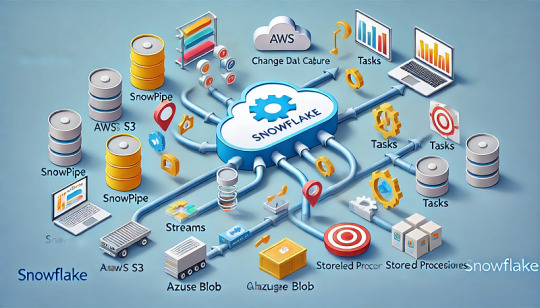
A guide to setting up automated data workflows with Snowflake.

Introduction

In today’s data-driven world, organizations need to process vast amounts of data efficiently. Snowflake, a cloud-based data platform, offers powerful automation features that help streamline workflows, reduce manual effort, and enhance data processing efficiency.

Automating data workflows in Snowflake is essential for:

Real-time data ingestion from various sources.

Incremental data processing using change data capture (CDC).

Scheduled data transformations for ETL/ELT pipelines.

Trigger-based workflows that respond to new data events.

This guide will walk you through Snowflake’s automation features, step-by-step implementation, and best practices to ensure optimal workflow execution.

Understanding Snowflake Automation Features

Snowflake provides several built-in automation tools to simplify data workflows:

1. Snowpipe: Automated Data Ingestion

What it does: Snowpipe enables continuous and automated loading of data from cloud storage (AWS S3, Azure Blob, or Google Cloud Storage) into Snowflake tables.

Key Benefits:

Near real-time data ingestion.

Cost-efficient pay-per-use pricing model.

Automatic triggering using cloud storage event notifications.

2. Streams: Change Data Capture (CDC) in Snowflake

What it does: Streams track inserts, updates, and deletes in a table, enabling incremental data processing.

Key Benefits:

Efficient CDC mechanism for ETL workflows.

Ensures only modified data is processed, reducing compute costs.

Works seamlessly with Snowflake Tasks for automation.

3. Tasks: Automating SQL Workflows

What it does: Snowflake Tasks allow scheduling and chaining of SQL queries, enabling sequential execution.

Key Benefits:

Automates transformations and incremental data loads.

Supports event-driven workflows.

Can be scheduled using cron expressions.

4. Stored Procedures: Automating Complex Business Logic

What it does: Stored procedures allow procedural execution of SQL and Python-based logic within Snowflake.

Key Benefits:

Enables advanced data processing beyond standard SQL queries.

Supports loops, conditions, and API calls.

Works well with Tasks and Streams for automation.

Step-by-Step Guide to Setting Up Automated Workflows in Snowflake

1. Automating Data Ingestion with Snowpipe

Step 1: Create an External Stage

sqlCREATE OR REPLACE STAGE my_s3_stage URL = 's3://my-bucket/data/' STORAGE_INTEGRATION = my_s3_integration;

Step 2: Define a File Format

sqlCREATE OR REPLACE FILE FORMAT my_csv_format TYPE = 'CSV' FIELD_OPTIONALLY_ENCLOSED_BY = '"';

Step 3: Create a Table for the Incoming Data

sqlCREATE OR REPLACE TABLE raw_data ( id INT, name STRING, created_at TIMESTAMP );

Step 4: Create and Configure Snowpipe

sqlCREATE OR REPLACE PIPE my_snowpipe AUTO_INGEST = TRUE AS COPY INTO raw_data FROM @my_s3_stage FILE_FORMAT = (FORMAT_NAME = my_csv_format);

✅ Outcome: This Snowpipe will automatically load new files from S3 into the raw_data table whenever a new file arrives.

2. Scheduling Workflows Using Snowflake Tasks

Step 1: Create a Task for Data Transformation

sqlCREATE OR REPLACE TASK transform_data_task WAREHOUSE = my_warehouse SCHEDULE = 'USING CRON 0 * * * * UTC' AS INSERT INTO transformed_data SELECT id, name, created_at, CURRENT_TIMESTAMP AS processed_at FROM raw_data;

✅ Outcome: This task runs hourly, transforming raw data into a structured format.

3. Tracking Data Changes with Streams for Incremental ETL

Step 1: Create a Stream on the Source Table

sqlCREATE OR REPLACE STREAM raw_data_stream ON TABLE raw_data;

Step 2: Create a Task to Process Changes

sqlCREATE OR REPLACE TASK incremental_etl_task WAREHOUSE = my_warehouse AFTER transform_data_task AS INSERT INTO processed_data SELECT * FROM raw_data_stream WHERE METADATA$ACTION = 'INSERT';

✅ Outcome:

The Stream captures new rows in raw_data.

The Task processes only the changes, reducing workload and costs.

4. Using Stored Procedures for Automation

Step 1: Create a Python-Based Stored Procedure

sqlCREATE OR REPLACE PROCEDURE cleanup_old_data() RETURNS STRING LANGUAGE PYTHON RUNTIME_VERSION = '3.8' HANDLER = 'cleanup' AS $$ def cleanup(session): session.sql("DELETE FROM processed_data WHERE processed_at < CURRENT_DATE - INTERVAL '30' DAY").collect() return "Cleanup Completed" $$;

Step 2: Automate the Procedure Execution Using a Task

sqlCREATE OR REPLACE TASK cleanup_task WAREHOUSE = my_warehouse SCHEDULE = 'USING CRON 0 0 * * * UTC' AS CALL cleanup_old_data();

✅ Outcome: The procedure automatically deletes old records every day.

Best Practices for Snowflake Automation

1. Optimize Task Scheduling

Avoid overlapping schedules to prevent unnecessary workload spikes.

Use AFTER dependencies instead of cron when chaining tasks.

2. Monitor and Troubleshoot Workflows

Use SHOW TASKS and SHOW PIPES to track execution status.

Check TASK_HISTORY and PIPE_USAGE_HISTORY for errors.

sqlSELECT * FROM SNOWFLAKE.INFORMATION_SCHEMA.TASK_HISTORY WHERE STATE != 'SUCCEEDED' ORDER BY COMPLETED_TIME DESC;

3. Cost Management

Choose the right warehouse size for executing tasks.

Pause tasks when not needed to save credits.

Monitor compute costs using WAREHOUSE_METERING_HISTORY.

4. Security Considerations

Grant least privilege access for tasks and Snowpipe.

Use service accounts instead of personal credentials for automation.

Encrypt sensitive data before ingestion.

Conclusion

Snowflake provides powerful automation tools to streamline data workflows, enabling efficient ETL, real-time ingestion, and scheduled transformations. By leveraging Tasks, Streams, Snowpipe, and Stored Procedures, you can build a fully automated data pipeline that is cost-effective, scalable, and easy to manage.

✅ Next Steps:

Experiment with multi-step task workflows.

Integrate Snowflake automation with Apache Airflow.

Explore event-driven pipelines using cloud functions.

WEBSITE: https://www.ficusoft.in/snowflake-training-in-chennai/

0 notes

dlbanalysis · 1 year ago

Text

Linear Regression 2.0 (Dummy Variables)

This is another Linear Regression post (using statsmodels) - but this time I wanted to talk about 'dummy variables'.

The overarching idea:

In the previous blog post at some point I mention about having multiple variables in our linear regression model that may (or may not) give us more explanatory power.

In this example we'll look at using a dummy variable (attendance) along with SAT score to give us a more precise GPA output.

The code:

Apologies in advance, I know this is incredibly messy - but I feel like the concept behind what's happening is more important than how it looks at the moment!

------------------------------------------------------------------------------ import numpy as np import pandas as pd import statsmodels.api as sm import matplotlib.pyplot as plt import seaborn as sns sns.set() raw_data = pd.read_csv('1.03.+Dummies.csv') data = raw_data.copy() data['Attendance'] = data['Attdance'].map({'Yes': 1, 'No': 0}) print(data.describe())

#REGRESSION # Following the regression equation, our dependent variable (y) is the GPA y = data ['GPA'] # Our independent variable (x) is the SAT score x1 = data [['SAT', 'Attendance']] # Add a constant. Esentially, we are adding a new column (equal in lenght to x), which consists only of 1s x = sm.add_constant(x1) # Fit the model, according to the OLS (ordinary least squares) method with a dependent variable y and an idependent x results = sm.OLS(y,x).fit() # Print a nice summary of the regression. results.summary()

plt.scatter(data['SAT'],y) yhat_no = 0.6439 + 0.0014*data['SAT'] yhat_yes = 0.8665 + 0.0014*data['SAT'] fig = plt.plot(data['SAT'],yhat_no, lw=2, c='#a50026') fig = plt.plot(data['SAT'],yhat_yes, lw=2, c='#006837') plt.xlabel('SAT', fontsize = 20) plt.ylabel('GPA', fontsize = 20) plt.scatter(data['SAT'],data['GPA'], c=data['Attendance'],cmap='RdYlGn')

# Define the two regression equations (one with a dummy = 1 [i.e 'Yes'], the other with dummy = 0 [i.e 'no']) yhat_no = 0.6439 + 0.0014*data['SAT'] yhat_yes = 0.8665 + 0.0014*data['SAT']

# Original regression line yhat = 0.0017*data['SAT'] + 0.275

#Plot the two regression lines fig = plt.plot(data['SAT'],yhat_yes, lw=2, c='#006837', label ='Attendance > 75%') fig = plt.plot(data['SAT'],yhat_no, lw=2, c='#a50026', label ='Attendance < 75%') # Plot the original regression line fig = plt.plot(data['SAT'],yhat, lw=3, c='#4C72B0', label ='original regression line') plt.legend(loc='lower right')

plt.xlabel('SAT', fontsize = 20) plt.ylabel('GPA', fontsize = 20) plt.show()

------------------------------------------------------------------------------

When you run the code, this is the graph you will get!

What am I looking at?

This graph is showing us students' SAT scores against their GPA. It is also showing us regression lines of attendance. In green, we have those students who attended more than 75% and in red, those students who had less than 75% attendance. We can clearly see that the students who had an attendance rate of over 75% are expected to achieve a higher GPA.

How was it done?

Obviously you could find that out by looking at the code - but I want to break it down into steps (for my own benefit in the future if nothing else!)

The first noticeable thing that is different from the previous blog post is we have loaded in the dataset into a variable called 'raw_data' (as opposed to 'data). This is because we have some extra work to do before we get started! *Just an aside here that in the 'Attendance' column we have 'Yes' or 'No' entries depending on whether or not the student has attendance rate of more than 75%.

The next two lines of code:

data = raw_data.copy()

data['Attendance'] = data['Attendance'].map({'Yes': 1, 'No': 0})

The first line will make a copy of our 'raw data' variable and call it 'data'. The next line maps all 'Yes' entries in the 'Attendance' column to 1 and all 'No' entries to 0. As below

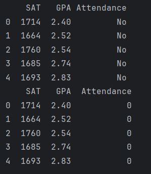
(we only see 5 entries here because both instances [i.e first section is the original and the second one is after the mapping] were printed with the 'data.head()' method).

3. The next thing we need to do is declare our dependent (y) and indedpendent (x1) variables, which are:

y = data ['GPA'] x1 = data [['SAT', 'Attendance']]

4. Once we have this it is the same as before, use statsmodels to create a constant and print some useful statistics!

x = sm.add_constant(x1) results = sm.OLS(y,x).fit() print(results.summary())

A couple of things to note here, the adjusted R-squared value (0.555) is a great improvement from the linear regression we peformed without attendance (0.399) [a note here to say that R-Squared and Adjusted R-Squared will get their own post one day!].

5. So, we can start constructing the equations now. So, our original one was: GPA = 0.275 + 0.0017*SAT

The model including the dummy variable is: GPA = 0.6429 + 0.0014*SAT + 0.2226*Dummy So now, we can split out this dummy variable into two equations (one that has a dummy value of '1' for the attendance greater than 75% and one that has a dummy value of '0' for the attendance less than 75%).

Attended (dummy = 1)

GPA = 0.8665 + 0.0014 * SAT

Did not attend (dummy = 0)

GPA = 0.6439 + 0.0014 * SAT

6. The next line of code is plotting the points in a scatter chart

7. After the points have been plotted we then define our regression lines (as mentioned above):

yhat_no = 0.6439 + 0.0014*data['SAT'] yhat_yes = 0.8665 + 0.0014*data['SAT']

8. Something that I wasn't sure about was one of the arguments in the plt.scatter function. This was the 'cmap='RdYlGn'' parameter. Obviously it is some sort of mapping (Red, Yellow, Green?) but the interesting thing about it was that originally it was 'cmap='RdYlGn_r'' - but I think this reversed the colours or something. Anyway, after I removed the '_r' I was able to display the <75% attendance data points in red which I thought was more intuitive.

9. For reference, perhaps it is a good idea to include our original regression line, this is:

yhat = 0.0017*data['SAT'] + 0.275 10. In the last few lines of code we are plotting the regression lines and giving them titles!

fig = plt.plot(data['SAT'],yhat_yes, lw=2, c='#006837', label ='Attendance > 75%') fig = plt.plot(data['SAT'],yhat_no, lw=2, c='#a50026', label ='Attendance < 75%') # Plot the original regression line fig = plt.plot(data['SAT'],yhat, lw=3, c='#4C72B0', label ='original regression line') plt.legend(loc='lower right')

plt.xlabel('SAT', fontsize = 20) plt.ylabel('GPA', fontsize = 20) plt.show()

So there you have it, that is our linear regression with a dummy variable. I thought that was really interesting. Quite a clever trick to convert categorical data into something numeric like that (but i suppose a binary outcome like 'yes' or 'no' is kind of easy enough I suppose - next time it'd be interesting to see how its done with something like eye colour [blue, green, brown, hazel etc].

0 notes

technoinuniverse-blog · 6 years ago

Photo

Boost your career Instant! This Tableau course will help you to build a successful career in Data Analyst domain and become a data analytics expert.

Learn more :- http://bit.ly/33NOIoE

#Tableau #Data_Analytic #data_visualization #raw_data #technical_skills #coding_knowledge #implementation #visualizations #discovering #uncovering_structure #databases #metadata

0 notes

twst-vcl · 5 years ago

Note

Where did you get the birthday greetings from?

To clarify, i've taken the raw_data from the game and unpacked them directly into the editor.. which mean, they're already in game..

13 notes · View notes

jayateerth · 5 years ago

Text

ML for Data Analysis - Week 1 Assignment

Age, Picture - Decision Tree for Regular Smoking (Run 2)

* Run 1 decision is not included because that was done for all the 24 explanatory variables and the split was not able to explain a specific non linear relationship among variables.

Decision tree analysis was performed to test nonlinear relationships among a series of explanatory variables and a binary, categorical response variable.

All possible separations (categorical) or cut points (quantitative) are tested. For the present analyses, the entropy “goodness of split” criterion was used to grow the tree and a cost complexity algorithm was used for pruning the full tree into a final subtree.

For Run -1, all the 24 explanatory variables were included as possible contributors to a classification tree model evaluating smoking (response variable), age, gender, (race/ethnicity) Hispanic, White, Black, Native American and Asian. Alcohol use, marijuana use, cocaine use, inhalant use, availability of cigarettes in the home, whether or not either parent was on public assistance, any experience with being expelled from school. alcohol problems, deviance, violence, depression, self-esteem, parental presence, parental activities, family connectedness, school connectedness and grade point average.

The deviance score was the first variable to separate the sample into two subgroups. Adolescents with a deviance score greater than 0.112 (range 0 to 2.8 –M=0.13, SD=0.209) were more likely to have experimented with smoking compared to adolescents not meeting this cutoff (18.6% vs. 11.2%).

Of the adolescents with deviance scores less than or equal to 0.112, a further subdivision was made with the dichotomous variable of alcohol use without supervision. Adolescents who reported having used alcohol without supervision were more likely to have experimented with smoking. Adolescents with a deviance score less than or equal to 0.112 who had never drank alcohol were less likely to have experimented with smoking.

The total model of run 1 classified 79% of the sample correctly,below is the confusion matrix.

[988, 154], [116, 115]]

For Run -1, following variables were used - Age, Alcohol use, marijuana use, cocaine use , availability of cigarettes in the home, and grade point average.

The total model of run 2 classified 78% of the sample correctly,below is the confusion matrix.

[[1308, 211], [ 186, 125]]

The code is included below.

# -*- coding: utf-8 -*- """ Created on Tue Mar 30, 17:15:34 2020 @author: Jayateerth Kulkarni

Python code for Classification using Decision Trees Week 1 Assignment - ML for Data Analysis """ """ OBJECTIVE - Decision tree analysis to test nonlinear relationships among a list of explanatory variables (Categorical & Quantitative) to classify categorical response variable. """

from pandas import Series, DataFrame import pandas as pd import numpy as np import os import matplotlib.pylab as plt

# the previous command where sklearn.cross-validation was used #is no longer applicable here hence changed to model selection

from sklearn.model_selection import train_test_split from sklearn.tree import DecisionTreeClassifier from sklearn.metrics import classification_report import sklearn.metrics

os.chdir("D:\ANALYTICS (DS, DAS ETC.)\R_Python\Python")

#Load the dataset

raw_data = pd.read_csv("tree_addhealth.csv") """ the dataframe.dropna() drops missing values for data frame""" data_clean = raw_data.dropna() """ the df.dtypes() shows the data type of the dataset""" data_clean.dtypes """ the df.describe() shows the summary of dataset""" data_clean.describe()

""" RUN-1 - with all variables""" #Split into training and testing sets

features = data_clean[['BIO_SEX','HISPANIC','WHITE','BLACK','NAMERICAN','ASIAN', 'age','ALCEVR1','ALCPROBS1','marever1','cocever1','inhever1','cigavail','DEP1', 'ESTEEM1','VIOL1','PASSIST','DEVIANT1','SCHCONN1','GPA1','EXPEL1','FAMCONCT','PARACTV', 'PARPRES']]

response = data_clean.TREG1

pred_train, pred_test, tar_train, tar_test = train_test_split(features, response, test_size=.3)

pred_train.shape pred_test.shape tar_train.shape tar_test.shape

#Build model on training data classifier=DecisionTreeClassifier() classifier=classifier.fit(pred_train,tar_train)

predictions=classifier.predict(pred_test)

sklearn.metrics.confusion_matrix(tar_test,predictions) sklearn.metrics.accuracy_score(tar_test, predictions)

#Displaying the decision tree from sklearn import tree #from StringIO import StringIO from io import StringIO #from StringIO import StringIO from IPython.display import Image out = StringIO() tree.export_graphviz(classifier, out_file=out) """ as pydotplus module not found we need to use the following conda install -c conda-forge pydotplus""" import pydotplus

graph=pydotplus.graph_from_dot_data(out.getvalue()) Image(graph.create_png()) graph.write_pdf("graph.pdf")

""" RUN-2 - with limited variables""" #Split into training and testing sets

features2 = data_clean[['age','ALCEVR1','marever1','cocever1', 'cigavail','GPA1']]

response2 = data_clean.TREG1

pred_train, pred_test, tar_train, tar_test = train_test_split(features2, response2, test_size=.4)

pred_train.shape pred_test.shape tar_train.shape tar_test.shape

#Build model on training data classifier=DecisionTreeClassifier() classifier=classifier.fit(pred_train,tar_train)

predictions=classifier.predict(pred_test)

sklearn.metrics.confusion_matrix(tar_test,predictions) sklearn.metrics.accuracy_score(tar_test, predictions)

#Displaying the decision tree from sklearn import tree #from StringIO import StringIO from io import StringIO #from StringIO import StringIO from IPython.display import Image out2 = StringIO() tree.export_graphviz(classifier, out_file=out2) """ as pydotplus module not found we need to use the following conda install -c conda-forge pydotplus""" import pydotplus

graph=pydotplus.graph_from_dot_data(out2.getvalue()) Image(graph.create_png()) graph.write_pdf("graph.pdf")

1 note · View note

jon-ting-data-manage-vis · 5 years ago

Text

Testing a Potential Moderator

Following previous visualizations and assessments done on the GapMinder dataset, the conclusion obtained seems to indicate that the oil consumption per person is significantly related to the residential electricity consumption per person. It would thus be interesting to test for a potential moderator between the variables. Urban population is chosen for this purpose.

The codes written for this program are shown below:

#############################################

# Import required libraries import pandas as pd import numpy as np import seaborn as sns import matplotlib as mpl import matplotlib.pyplot as plt import statsmodels.formula.api as smf import statsmodels.stats.multicomp as multi import scipy.stats

# Bug fix for display formats and change settings to show all rows and columns pd.set_option('display.float_format', lambda x:'%f'%x) pd.set_option('display.max_columns', None) pd.set_option('display.max_rows', None)

# Read in the GapMinder dataset raw_data = pd.read_csv('./gapminder.csv', low_memory=False)

# Report facts regarding the original dataset print("Facts regarding the original GapMinder dataset:") print("---------------------------------------") print("Number of countries: {0}".format(len(raw_data))) print("Number of variables: {0}\n".format(len(raw_data.columns))) print("All variables:\n{0}\n".format(list(raw_data.columns))) print("Data types of each variable:\n{0}\n".format(raw_data.dtypes)) print("First 5 rows of entries:\n{0}\n".format(raw_data.head())) print("=====================================\n")

# Choose variables of interest # var_of_int = ['country', 'incomeperperson', 'alcconsumption', 'co2emissions', # 'internetuserate', 'oilperperson', 'relectricperperson', 'urbanrate'] var_of_int = ['oilperperson', 'relectricperperson', 'urbanrate'] print("Chosen variables of interest:\n{0}\n".format(var_of_int)) print("=====================================\n")

# Code out missing values by replacing with NumPy's NaN data type data = raw_data[var_of_int].replace(' ', np.nan) print("Replaced missing values with NaNs:\n{0}\n".format(data.head())) print("=====================================\n")

# Cast the numeric variables to the appropriate data type then quartile split numeric_vars = var_of_int[:] for var in numeric_vars: data[var] = pd.to_numeric(data[var], downcast='float', errors='raise') print("Simple statistics of each variable:\n{0}\n".format(data.describe())) print("=====================================\n")

# Create secondary variables to investigate frequency distributions print("Separate continuous values categorically using secondary variables:") print("---------------------------------------") data['oilpp (tonnes)'] = pd.cut(data['oilperperson'], 4) oil_val_count = data.groupby('oilpp (tonnes)').size() oil_dist = data['oilpp (tonnes)'].value_counts(sort=False, dropna=True, normalize=True) oil_freq_tab = pd.concat([oil_val_count, oil_dist], axis=1) oil_freq_tab.columns = ['value_count', 'frequency'] print("Frequency table of oil consumption per person:\n{0}\n".format(oil_freq_tab))

data['relectricpp (kWh)'] = pd.cut(data['relectricperperson'], 2) elec_val_count = data.groupby('relectricpp (kWh)').size() elec_dist = data['relectricpp (kWh)'].value_counts(sort=False, dropna=True, normalize=True) elec_freq_tab = pd.concat([elec_val_count, elec_dist], axis=1) elec_freq_tab.columns = ['value_count', 'frequency'] print("Frequency table of residential electricity consumption per person:\n{0}\n".format(elec_freq_tab))

data['urbanr (%)'] = pd.cut(data['urbanrate'], 4) urb_val_count = data.groupby('urbanr (%)').size() urb_dist = data['urbanr (%)'].value_counts(sort=False, dropna=True, normalize=True) urb_freq_tab = pd.concat([urb_val_count, urb_dist], axis=1) urb_freq_tab.columns = ['value_count', 'frequency'] print("Frequency table of urban population:\n{0}\n".format(urb_freq_tab)) print("=====================================\n")

# Code in valid data in place of missing data for each variable print("Number of missing data in variables:") print("oilperperson: {0}".format(data['oilperperson'].isnull().sum())) print("relectricperperson: {0}".format(data['relectricperperson'].isnull().sum())) print("urbanrate: {0}\n".format(data['urbanrate'].isnull().sum())) print("=====================================\n")

print("Investigate entries with missing urbanrate data:\n{0}\n".format(data[['oilperperson', 'relectricperperson']][data['urbanrate'].isnull()])) print("Data for other variables are also missing for 90% of these entries.") print("Therefore, eliminate them from the dataset.\n") data = data[data['urbanrate'].notnull()] print("=====================================\n")

null_elec_data = data[data['relectricperperson'].isnull()].copy() print("Investigate entries with missing relectricperperson data:\n{0}\n".format(null_elec_data.head())) elec_map_dict = data.groupby('urbanr (%)').median()['relectricperperson'].to_dict() print("Median values of relectricperperson corresponding to each urbanrate group:\n{0}\n".format(elec_map_dict)) null_elec_data['relectricperperson'] = null_elec_data['urbanr (%)'].map(elec_map_dict) data = data.combine_first(null_elec_data) data['relectricpp (kWh)'] = pd.cut(data['relectricperperson'], 2) print("Replace relectricperperson NaNs based on their quartile group's median:\n{0}\n".format(data.head())) print("-------------------------------------\n")

null_oil_data = data[data['oilperperson'].isnull()].copy() oil_map_dict = data.groupby('urbanr (%)').median()['oilperperson'].to_dict() print("Median values of oilperperson corresponding to each urbanrate group:\n{0}\n".format(oil_map_dict)) null_oil_data['oilperperson'] = null_oil_data['urbanr (%)'].map(oil_map_dict) data = data.combine_first(null_oil_data) data['oilpp (tonnes)'] = pd.cut(data['oilperperson'], 4) print("Replace oilperperson NaNs based on their quartile group's median:\n{0}\n".format(data.head())) print("=====================================\n")

# Investigate the new frequency distributions print("Report the new frequency table for each variable:") print("---------------------------------------") oil_val_count = data.groupby('oilpp (tonnes)').size() oil_dist = data['oilpp (tonnes)'].value_counts(sort=False, dropna=True, normalize=True) oil_freq_tab = pd.concat([oil_val_count, oil_dist], axis=1) oil_freq_tab.columns = ['value_count', 'frequency'] print("Frequency table of oil consumption per person:\n{0}\n".format(oil_freq_tab))

elec_val_count = data.groupby('relectricpp (kWh)').size() elec_dist = data['relectricpp (kWh)'].value_counts(sort=False, dropna=True, normalize=True) elec_freq_tab = pd.concat([elec_val_count, elec_dist], axis=1) elec_freq_tab.columns = ['value_count', 'frequency'] print("Frequency table of residential electricity consumption per person:\n{0}\n".format(elec_freq_tab))

urb_val_count = data.groupby('urbanr (%)').size() urb_dist = data['urbanr (%)'].value_counts(sort=False, dropna=True, normalize=True) urb_freq_tab = pd.concat([urb_val_count, urb_dist], axis=1) urb_freq_tab.columns = ['value_count', 'frequency'] print("Frequency table of urban population:\n{0}\n".format(urb_freq_tab)) print("=====================================\n")

# Testing for moderator effect print("Testing for moderator effect:") print("-------------------------------------") print("Urban population as moderator:") urb1 = data[data['urbanr (%)'] == '(10.31, 32.8]'] urb2 = data[data['urbanr (%)'] == '(32.8, 55.2]'] urb3 = data[data['urbanr (%)'] == '(55.2, 77.6]'] urb4 = data[data['urbanr (%)'] == '(77.6, 100]'] print('Association between relectricperperson and oilperperson for urbanr (%) (10.31, 32.8]:\n{0}\n' .format(scipy.stats.pearsonr(urb1['relectricperperson'], urb1['oilperperson']))) print('Association between relectricperperson and oilperperson for urbanr (%) (32.8, 55.2]:\n{0}\n' .format(scipy.stats.pearsonr(urb2['relectricperperson'], urb2['oilperperson']))) print('Association between relectricperperson and oilperperson for urbanr (%) (55.2, 77.6]:\n{0}\n' .format(scipy.stats.pearsonr(urb3['relectricperperson'], urb3['oilperperson']))) print('Association between relectricperperson and oilperperson for urbanr (%) (77.6, 100]:\n{0}\n' .format(scipy.stats.pearsonr(urb4['relectricperperson'], urb4['oilperperson'])))

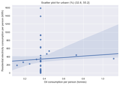
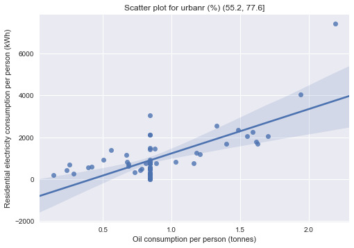
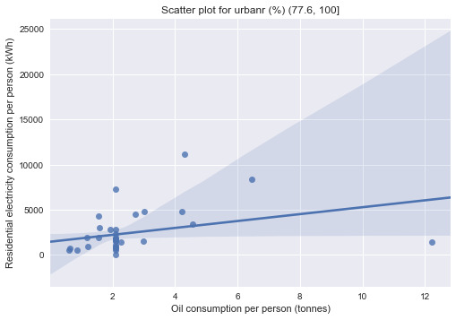
print("\nBivariate graphs:") print("-------------------------------------") sns.regplot(x='oilperperson', y='relectricperperson', data=urb1) plt.xlabel("Oil consumption per person (tonnes)") plt.ylabel("Residential electricity consumption per person (kWh)") plt.title("Scatter plot for urbanr (%) (10.31, 32.8]") plt.show() sns.regplot(x='oilperperson', y='relectricperperson', data=urb2) plt.xlabel("Oil consumption per person (tonnes)") plt.ylabel("Residential electricity consumption per person (kWh)") plt.title("Scatter plot for urbanr (%) (32.8, 55.2]") plt.show() sns.regplot(x='oilperperson', y='relectricperperson', data=urb3) plt.xlabel("Oil consumption per person (tonnes)") plt.ylabel("Residential electricity consumption per person (kWh)") plt.title("Scatter plot for urbanr (%) (55.2, 77.6]") plt.show() sns.regplot(x='oilperperson', y='relectricperperson', data=urb4) plt.xlabel("Oil consumption per person (tonnes)") plt.ylabel("Residential electricity consumption per person (kWh)") plt.title("Scatter plot for urbanr (%) (77.6, 100]") plt.show()

#############################################

The output of the program is as follow:

#############################################

Facts regarding the original GapMinder dataset: --------------------------------------- Number of countries: 213 Number of variables: 16

All variables: ['country', 'incomeperperson', 'alcconsumption', 'armedforcesrate', 'breastcancerper100th', 'co2emissions', 'femaleemployrate', 'hivrate', 'internetuserate', 'lifeexpectancy', 'oilperperson', 'polityscore', 'relectricperperson', 'suicideper100th', 'employrate', 'urbanrate']

Data types of each variable: country object incomeperperson object alcconsumption object armedforcesrate object breastcancerper100th object co2emissions object femaleemployrate object hivrate object internetuserate object lifeexpectancy object oilperperson object polityscore object relectricperperson object suicideper100th object employrate object urbanrate object dtype: object

First 5 rows of entries: country incomeperperson alcconsumption armedforcesrate \ 0 Afghanistan .03 .5696534 1 Albania 1914.99655094922 7.29 1.0247361 2 Algeria 2231.99333515006 .69 2.306817 3 Andorra 21943.3398976022 10.17 4 Angola 1381.00426770244 5.57 1.4613288

breastcancerper100th co2emissions femaleemployrate hivrate \ 0 26.8 75944000 25.6000003814697 1 57.4 223747333.333333 42.0999984741211 2 23.5 2932108666.66667 31.7000007629394 .1 3 4 23.1 248358000 69.4000015258789 2

internetuserate lifeexpectancy oilperperson polityscore \ 0 3.65412162280064 48.673 0 1 44.9899469578783 76.918 9 2 12.5000733055148 73.131 .42009452521537 2 3 81 4 9.99995388324075 51.093 -2

relectricperperson suicideper100th employrate urbanrate 0 6.68438529968262 55.7000007629394 24.04 1 636.341383366604 7.69932985305786 51.4000015258789 46.72 2 590.509814347428 4.8487696647644 50.5 65.22 3 5.36217880249023 88.92 4 172.999227388199 14.5546770095825 75.6999969482422 56.7

=====================================

Chosen variables of interest: ['oilperperson', 'relectricperperson', 'urbanrate']

=====================================

Replaced missing values with NaNs: oilperperson relectricperperson urbanrate 0 NaN NaN 24.04 1 NaN 636.341383366604 46.72 2 .42009452521537 590.509814347428 65.22 3 NaN NaN 88.92 4 NaN 172.999227388199 56.7

=====================================

Simple statistics of each variable: oilperperson relectricperperson urbanrate count 63.000000 136.000000 203.000000 mean 1.484085 1173.179199 56.769348 std 1.825090 1681.440430 23.844936 min 0.032281 0.000000 10.400000 25% 0.532542 203.652103 36.830000 50% 1.032470 597.136444 57.939999 75% 1.622737 1491.145233 74.209999 max 12.228645 11154.754883 100.000000

=====================================

Separate continuous values categorically using secondary variables: --------------------------------------- Frequency table of oil consumption per person: value_count frequency oilpp (tonnes) (0.0201, 3.0814] 58 0.920635 (3.0814, 6.13] 3 0.047619 (6.13, 9.18] 1 0.015873 (9.18, 12.229] 1 0.015873

Frequency table of residential electricity consumption per person: value_count frequency relectricpp (kWh) (-11.155, 5577.377] 132 0.970588 (5577.377, 11154.755] 4 0.029412

Frequency table of urban population: value_count frequency urbanr (%) (10.31, 32.8] 42 0.206897 (32.8, 55.2] 51 0.251232 (55.2, 77.6] 68 0.334975 (77.6, 100] 42 0.206897

=====================================

Number of missing data in variables: oilperperson: 150 relectricperperson: 77 urbanrate: 10

=====================================

Investigate entries with missing urbanrate data: oilperperson relectricperperson 43 nan nan 71 nan 0.000000 75 nan nan 121 nan nan 134 nan nan 143 nan nan 157 nan nan 170 nan nan 187 2.006515 1831.731812 198 nan nan

Data for other variables are also missing for 90% of these entries. Therefore, eliminate them from the dataset.

=====================================

Investigate entries with missing relectricperperson data: oilperperson relectricperperson urbanrate oilpp (tonnes) \ 0 nan nan 24.040001 NaN 3 nan nan 88.919998 NaN 5 nan nan 30.459999 NaN 8 nan nan 46.779999 NaN 12 nan nan 83.699997 NaN

relectricpp (kWh) urbanr (%) 0 NaN (10.31, 32.8] 3 NaN (77.6, 100] 5 NaN (10.31, 32.8] 8 NaN (32.8, 55.2] 12 NaN (77.6, 100]

Median values of relectricperperson corresponding to each urbanrate group: {'(10.31, 32.8]': 59.848274, '(32.8, 55.2]': 278.73962, '(55.2, 77.6]': 753.20978, '(77.6, 100]': 1741.4866}

Replace relectricperperson NaNs based on their quartile group's median: oilperperson relectricperperson urbanrate oilpp (tonnes) \ 0 nan 59.848274 24.040001 NaN 1 nan 636.341370 46.720001 NaN 2 0.420095 590.509827 65.220001 (0.0201, 3.0814] 3 nan 1741.486572 88.919998 NaN 4 nan 172.999222 56.700001 NaN

relectricpp (kWh) urbanr (%) 0 (-11.155, 5577.377] (10.31, 32.8] 1 (-11.155, 5577.377] (32.8, 55.2] 2 (-11.155, 5577.377] (55.2, 77.6] 3 (-11.155, 5577.377] (77.6, 100] 4 (-11.155, 5577.377] (55.2, 77.6]

-------------------------------------

Median values of oilperperson corresponding to each urbanrate group: {'(10.31, 32.8]': 0.079630107, '(32.8, 55.2]': 0.35917261, '(55.2, 77.6]': 0.84457392, '(77.6, 100]': 2.0878479}

Replace oilperperson NaNs based on their quartile group's median: oilperperson relectricperperson urbanrate oilpp (tonnes) \ 0 0.079630 59.848274 24.040001 (0.0201, 3.0814] 1 0.359173 636.341370 46.720001 (0.0201, 3.0814] 2 0.420095 590.509827 65.220001 (0.0201, 3.0814] 3 2.087848 1741.486572 88.919998 (0.0201, 3.0814] 4 0.844574 172.999222 56.700001 (0.0201, 3.0814]

=====================================

Report the new frequency table for each variable: --------------------------------------- Frequency table of oil consumption per person: value_count frequency oilpp (tonnes) (0.0201, 3.0814] 198 0.975369 (3.0814, 6.13] 3 0.014778 (6.13, 9.18] 1 0.004926 (9.18, 12.229] 1 0.004926

Frequency table of residential electricity consumption per person: value_count frequency (-11.155, 5577.377] 199 0.980296 (5577.377, 11154.755] 4 0.019704

Frequency table of urban population: value_count frequency (10.31, 32.8] 42 0.206897 (32.8, 55.2] 51 0.251232 (55.2, 77.6] 68 0.334975 (77.6, 100] 42 0.206897

=====================================

Testing for moderator effect: ------------------------------------- Urban population as moderator: Association between relectricperperson and oilperperson for urbanr (%) (10.31, 32.8]: (0.01366522, 0.93155224561464989)

Association between relectricperperson and oilperperson for urbanr (%) (32.8, 55.2]: (0.0682716, 0.63405606539354642)

Association between relectricperperson and oilperperson for urbanr (%) (55.2, 77.6]: (0.71694803, 6.1341947698015476e-12)

Association between relectricperperson and oilperperson for urbanr (%) (77.6, 100]: (0.32389528, 0.036392765827368875)

Bivariate graphs: -------------------------------------

#############################################

The data are separated into 4 groups according to the urban population quartile they belong to. Since both of the explanatory and response variables in this experiment are quantitative, correlation coefficients are computed for the test.

The test showed that only correlation coefficients between residential electricity consumption per person and oil consumption per person for country subgroups with higher urban population (>55.2%) are statistically significant (p=6.1341947698015476e-12 and p=0.036392765827368875 respectively). This means that the finding from the previous assessments that oil consumption per person is strongly correlated with residential electricity consumption is only applicable to countries with relatively high urban population (i.e. urban population is acting as a moderator between the 2 variables in question).

The scatter plots confirmed the findings as the regression lines for the subgroups with lower urban population are relatively flat compared to those with higher urban population. The oil consumption per person was most correlated to residential electricity consumption per person for subgroup with urban population between 55.2-77.6%.

0 notes

recreationblog · 5 years ago

Text

raw_data

0 notes

netmetic · 5 years ago

Text

Using Solace PubSub+ with OneTick Time Series Database

OneTick is a time-series database that is heavily used in financial services by hedge funds, brokerages and investment banks. OneMarketData, the maker of OneTick, describes it as “the premier enterprise-wide solution for tick data capture, streaming analytics, data management and research.” OneTick captures, compresses, archives, and provides uniform access to global historical data, up to and including the latest tick.

I myself have used OneTick for almost 5 years and found it to be a very nicely packaged solution thanks to built-in collectors for popular feeds such as Reuters’ Elektron and Bloomberg’s MBPIPE. OneTick also comes with a GUI that makes it easy for non-developers, such as researchers and portfolio managers, to write advanced queries using pre-built event processors (EPs). The GUI can be used to design queries that you can run from the GUI or APIs that OneTick supports, such as Python.

For example, here is a simple query that would select trade data for AAPL where price is greater than or equal to 21.5 (data is from 2003). In SQL, this would be select * from <database_name> where symbol="AAPL" and price >= 21.5.

OneTick comes with a DEMO database that I will be using for my examples. Here is what the query looks like in OneTick GUI:

When you run this query, you will see the result in OneTick’s GUI.

That’s useful information, but what if…

You wanted to stream this data to your real-time event-driven applications?

You wanted to publish the data once and have many recipients get it?

You wanted to let downstream applications retrieve data via open APIs and message protocols?

Solace PubSub+ Event Broker makes all of that possible!

How PubSub+ Can Help OneTick Developers

Here are some of the many ways OneTick developers can leverage PubSub+:

Consume data from a central distribution bus Many financial companies capture market data from external vendors and distribute it to their applications internally via PubSub+. OneTick developers can now natively consume the data and store it for later use.

Distribute data from OneTick to other applications Instead of delivering data individually to each client/application, OneTick developers can leverage pub/sub messaging pattern to publish data once and have it consumed multiple times.

Migrate to the cloud Have you been thinking about moving your applications and/or data to the cloud? With PubSub+ you can easily give cloud-native applications access to your high-volume data stored in on-prem OneTick instance using an event mesh.

Easier integration PubSub+ supports open APIs and protocols which make it a perfect option for integrating applications. Your applications can now use a variety of APIs to publish to and subscribe data from OneTick.

Replay messages Are you tired of losing critical data such as order flows when your applications crash? Replay functionality helps protect applications by giving them the ability to correct database issues they might have arising from events such as misconfiguration, application crashes, or corruption, by redelivering data to the applications.

Automate notifications It’s always a challenge to ensure all of the consumers are aware of any data issues whether it be an exchange outage leading to data gaps or delay in an ETL process. With PubSub+, OneTick developers can automate the publication of notifications related to their databases and broadcast it to the interested subscribers.

Running an Instance of PubSub+ Event Broker

In the rest of this post, I am going to show you how you can take data from your OneTick database and publish it to PubSub+, and vice versa. To follow along you will need access to an instance of PubSub+. If you don’t, there are two free ways to set up an instance:

Install a Docker container locally or in the cloud

Set up a dev instance on Solace Cloud (easiest way to get started)

Please post on Solace Community if you have any issues setting up an instance.

Publishing data from OneTick to PubSub+

OneTick makes it extremely easy for you to publish data to PubSub+ by simply using a built-in event processor (EP). The EP is called WRITE_TO_SOLACE and is part of OneTick’s Output Adapters (see OneTick docs: docs/ep_guide/EP/OutputAdapters.htm) which contains other EPs such as WRITE_TEXT, WRITE_TO_RAW, and WRITE_TO_ONETICK_DB.

To publish results of our previous query to PubSub+, we would simply add WRITE_TO_SOLACE EP at the end of our query and fill in appropriate connection and other details. Here is what the EP parameters look like:

You can find details about the WRITE_TO_SOLACE EP and its parameters in OneTick docs (docs/ep_guide/EP/OMD/WRITE_TO_SOLACE.htm).

The first few fields in the EP are for your PubSub+ connection details such as HOSTNAME, VPN, USERNAME, and PASSWORD.

The EP supports both direct and guaranteed message delivery. Direct messages are suitable for high throughput/low latency use cases such as market data distribution, and guaranteed messages are appropriate for critical messages that can’t be lost, such as order flow. You can learn more about the two delivery modes here.

The EP also allows you to specify the ENDPOINT you would like to publish data to, and the ENDPOINT_TYPE where you can specify if it is a topic or a queue. Publishing to a topic supports the pub/sub messaging pattern where your application publishes once to the topic and many applications can subscribe to that topic. On the other hand, publishing to a queue is point-to-point messaging because only the consumer binding to that specific queue can consume data published to it. Needless to say, we encourage clients to use the pub/sub messaging pattern as it provides more flexibility.

For this example today, I will publish to this topic: EQ/US/<security_name; such as EQ/US/AAPL.

Finally, you will notice that the EP allows users to specify the message format via MSG_FORMAT field. Currently, you can only pick from NAME_VALUE_PAIRS and BINARY, but OneTick will support additional message formats soon.

Configuring Subscriptions on PubSub+ Broker

Before publishing data to PubSub+, you need to determine how it will be consumed. Applications can either subscribe directly to the topic we are publishing to, or map the topic(s) to a queue and consume them from there. Using a queue introduces persistence so if your consumer disconnects abruptly, your messages won’t be lost. For our example, we will consume from a queue called onetick_queue that I have created from PubSub+’s UI:

PubSub+ allows you to map one or many topics to a queue, which means your consumer only needs to worry about binding to one queue and it can have messages being published to different topics ordered and delivered to that queue.

Additionally, PubSub+ also supports rich hierarchical topics and wildcards so you can dynamically filter the data you are interested in consuming. PubSub+ supports two wildcards: * lets you abstract away one topic level, and > lets you abstract away one or more levels. So, if you wanted to subscribe to all the data for equities, you can simply subscribe to EQ/> and if you wanted to subscribe to data for AAPL from different regions/venues, you could subscribe to EQ/*/AAPL.

You can learn more about Solace topics and wildcards here.

I have subscribed my queue to topic: EQ/US/AAPL.

With that done, you’re ready to run the query!

Once you have run your OneTick query, go to the PubSub+ UI and note that messages are in the queue.

As you can see, there are 8,278 messages in our queue.

This is how easy it is to publish messages from OneTick to PubSub+!

Writing Data from PubSub+ to OneTick

Now it’s time to consume data from PubSub+ and write it to a OneTick database. To be efficient you can use the data in the onetick_queue to write to OneTick db.

To read data from PubSub+, OneTick provides the omd::OneTickSolaceConsumer interface via its C++ API. Use this interface to connect to a Solace broker, make subscriptions, process received messages, and propagate those messages to the Custom Serialization interface.

To make things simple for us, OneTick distribution comes with a C++ example (examples/cplusplus/solace_consumer.cpp) that shows you how to do that. You can go through the code to see how to use the OneTick/Solace API but for the purpose of this post, we will simply run the code. However, before we can write the data from PubSub+ to a OneTick database, we need to create/configure that database.

I have created a database called solace by following these steps:

Create data directory for our database. I have created mine at: C:/omd/one_market/data/data/solace

Create a database entry in your locator file. Here is my locator entry for solace db:

Now that we have our database configured, we are ready to run our sample code. We will need to provide the following details to run the example:

PubSub+ connection details: host:port, username, password, vpn

endpoint: which topic/queue to subscribe to

OneTick db: name of database we will be writing data to

If the queue doesn’t exist, our code will administratively create it and map topics to it. In our case, we already have a queue (onetick_queue) that we will be consuming from.

As soon as we run the example, it will consume all the messages from the queue:

C:\omd\one_market_data\one_tick\examples\cplusplus>solace_consumer.exe -hostname <host_name>.messaging.solace.cloud -username <username> -password <password> -vpn himanshu-demo-dev -queue onetick_queue -dbname solace 20200509021426 INFO: Relevant section in locator <DB DAY_BOUNDARY_TZ="GMT" ID="solace" SYMBOLOGY="SOLACE" TIME_SERIES_IS_COMPOSITE="YES" > <LOCATIONS > <LOCATION ACCESS_METHOD="file" END_TIME="20300101000000" LOCATION="C:\omd\data\solace" START_TIME="20000101000000" /> </LOCATIONS> <RAW_DATA > <RAW_DB ID="PRIMARY" PREFIX="solace." > <LOCATIONS > <LOCATION ACCESS_METHOD="file" END_TIME="20300101000000" LOCATION="C:\omd\data\solace\raw_data" MOUNT="mount1" START_TIME="20000101000000" /> </LOCATIONS> </RAW_DB> </RAW_DATA> </DB>

After running the example, you will notice new raw data files have been created:

C:\omd\data\solace\raw_data>dir Directory of C:\omd\data\solace\raw_data 05/11/2020 05:41 PM <DIR> . 05/11/2020 05:41 PM <DIR> .. 05/11/2020 05:41 PM 245,644 solace.mount1.20200511214039 05/11/2020 05:41 PM 0 solace_mount1_lock 2 File(s) 245,644 bytes 2 Dir(s) 172,622,315,520 bytes free

Now, we need to run OneTick’s native_loader_daily.exe to archive the data:

C:\omd\one_market_data\one_tick\bin>native_loader_daily.exe -dbname solace -datadate 20200511 20200511214237 INFO: Native daily loader started 20200511214237 INFO: BuildNumber 20200420120000 Command and arguments: native_loader_daily.exe -dbname solace -datadate 20200511 ... 20200511214237 INFO: Picked up file C:\omd\data\solace\raw_data/solace.mount1.20200511214039 in raw db PRIMARY 20200511214237 INFO: Total processed messages: 8,468 (1,721,228 bytes) 20200511214237 INFO: Messages processed in last 0.046 seconds: 8,468 (1,721,228 bytes) at 184,652.958 msg/s (37,533,046.948 bytes/s) 20200511214237 INFO: Last measured message latency: NaN 20200511214237 INFO: Total processed messages: 8,468 (1,721,228 bytes) 20200511214237 INFO: Messages processed in last 0.005 seconds: 0 (0 bytes) at 0.000 msg/s (0.000 bytes/s) 20200511214237 INFO: Last measured message latency: NaN 20200511214237 INFO: persisting sorted batch 20200511214237 INFO: done persisting sorted batch 20200511214237 INFO: done persisting sorted batches for database solace, starting phase 2 of database load. Total symbols to load: 1, number of batches: 1 20200511214237 INFO: beginning sorted files cleanup 20200511214237 INFO: done with sorted files cleanup 20200511214237 INFO: loading index file; total records: 1 20200511214237 INFO: loading symbol file 20200511214237 INFO: renaming old archive directory, if exists 20200511214237 INFO: Load Complete for database solace for 20200511 Total ticks 8278 Total symbols 1 20200511214237 INFO: Processing time: 1

As you can see, 8,278 ticks have been archived – which is the same number of messages that were in the queue. You can now go to OneTick GUI and query the data from solace db:

That’s it!

I’ve shown you how easy it is to publish data from OneTick to PubSub+, read it back, and write to a OneTick database.

We are excited to have OneTick users like yourself take advantage of features like rich hierarchical topics, wildcards, support for open APIs and protocols and the dynamic message routing that enables event mesh.

If you would like to learn more about the API, please reach out to your OneTick account manager or support. If you would like to learn more about how to get started with PubSub+, please reach out to us here or check out our Solace with OneTick page.

The post Using Solace PubSub+ with OneTick Time Series Database appeared first on Solace.

Using Solace PubSub+ with OneTick Time Series Database published first on https://jiohow.tumblr.com/

0 notes