#Stochastics For Derivatives Modelling Project Help | Explore Tumblr posts and blogs

govindhtech · 16 days ago

Text

Pauli Propagation: A Novel Algorithm for Quantum Simulation

Introduction to Quantum Simulation Algorithms

Understanding complex physical processes is revolutionised by quantum computing. Due to exponential state space expansion, classical systems cannot simulate quantum systems, one of quantum technology’s most powerful applications. Because Hilbert spaces are so huge, conventional simulators struggle to represent quantum processes.

Pauli Propagation, a cutting-edge algorithm, models quantum systems in a scalable, accurate, and effective manner, notably noisy intermediate-scale quantum (NISQ) devices. Pauli Propagation uses stabiliser formalism and Pauli operator structure to achieve a sophisticated balance between quantum realism and classical efficiency.

Pauli Propagation—What?

The hybrid classical-quantum approach Pauli Propagation uses Pauli operators to express the state and its evolution to mimic quantum state evolution. Pauli Propagation simplifies the problem and reduces processing cost, unlike brute-force simulations that use complex matrix operations.

The program propagates Pauli strings over quantum circuits using classical principles derived from Clifford gates and non-Clifford perturbations, representing quantum states as linear combinations of these strings. This method saves resources and permits accurate modelling of Clifford circuits with few non-Clifford parts.

Pauli Operators in Quantum Simulation

The Pauli basis, consisting of {I, X, Y, Z} matrices, is the basis of Pauli Propagation. It provides a complete orthonormal basis for Hermitian operators on qubits. Extended density matrices and quantum operations in Pauli matrices make the simulation more structured and less computationally intensive.

Every quantum state is basically a sum of weighted Pauli strings, and measurements and gates influence the evolution of these strings. This method simplifies simulation by sparsely representing the quantum system and reducing full density matrix evolution.

Pauli Propagation Improves Efficiency

Compatible Clifford Circuit

Pauli Propagation works well in Clifford circuits, where Pauli operators stay inside the Pauli group under conjugation. This allows the algorithm to simulate quantum state movement through these circuits without exponentially increasing complexity.

Non-Clifford Elements Sampling

Simulating circuits using non-Clifford gates (like T gates) is tricky. Pauli Propagation uses Monte Carlo sampling to approximate non-Clifford gates. These samples accurately estimate observable expectation values, enabling near-exact simulations with low overhead.

Noise modelling

Real-world quantum devices are noisy. Pauli Propagation works with Lindbladian evolution, depolarising noise, and other quantum error models. By propagating error channels and quantum states, the method improves quantum algorithm dependability and performance forecasts on existing hardware.

Mathematical Pauli Propagation Formula

Define ρ as a quantum state:

ρ = ∑_i a_i P_i, where P_i are Pauli strings and a_i are real coefficients.

A single gate U affects ρ as: ρ’ = UρU† = ∑_i a_i U P_i U†

When U is a Clifford gate, propagation can be calculated efficiently as U P_i U† remains a Pauli operator. Importance sampling and stochastic trace estimation estimate non-Clifford process evolution.

The program enhances measurement outputs by projecting ρ onto a preferred foundation and adjusts coefficients accordingly.

Pauli Propagation Applications

Simulating quantum error correction

By simulating the effect of noise on error-correcting codes and modelling quantum circuits, Pauli Propagation helps evaluate novel quantum hardware and protocols’ fault tolerance.

Quantum Device Benchmarking

The method may simulate quantum volume, randomised benchmarking, and other hardware benchmarking measures to evaluate platforms or configurations.

Physics and Quantum Chemistry

Fermionic systems sometimes require complex operations that are difficult to express classically. Pauli Propagation simplifies these procedures by transforming them into classically computed Pauli string manipulations.

Variable Quantum Algorithms

Variational Quantum Eigensolver (VQE) and Quantum Approximate Optimisation Algorithm (QAOA) require Hamiltonian expectation values. Pauli Propagation can calculate these values accurately without complete quantum state tomography.

With its stabiliser formalism strengths and approximate techniques for non-Clifford circuits, Pauli Propagation fills a major need. This hybrid simulator is faster and more accurate that others.

Future Pauli-Based Simulation Developments Simulation tools must adapt to quantum hardware improvements. Future Pauli Propagation improvements may include:

Non-Clifford gates can be more accurate with adaptive sampling.

To manage complicated quantum systems, hybrid GPU-accelerated computation is used.

Quantum compiler integration: Circuit rewriting and dynamic optimisation.

These advances aim to bridge the gap between hardware restrictions and quantum algorithms.

In conclusion

Pauli Propagation revolutionised quantum simulation. Using Pauli operators’ algebraic structure and standard sampling methods, realistic quantum circuits can be reproduced correctly, efficiently, and scalable. Its compatibility with noise modelling, non-Clifford circuits, and hardware benchmarking makes it vital for NISQ-era researchers and engineers.

Whether you’re evaluating variational algorithms, revolutionary quantum error-correcting codes, or quantum hardware, Pauli Propagation has the accuracy and versatility you need.

#PauliPropagation #QuantumSimulation #Hilbertspaces #noisyintermediatescalequantum #quantumalgorithms #News #Technews #Technology #Technologynews #Technologytrends #Govindhtech

0 notes

sciforce · 5 years ago

Text

White Box AI: Interpretability Techniques

While in the previous article of the series we introduced the notion of White Box AI and explained different dimensions of interpretability, in this post we’ll be more practice-oriented and turn to techniques that can make algorithm output more explainable and the models more transparent, increasing trust in the applied models.

The two pillars of ML-driven predictive analysis are data and robust models, and these are the focus of attention in increasing interpretability. The first step towards White Box AI is data visualization because seeing your data will help you to get inside your dataset, which is a first step toward validating, explaining, and trusting models. At the same time, having explainable white-box models with transparent inner workings, followed by techniques that can generate explanations for the most complex types of predictive models such as model visualizations, reason codes, and variable importance measures.

Data Visualization

As we remember, good data science always starts with good data and with ensuring its quality and relevance for subsequent model training.

Unfortunately, most datasets are difficult to see and understand because they have too many variables and many rows. Plotting many dimensions is technically possible, but it does not improve the human understanding of complex datasets. Of course, there are numerous ways to visualize datasets and we discussed them in our dedicated article. However, in this overview, we’ll rely on the experts’ opinions and stick to those selected by Hall and Gill in their book “An Introduction to Machine Learning Interpretability”.

Most of these techniques have the capacity to illustrate all of a data set in just two dimensions, which is important in machine learning because most ML algorithms would automatically model high-degree interactions between multiple variables.

Glyphs

Glyphs are visual symbols used to represent different values or data attributes with the color, texture, or alignment. Using bright colors or unique alignments for events of interest or outliers is a good method for making important or unusual data attributes clear in a glyph representation. Besides, when arranged in a certain way, glyphs can be used to represent rows of a data set. In the figure below, each grouping of four glyphs can be either a row of data or an aggregated group of rows in a data set.

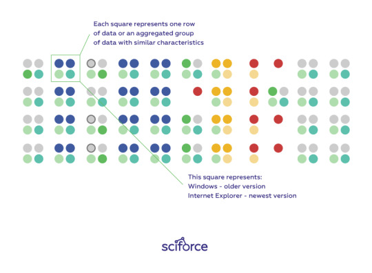
Figure 1. Glyphs arranged to represent many rows of a data set. Image courtesy of Ivy Wang and the H2O.ai team.

Correlation Graphs

A correlation graph is a two-dimensional representation of the relationships (i.e. correlation) in a data set. Even data sets with tens of thousands of variables can be displayed in two dimensions using this technique.

For the visual simplicity of correlation graphs, absolute weights below a certain threshold are not displayed. The node size is determined by a node’s number of connections (node degree), its color is determined by a graph community calculation, and the node position is defined by a graph force field algorithm. Correlation graphs show groups of correlated variables, help us identify irrelevant variables, and discover or verify important relationships that machine learning models should incorporate.

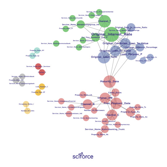
Figure 2. A correlation graph representing loans made by a large financial firm. Figure courtesy of Patrick Hall and the H2O.ai team.

In a supervised model built for the data represented in the figure above, we would expect variable selection techniques to pick one or two variables from the light green, blue, and purple groups, we would expect variables with thick connections to the target to be important variables in the model, and we would expect a model to learn that unconnected variables like CHANNEL_Rare not very important.

2-D projections

Of course, 2-D projection is not merely one technique and there exist any ways and techniques for projecting the rows of a data set from a usually high-dimensional original space into a more visually understandable 2- or 3-D space two or three dimensions, such as:

Principal Component Analysis (PCA)

Multidimensional Scaling (MDS)

t-distributed Stochastic Neighbor Embedding (t-SNE)

Autoencoder networks

Data sets containing images, text, or even business data with many variables can be difficult to visualize as a whole. These projection techniques try to represent the rows of high-dimensional data projecting them into a representative low-dimensional space and visualizing using the scatter plot technique. A high-quality projection visualized in a scatter plot is expected to exhibit key structural elements of a data set, such as clusters, hierarchy, sparsity, and outliers.

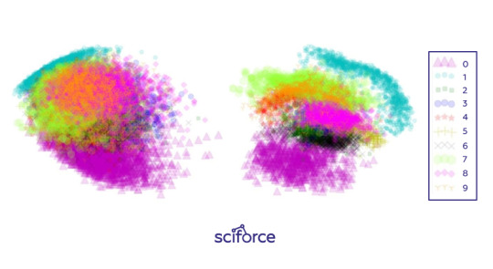
Figure 3. Two-dimensional projections of the 784-dimensional MNIST data set using (left) Principal Components Analysis (PCA) and (right) a stacked denoising autoencoder. Image courtesy of Patrick Hall and the H2O.ai team.

Projections can add trust if they are used to confirm machine learning modeling results. For instance, if known hierarchies, classes, or clusters exist in training or test data sets and these structures are visible in 2-D projections, it is possible to confirm that a machine learning model is labeling these structures correctly. Additionally, it shows if similar attributes of structures are projected relatively near one another and different attributes of structures are projected relatively far from one another. Such results should also be stable under minor perturbations of the training or test data, and projections from perturbed versus non-perturbed samples can be used to check for stability or for potential patterns of change over time.

Partial dependence plots

Partial dependence plots show how ML response functions change based on the values of one or two independent variables, while averaging out the effects of all other independent variables. Partial dependence plots with two independent variables are particularly useful for visualizing complex types of variable interactions between the independent variables. They can be used to verify monotonicity of response functions under monotonicity constraints, as well as to see the nonlinearity, non-monotonicity, and two-way interactions in very complex models. They can also enhance trust when displayed relationships conform to domain knowledge expectations. Partial dependence plots are global in terms of the rows of a data set, but local in terms of the independent variables.

Individual conditional expectation (ICE) plots, a newer and less spread adaptation of partial dependence plots, can be used to create more localized explanations using the same ideas as partial dependence plots.

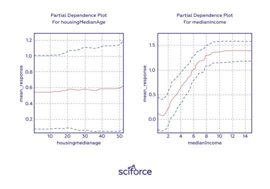
Figure 4. One-dimensional partial dependence plots from a gradient boosted tree ensemble model of the California housing data set. Image courtesy Patrick Hall and the H2O.ai team.

Residual analysis

Residuals refer to the difference between the recorded value of a dependent variable and the predicted value of a dependent variable for every row in a data set. In theory, the residuals of a well-fit model should be randomly distributed because good models will account for most phenomena in a data set, except for random error. Therefore, if models are producing randomly distributed residuals, this is an indication of a well-fit, dependable, trustworthy model. However, if strong patterns are visible in plotted residuals, there are problems with your data, your model, or both. Breaking out a residual plot by independent variables can additionally expose more granular information about residuals and assist in reasoning through the cause of non-random patterns.

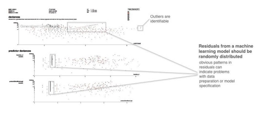
Figure 5. Screenshot from an example residual analysis application. Image courtesy of Micah Stubbs and the H2O.ai team.

Seeing structures and relationships in a data set makes those structures and relationships easier to understand and makes up a first step to knowing if a model’s answers are trustworthy.

Techniques for Creating White-Box Models

Decision trees

Decision trees, predicting the value of a target variable based on several input variables, are probably the most obvious way to ensure interpretability. They are directed graphs in which each interior node corresponds to an input variable. Each terminal node or leaf node represents a value of the target variable given the values of the input variables represented by the path from the root to the leaf. The major benefit of decision trees is that they can reveal relationships between the input and target variable with “Boolean-like” logic and they can be easily interpreted by non-experts by displaying them graphically. However, decision trees can create very complex nonlinear, nonmonotonic functions. Therefore, to ensure interpretability, they should be restricted to shallow depth and binary splits.

eXplainable Neural Networks

In contrast to decision trees, neural networks are often considered the least transparent of black-box models. However, the recent work in XNN implementation and explaining artificial neural network (ANN) predictions may render that characteristic obsolete. Many of the breakthroughs in ANN explanation were made possible thanks to the straightforward calculation of derivatives of the trained ANN response function with regard to input variables provided by deep learning toolkits such as Tensorflow. With the help of such derivatives, the trained ANN response function prediction can be disaggregated into input variable contributions for any observation. XNNs can model extremely nonlinear, nonmonotonic phenomena or they can be used as surrogate models to explain other nonlinear, non-monotonic models, potentially increasing the fidelity of global and local surrogate model techniques.

Monotonic gradient-boosted machines (GBMs)

Gradient boosting is an algorithm that produces a prediction model in the form of an ensemble of weak prediction models, typically decision trees. Used for regression and classification tasks, it is potentially appropriate for most traditional data mining and predictive modeling applications, even in regulated industries and for consistent reason code generation provided it builds monotonic functions. Monotonicity constraints can improve GBMs interpretability by enforcing a uniform splitting strategy in constituent decision trees, where binary splits of a variable in one direction always increase the average value of the dependent variable in the resultant child node, and binary splits of the variable in the other direction always decrease the average value of the dependent variable in the other resultant child node. Understanding is increased by enforcing straightforward relationships between input variables and the prediction target. Trust is increased when monotonic relationships, reason codes, and detected interactions are parsimonious with domain expertise or reasonable expectations.

Alternative regression white-box modeling approaches

There exist many modern techniques to augment traditional, linear modeling methods. Such models as elastic net, GAM, and quantile regression, usually produce linear, monotonic response functions with globally interpretable results similar to traditional linear models but with a boost in predictive accuracy.

Penalized (elastic net) regression

As an alternative to old-school regression models, penalized regression techniques usually combine L1/LASSO penalties for variable selection purposes and Tikhonov/L2/ridge penalties for robustness in a technique known as elastic net. Penalized regression minimizes constrained objective functions to find the best set of regression parameters for a given data set that would model a linear relationship and satisfy certain penalties for assigning correlated or meaningless variables to large regression coefficients. For instance, L1/LASSO penalties drive unnecessary regression parameters to zero, selecting only a small, representative subset of parameters for the regression model while avoiding potential multiple comparison problems. Tikhonov/L2/ridge penalties help preserve parameter estimate stability, even when many correlated variables exist in a wide data set or important predictor variables are correlated. Penalized regression is a great fit for business data with many columns, even data sets with more columns than rows, and for data sets with a lot of correlated variables.

Generalized Additive Models (GAMs)

Generalized Additive Models (GAMs) hand-tune a tradeoff between increased accuracy and decreased interpretability by fitting standard regression coefficients to certain variables and nonlinear spline functions to other variables. Also, most implementations of GAMs generate convenient plots of the fitted splines. That can be used directly in predictive models for increased accuracy. Otherwise, you can eyeball the fitted spline and switch it out for a more interpretable polynomial, log, trigonometric or other simple function of the predictor variable that may also increase predictive accuracy.

Quantile regression

Quantile regression is a technique that tries to fit a traditional, interpretable, linear model to different percentiles of the training data, allowing you to find different sets of variables with different parameters for modeling different behavior. While traditional regression is a parametric model and relies on assumptions that are often not met. Quantile regression makes no assumptions about the distribution of the residuals. It lets you explore different aspects of the relationship between the dependent variable and the independent variables.

There are, of course, other techniques, both based on applying constraints on regression and generating specific rules (like in OneR or RuleFit approaches). We encourage you to explore possibilities for enhancing model interpretability for any algorithm you choose and which is the most appropriate for your task and environment.

Evaluation of Interpretability

Finally, to ensure that the data and the trained models are interpretable, it is necessary to have robust methods for interpretability evaluation. However, with no real consensus about what interpretability is in machine learning, it is unclear how to measure it. Doshi-Velez and Kim (2017) propose three main levels for the evaluation of interpretability:

Application level evaluation (real task)

Essentially, it is putting the explanation into the product and having it tested by the end user. This requires a good experimental setup and an understanding of how to assess quality. A good baseline for this is always how good a human would be at explaining the same decision.

Human level evaluation (simple task)

It is a simplified application-level evaluation. The difference is that these experiments are not carried out with the domain experts, but with laypersons in simpler tasks like showing users several different explanations and letting them choose the best one. This makes experiments cheaper and it is easier to find more testers.

Function level evaluation (proxy task)

This task does not require humans. This works best when the class of model used has already been evaluated by humans. For example, if we know that end users understand decision trees, a proxy for explanation quality might be the depth of the tree with shorter trees having a better explainability score. It would make sense to add the constraint that the predictive performance of the tree remains good and does not decrease too much compared to a larger tree.

Most importantly, you should never forget that interpretability is not for machines but for humans, so the end users and their perception of data and models should always be in the focus of your attention. And humans prefer short explanations that contrast the current situation with a situation in which the event would not have occurred. Explanations are social interactions between the developer and the end user and it should always account for the social (and legal) context and the user’s expectations.

#artificial intelligence #machine learning #deep learning #data science #data visualization

3 notes · View notes

statisticshomeworktutors-blog · 7 years ago

Text

Stochastics For Derivatives Modelling Assignment Homework Help

https://www.statisticshomeworktutors.com/Stochastics-for-Derivatives-Modelling-Assignment-Help.php

If you are writing Derivatives Modelling Assignment, it becomes a tedious task for students to research analytically for assignments along with studying for their particular courses. This is not only difficult but a time-consuming task as well and this is why Statisticshomeworktutors procures assistance considering the quality required. We apprehend the value of the assignment grades for students and this is why we always maintain innovation and quality within the content. We have a global presence as our subject matter experts are highly qualified academically and professionally from different countries and so are the students and professionals.

#Stochastics For Derivatives Modelling Assignment Homework Help #Stochastics For Derivatives Modelling Assignment Help #Stochastics For Derivatives Modelling Homework Help #Stochastics For Derivatives Modelling Online Help #Stochastics For Derivatives Modelling Project Help #Stochastics For Derivatives Modelling Assignment Homework Help Experts

0 notes

aartisenblog · 6 years ago

Link

GET THIS BOOK

Author:

J. D. Murray

Published in: Springer Release Year: 2003 ISBN: 0-387-95228-4 Pages: 839 Edition: Third Edition File Size: 12 MB File Type: pdf Language: English

(adsbygoogle = window.adsbygoogle || []).push({});

Description of Mathematical Biology II Spatial Models and Biomedical Applications,

In the thirteen years since the first edition of this book appeared the growth of mathematical biology and the diversity of applications has been astonishing. Its establishment as a distinct discipline is no longer in question. One pragmatic indication is the increasing number of advertised positions in academia, medicine and industry around the world; another is the burgeoning membership of societies. People working in the field now number in the thousands. Mathematical modelling is being applied in every ma- jor discipline in the biomedical sciences. A very different application, and surprisingly successful, is in psychology such as modelling various human interactions, escalation to date rape and predicting divorce. The field has become so large that, inevitably, specialised areas have developed which are, in effect, separate disciplines such as biofluid mechanics, theoretical ecology and so on. It is relevant therefore to ask why I felt there was a case for a new edition of a book called simply Mathematical Biology. It is unrealistic to think that a single book could cover even a significant part of each subdiscipline and this new edition certainly does not even try to do this. I feel, however, that there is still justification for a book which can demonstrate to the uninitiated some of the exciting problems that arise in biology and give some indication of the wide spectrum of topics that modelling can address. In many areas the basics are more or less unchanged but the developments during the past thirteen years have made it impossible to give as comprehensive a picture of the current approaches in and the state of the field as was possible in the late 1980s. Even then important areas were not included such as stochastic modelling, biofluid mechanics and others. Accordingly, in this new edition, only some of the basic modelling concepts are discussed—such as in ecology and to a lesser extent epidemiology—but references are provided for further reading. In other areas, recent advances are discussed together with some new applications of modelling such as in marital interaction (Volume I), growth of cancer tumours (Volume II), temperature-dependent sex determination (Volume I) and wolf territoriality (Volume II). There have been many new and fascinating developments that I would have liked to include but practical space limitations made it impossible and necessitated difficult choices. I have tried to give some idea of the diversity of new developments but the choice is inevitably prejudiced. As to the general approach, if anything it is even more practical in that more emphasis is given to the close connection many of the models have with experiment, clinical data and in estimating real parameter values. In several of the chapters, it is not yet possible to relate the mathematical models to specific experiments or even biological entities. Nevertheless, such an approach has spawned numerous experiments based as much on the modelling approach as on the actual mechanism studied. Some of the more mathematical parts in which the biological connection was less immediate have been excised while others that have been kept have a mathematical and technical pedagogical aim but all within the context of their application to biomedical problems. I feel even more strongly about the philosophy of mathematical modelling espoused in the original preface as regards what constitutes good mathematical biology. One of the most exciting aspects regarding the new chapters has been their genuine interdisciplinary collaborative character. Mathematical or theoretical biology is unquestionably an interdisciplinary science par excellence. The unifying aim of theoretical modelling and experimental investigation in the biomedical sciences is the elucidation of the underlying biological processes that result in a particular observed phenomenon, whether it is pattern formation in development, the dynamics of interacting populations in epidemiology, neuronal connectivity and information processing, the growth of tumours, marital interaction and so on. I must stress, however, that mathematical descriptions of biological phenomena are not biological explanations. The principal use of any theory is in its predictions and, even though different models might be able to create similar spatiotemporal behaviours, they are mainly distinguished by the different experiments they suggest and, of course, how closely they relate to the real biology. There are numerous examples in the book. Why use mathematics to study something as intrinsically complicated and ill-understood as development, angiogenesis, wound healing, interacting population dynamics, regulatory networks, marital interaction and so on? We suggest that mathematics, rather theoretical modelling, must be used if we ever hope to genuinely and realistically convert an understanding of the underlying mechanisms into a predictive science. Mathematics is required to bridge the gap between the level on which most of our knowledge is accumulating (in developmental biology it is cellular and below) and the macroscopic level of the patterns we see. In wound healing and scar formation, for example, a mathematical approach lets us explore the logic of the repair process. Even if the mechanisms were well understood (and they certainly are far from it at this stage) mathematics would be required to explore the consequences of manipulating the various parameters associated with any particular scenario. In the case of such things as wound healing and cancer growth—and now in angiogenesis with its relation to possible cancer therapy, the number of options that are fast becoming available to wound and cancer managers will become overwhelming unless we can find a way to simulate particular treatment protocols before applying them in practice. The latter has been already of use in understanding the efficacy of various treatment scenarios with brain tumours (glioblastomas) and new two-step regimes for skin cancer. The aim in all these applications is not to derive a mathematical model that takes into account every single process because, even if this were possible, the resulting model would yield little or no insight on the crucial interactions within the system. Rather the goal is to develop models which capture the essence of various interactions allowing their outcome to be more fully understood. As more data emerge from the biological system, the models become more sophisticated and the mathematics increasingly challenging. In development (by way of example) it is true that we are a long way from being able to reliably simulate actual biological development, in spite of the plethora of models and theory that abound. Key processes are generally still poorly understood. Despite these limitations, I feel that exploring the logic of pattern formation is worth-while, or rather essential, even in our present state of knowledge. It allows us to take a hypothetical mechanism and examine its consequences in the form of a mathematical model, make predictions and suggest experiments that would verify or invalidate the model; even the latter casts light on the biology. The very process of constructing a mathematical model can be useful in its own right. Not only must we commit to a particular mechanism, but we are also forced to consider what is truly essential to the process, the central players (variables) and mechanisms by which they evolve. We are thus involved in constructing frameworks on which we can hang our understanding. The model equations, the mathematical analysis and the numerical simulations that follow serve to reveal quantitatively as well as qualitatively the consequences of that logical structure. This new edition is published in two volumes. Volume I is an introduction to the field; the mathematics mainly involves ordinary differential equations but with some basic partial differential equation models and is suitable for undergraduate and graduate courses at different levels. Volume II requires more knowledge of partial differential equations and is more suitable for graduate courses and reference. I would like to acknowledge the encouragement and generosity of the many people who have written to me (including a prison inmate in New England) since the appearance of the first edition of this book, many of whom took the trouble to send me details of errors, misprints, suggestions for extending some of the models, suggesting collaborations and so on. Their input has resulted in many successful interdisciplinary research projects several of which are discussed in this new edition. I would like to thank my colleagues Mark Kot and Hong Qian, many of my former students, in particular, Patricia Burgess, Julian Cook, Trace Jackson, Mark Lewis, Philip Maini, Patrick Nelson, Jonathan Sherratt, Kristin Swanson and Rebecca Tyson for their advice or careful reading of parts of the manuscript. I would also like to thank my former secretary Erik Hinkle for the care, thoughtfulness and dedication with which he put much of the manuscript into LATEX and his general help in tracking down numerous obscure references and material. I am very grateful to Professor John Gottman of the Psychology Department at the University of Washington, a world leader in the clinical study of marital and family interactions, with whom I have had the good fortune to collaborate for nearly ten years. Without his infectious enthusiasm, strong belief in the use of mathematical modelling, perseverance in the face of my initial scepticism and his practical insight into human interactions I would never have become involved in developing with him a general theory of marital interaction. I would also like to acknowledge my debt to Professor Ellworth C. Alvord, Jr., Head of Neuropathology in the University of Washington with whom I have collaborated for the past seven years on the modelling of the growth and control of brain tumours. As to my general, and I hope practical, approach to modelling I am most indebted to Professor George F. Carrier who had the major influence on me when I went to Harvard on first coming to the U.S.A. in 1956. His astonishing insight and ability to extract the key elements from a complex problem and incorporate them into a realistic and informative model is a talent I have tried to acquire throughout my career. Finally, although it is not possible to thank by name all of my past students, postdoctoral, numerous collaborators and colleagues around the world who have encouraged me in this field, I am certainly very much in their debt. Looking back on my involvement with mathematics and the biomedical sciences over the past nearly thirty years my major regret is that I did not start working in the field years earlier.

Content of Mathematical Biology II Spatial Models and Biomedical Applications,

1. Multi-Species Waves and Practical Applications 1 1.1 Intuitive Expectations . . . . . . . . . . . . . . . . . . . . . . . . . . 1 1.2 Waves of Pursuit and Evasion in Predator–Prey Systems . . . . . . . 5 1.3 Competition Model for the Spatial Spread of the Grey Squirrel in Britain . . . . . . . . . . . . . . . . . . . . . . . . . . . . . . . . 12 1.4 Spread of Genetically Engineered Organisms . . . . . . . . . . . . . 18 1.5 Travelling Fronts in the Belousov–Zhabotinskii Reaction . . . . . . . 35 1.6 Waves in Excitable Media . . . . . . . . . . . . . . . . . . . . . . . 41 1.7 Travelling Wave Trains in Reaction Diffusion Systems with Oscillatory Kinetics . . . . . . . . . . . . . . . . . . . . . . . . . . . 49 1.8 Spiral Waves . . . . . . . . . . . . . . . . . . . . . . . . . . . . . . 54 1.9 Spiral Wave Solutions of λ–ω Reaction Diffusion Systems . . . . . . 61 Exercises . . . . . . . . . . . . . . . . . . . . . . . . . . . . . . . . . . . . 67 2. Spatial Pattern Formation with Reaction Diffusion Systems 71 2.1 Role of Pattern in Biology . . . . . . . . . . . . . . . . . . . . . . . 71 2.2 Reaction Diffusion (Turing) Mechanisms . . . . . . . . . . . . . . . 75 2.3 General Conditions for Diffusion-Driven Instability: Linear Stability Analysis and Evolution of Spatial Pattern . . . . . . . 82 2.4 Detailed Analysis of Pattern Initiation in a Reaction Diffusion Mechanism . . . . . . . . . . . . . . . . . . . . . . . . . . . . . . . 90 2.5 Dispersion Relation, Turing Space, Scale and Geometry Effects in Pattern Formation Models . . . . . . . . . . . . . . . . . . . . . . 103 2.6 Mode Selection and the Dispersion Relation . . . . . . . . . . . . . . 113 2.7 Pattern Generation with Single-Species Models: Spatial Heterogeneity with the Spruce Budworm Model . . . . . . . . . . . . 120 2.8 Spatial Patterns in Scalar Population Interaction Diffusion Equations with Convection: Ecological Control Strategies . . . . . . . 125 2.9 Nonexistence of Spatial Patterns in Reaction Diffusion Systems: General and Particular Results . . . . . . . . . . . . . . . . . . . . . 130 Exercises . . . . . . . . . . . . . . . . . . . . . . . . . . . . . . . . . . . . 135 3. Animal Coat Patterns and Other Practical Applications of Reaction Diffusion Mechanisms 141 3.1 Mammalian Coat Patterns—‘How the Leopard Got Its Spots’ . . . . . 142 3.2 Teratologies: Examples of Animal Coat Pattern Abnormalities . . . . 156 3.3 A Pattern Formation Mechanism for Butterfly Wing Patterns . . . . . 161 3.4 Modelling Hair Patterns in a Whorl in Acetabularia . . . . . . . . . . 180 4. Pattern Formation on Growing Domains: Alligators and Snakes 192 4.1 Stripe Pattern Formation in the Alligator: Experiments . . . . . . . . 193 4.2 Modelling Concepts: Determining the Time of Stripe Formation . . . 196 4.3 Stripes and Shadow Stripes on the Alligator . . . . . . . . . . . . . . 200 4.4 Spatial Patterning of Teeth Primordia in the Alligator: Background and Relevance . . . . . . . . . . . . . . . . . . . . . . . 205 4.5 Biology of Tooth Initiation . . . . . . . . . . . . . . . . . . . . . . . 207 4.6 Modelling Tooth Primordium Initiation: Background . . . . . . . . . 213 4.7 Model Mechanism for Alligator Teeth Patterning . . . . . . . . . . . 215 4.8 Results and Comparison with Experimental Data . . . . . . . . . . . 224 4.9 Prediction Experiments . . . . . . . . . . . . . . . . . . . . . . . . . 228 4.10 Concluding Remarks on Alligator Tooth Spatial Patterning . . . . . . 232 4.11 Pigmentation Pattern Formation on Snakes . . . . . . . . . . . . . . . 234 4.12 Cell-Chemotaxis Model Mechanism . . . . . . . . . . . . . . . . . . 238 4.13 Simple and Complex Snake Pattern Elements . . . . . . . . . . . . . 241 4.14 Propagating Pattern Generation with the Cell-Chemotaxis System . . 248 5. Bacterial Patterns and Chemotaxis 253 5.1 Background and Experimental Results . . . . . . . . . . . . . . . . . 253 5.2 Model Mechanism for E. coli in the Semi-Solid Experiments . . . . . 260 5.3 Liquid Phase Model: Intuitive Analysis of Pattern Formation . . . . . 267 5.4 Interpretation of the Analytical Results and Numerical Solutions . . . 274 5.5 Semi-Solid Phase Model Mechanism for S. typhimurium . . . . . . . 279 5.6 Linear Analysis of the Basic Semi-Solid Model . . . . . . . . . . . . 281 5.7 Brief Outline and Results of the Nonlinear Analysis . . . . . . . . . . 287 5.8 Simulation Results, Parameter Spaces and Basic Patterns . . . . . . . 292 5.9 Numerical Results with Initial Conditions from the Experiments . . . 297 5.10 Swarm Ring Patterns with the Semi-Solid Phase Model Mechanism . 299 5.11 Branching Patterns in Bacillus subtilis . . . . . . . . . . . . . . . . . 306 6. Mechanical Theory for Generating Pattern and Form in Development 311 6.1 Introduction, Motivation and Background Biology . . . . . . . . . . . 311 6.2 Mechanical Model for Mesenchymal Morphogenesis . . . . . . . . . 319 6.3 Linear Analysis, Dispersion Relation and Pattern Formation Potential . . . . . . . . . . . . . . . . . . . . . . . . . . . 330 6.4 Simple Mechanical Models Which Generate Spatial Patterns with Complex Dispersion Relations . . . . . . . . . . . . . . . . . . . . . 334 6.5 Periodic Patterns of Feather Germs . . . . . . . . . . . . . . . . . . . 345 6.6 Cartilage Condensations in Limb Morphogenesis and Morphogenetic Rules . . . . . . . . . . . . . . . . . . . . . . . . 350 6.7 Embryonic Fingerprint Formation . . . . . . . . . . . . . . . . . . . 358 6.8 Mechanochemical Model for the Epidermis . . . . . . . . . . . . . . 367 6.9 Formation of Microvilli . . . . . . . . . . . . . . . . . . . . . . . . . 374 6.10 Complex Pattern Formation and Tissue Interaction Models . . . . . . 381 Exercises . . . . . . . . . . . . . . . . . . . . . . . . . . . . . . . . . . . . 394 7. Evolution, Morphogenetic Laws, Developmental Constraints and Teratologies 396 7.1 Evolution and Morphogenesis . . . . . . . . . . . . . . . . . . . . . 396 7.2 Evolution and Morphogenetic Rules in Cartilage Formation in the Vertebrate Limb . . . . . . . . . . . . . . . . . . . . . . . . . . . . . 402 7.3 Teratologies (Monsters) . . . . . . . . . . . . . . . . . . . . . . . . . 407 7.4 Developmental Constraints, Morphogenetic Rules and the Consequences for Evolution . . . . . . . . . . . . . . . . . . . . 411 8. A Mechanical Theory of Vascular Network Formation 416 8.1 Biological Background and Motivation . . . . . . . . . . . . . . . . . 416 8.2 Cell–Extracellular Matrix Interactions for Vasculogenesis . . . . . . . 417 8.3 Parameter Values . . . . . . . . . . . . . . . . . . . . . . . . . . . . 425 8.4 Analysis of the Model Equations . . . . . . . . . . . . . . . . . . . . 427 8.5 Network Patterns: Numerical Simulations and Conclusions . . . . . . 433 9. Epidermal Wound Healing 441 9.1 Brief History of Wound Healing . . . . . . . . . . . . . . . . . . . . 441 9.2 Biological Background: Epidermal Wounds . . . . . . . . . . . . . . 444 9.3 Model for Epidermal Wound Healing . . . . . . . . . . . . . . . . . 447 9.4 Nondimensional Form, Linear Stability and Parameter Values . . . . . 450 9.5 Numerical Solution for the Epidermal Wound Repair Model . . . . . 451 9.6 Travelling Wave Solutions for the Epidermal Model . . . . . . . . . . 454 9.7 Clinical Implications of the Epidermal Wound Model . . . . . . . . . 461 9.8 Mechanisms of Epidermal Repair in Embryos . . . . . . . . . . . . . 468 9.9 Actin Alignment in Embryonic Wounds: A Mechanical Model . . . . 471 9.10 Mechanical Model with Stress Alignment of the Actin Filaments in Two Dimensions . . . . . . . . . . . . . . . . . . . . . 482 10. Dermal Wound Healing 491 10.1 Background and Motivation—General and Biological . . . . . . . . . 491 10.2 Logic of Wound Healing and Initial Models . . . . . . . . . . . . . . 495 10.3 Brief Review of Subsequent Developments . . . . . . . . . . . . . . 500 10.4 Model for Fibroblast-Driven Wound Healing: Residual Strain and Tissue Remodelling . . . . . . . . . . . . . . . . . . . . . . . . . . . 503 10.5 Solutions of the Model Equations and Comparison with Experiment . . . . . . . . . . . . . . . . . . . . . . . . . . . . . . . 507 10.6 Wound Healing Model of Cook (1995) . . . . . . . . . . . . . . . . . 511 10.7 Matrix Secretion and Degradation . . . . . . . . . . . . . . . . . . . 515 10.8 Cell Movement in an Oriented Environment . . . . . . . . . . . . . . 518 10.9 Model System for Dermal Wound Healing with Tissue Structure . . . 521 10.10 One-Dimensional Model for the Structure of Pathological Scars . . . 526 10.11 Open Problems in Wound Healing . . . . . . . . . . . . . . . . . . . 530 10.12 Concluding Remarks on Wound Healing . . . . . . . . . . . . . . . . 533 11. Growth and Control of Brain Tumours 536 11.1 Medical Background . . . . . . . . . . . . . . . . . . . . . . . . . . 538 11.2 Basic Mathematical Model of Glioma Growth and Invasion . . . . . . 542 11.3 Tumour Spread In Vitro: Parameter Estimation . . . . . . . . . . . . . 550 11.4 Tumour Invasion in the Rat Brain . . . . . . . . . . . . . . . . . . . . 559 11.5 Tumour Invasion in the Human Brain . . . . . . . . . . . . . . . . . 563 11.6 Modelling Treatment Scenarios: General Comments . . . . . . . . . . 579 11.7 Modelling Tumour Resection in Homogeneous Tissue . . . . . . . . . 580 11.8 Analytical Solution for Tumour Recurrence After Resection . . . . . 584 11.9 Modelling Surgical Resection with Brain Tissue Heterogeneity . . . . 588 11.10 Modelling the Effect of Chemotherapy on Tumour Growth . . . . . . 594 11.11 Modelling Tumour Polyclonality and Cell Mutation . . . . . . . . . . 605 12. Neural Models of Pattern Formation 614 12.1 Spatial Patterning in Neural Firing with a Simple Activation–Inhibition Model . . . . . . . . . . . . . . . . . . 614 12.2 A Mechanism for Stripe Formation in the Visual Cortex . . . . . . . . 622 12.3 A Model for the Brain Mechanism Underlying Visual Hallucination Patterns . . . . . . . . . . . . . . . . . . . . . . . . . . 627 12.4 Neural Activity Model for Shell Patterns . . . . . . . . . . . . . . . . 638 12.5 Shamanism and Rock Art . . . . . . . . . . . . . . . . . . . . . . . . 655 Exercises . . . . . . . . . . . . . . . . . . . . . . . . . . . . . . . . . . . . 659 13. Geographic Spread and Control of Epidemics 661 13.1 Simple Model for the Spatial Spread of an Epidemic . . . . . . . . . 661 13.2 Spread of the Black Death in Europe 1347–1350 . . . . . . . . . . . 664 13.3 Brief History of Rabies: Facts and Myths . . . . . . . . . . . . . . . 669 13.4 The Spatial Spread of Rabies Among Foxes I: Background and Simple Model . . . . . . . . . . . . . . . . . . . . . . . . . . . . . . 673 13.5 The Spatial Spread of Rabies Among Foxes II: Three-Species (SIR) Model . . . . . . . . . . . . . . . . . . . . . . . 681 13.6 Control Strategy Based on Wave Propagation into a Nonepidemic Region: Estimate of Width of a Rabies Barrier . . . . . 696 13.7 Analytic Approximation for the Width of the Rabies Control Break . . . . . . . . . . . . . . . . . . . . . . . . . . . . . . 700 13.8 Two-Dimensional Epizootic Fronts and Effects of Variable Fox Densities: Quantitative Predictions for a Rabies Outbreak in England . . . . . . . . . . . . . . . . . . . . . . . . . . . . . . . . 704 13.9 Effect of Fox Immunity on the Spatial Spread of Rabies . . . . . . . . 710 Exercises . . . . . . . . . . . . . . . . . . . . . . . . . . . . . . . . . . . . 720 14. Wolf Territoriality, Wolf–Deer Interaction and Survival 722 14.1 Introduction and Wolf Ecology . . . . . . . . . . . . . . . . . . . . . 722 14.2 Models for Wolf Pack Territory Formation: Single Pack—Home Range Model . . . . . . . . . . . . . . . . . . . 729 14.3 Multi-Wolf Pack Territorial Model . . . . . . . . . . . . . . . . . . . 734 14.4 Wolf–Deer Predator–Prey Model . . . . . . . . . . . . . . . . . . . . 745 14.5 Concluding Remarks on Wolf Territoriality and Deer Survival . . . . 751 14.6 Coyote Home Range Patterns . . . . . . . . . . . . . . . . . . . . . . 753 14.7 Chippewa and Sioux Intertribal Conflict c1750–1850 . . . . . . . . . 754 Appendix A. General Results for the Laplacian Operator in Bounded Domains 757 Bibliography 761 Index 791

0 notes

theresawelchy · 6 years ago

Text

Neural Networks: Tricks of the Trade Review

Deep learning neural networks are challenging to configure and train.

There are decades of tips and tricks spread across hundreds of research papers, source code, and in the heads of academics and practitioners.

The book “Neural Networks: Tricks of the Trade” originally published in 1998 and updated in 2012 at the cusp of the deep learning renaissance ties together the disparate tips and tricks into a single volume. It includes advice that is required reading for all deep learning neural network practitioners.

In this post, you will discover the book “Neural Networks: Tricks of the Trade” that provides advice by neural network academics and practitioners on how to get the most out of your models.

After reading this post, you will know:

The motivation for why the book was written.

A breakdown of the chapters and topics in the first and second editions.

A list and summary of the must-read chapters for every neural network practitioner.

Let’s get started.

Neural Networks – Tricks of the Trade

Overview

Neural Networks: Tricks of the Trade is a collection of papers on techniques to get better performance from neural network models.

The first edition was published in 1998 comprised of five parts and 17 chapters. The second edition was published right on the cusp of the new deep learning renaissance in 2012 and includes three more parts and 13 new chapters.

If you are a deep learning practitioner, then it is a must read book.

I own and reference both editions.

Motivation

The motivation for the book was to collate the empirical and theoretically grounded tips, tricks, and best practices used to get the best performance from neural network models in practice.

The author’s concern is that many of the useful tips and tricks are tacit knowledge in the field, trapped in peoples heads, code bases, or at the end of conference papers and that beginners to the field should be aware of them.

It is our belief that researchers and practitioners acquire, through experience and word-of-mouth, techniques and heuristics that help them successfully apply neural networks to difficult real-world problems. […] they are usually hidden in people’s heads or in the back pages of space-constrained conference papers.

The book is an effort to try to group the tricks together, after the success of a workshop at the 1996 NIPS conference with the same name.

This book is an outgrowth of a 1996 NIPS workshop called Tricks of the Trade whose goal was to begin the process of gathering and documenting these tricks. The interest that the workshop generated motivated us to expand our collection and compile it into this book.

— Page 1, Neural Networks: Tricks of the Trade, Second Edition, 2012.

Breakdown of First Edition

The first edition of the book was put together (edited) by Genevieve Orr and Klaus-Robert Muller comprised of five parts and 17 chapters and was published 20 years ago in 1998.

Each part includes a useful preface that summarizes what to expect in the upcoming chapters, and each chapter written by one or more academics in the field.

The breakdown of this first edition was as follows:

Part 1: Speeding Learning

Chapter 1: Efficient BackProp

Part 2: Regularization Techniques to Improve Generalization

Chapter 2: Early Stopping – But When?

Chapter 3: A Simple Trick for Estimating the Weight Decay Parameter

Chapter 4: Controlling the Hyperparameter Search on MacKay’s Bayesian Neural Network Framework

Chapter 5: Adaptive Regularization in Neural Network Modeling

Chapter 6: Large Ensemble Averaging

Part 3: Improving Network Models and Algorithmic Tricks

Chapter 7: Square Unit Augmented, Radically Extended, Multilayer Perceptrons

Chapter 8: A Dozen Tricks with Multitask Learning

Chapter 9: Solving the Ill-Conditioning on Neural Network Learning

Chapter 10: Centering Neural Network Gradient Factors

Chapter 11: Avoiding Roundoff Error in Backpropagating Derivatives

Part 4: Representation and Incorporating PRior Knowledge in Neural Network Training

Chapter 12: Transformation Invariance in Pattern Recognition – Tangent Distance and Tangent Propagation

Chapter 13: Combining Neural Networks and Context-Driven Search for On-Line Printed Handwriting Recognition in the Newton

Chapter 14: Neural Network Classification and Prior Class Probabilities

Chapter 15: Applying Divide and Conquer to Large Scale Pattern Recognition Tasks

Part 5: Tricks for Time Series

Chapter 16: Forecasting the Economy with Neural Nets: A Survey of Challenges and Solutions

Chapter 17: How to Train Neural Networks

It is an expensive book, and if you can pick-up a cheap second-hand copy of this first edition, then I highly recommend it.

Want Better Results with Deep Learning?

Take my free 7-day email crash course now (with sample code).

Click to sign-up and also get a free PDF Ebook version of the course.

Download Your FREE Mini-Course

Additions in the Second Edition

The second edition of the book was released in 2012, seemingly right at the beginning of the large push that became “deep learning.” As such, the book captures the new techniques at the time such as layer-wise pretraining and restricted Boltzmann machines.

It was too early to focus on the ReLU, ImageNet with CNNs, and use of large LSTMs.

Nevertheless, the second edition included three new parts and 13 new chapters.

The breakdown of the additions in the second edition are as follows:

Part 6: Big Learning in Deep Neural Networks

Chapter 18: Stochastic Gradient Descent Tricks

Chapter 19: Practical Recommendations for Gradient-Based Training of Deep Architectures

Chapter 20: Training Deep and Recurrent Networks with Hessian-Free Optimization

Chapter 21: Implementing Neural Networks Efficiently

Part 7: Better Representations: Invariant, Disentangled and Reusable

Chapter 22: Learning Feature Representations with K-Means

Chapter 23: Deep Big Multilayer Perceptrons for Digit Recognition

Chapter 24: A Practical Guide to Training Restricted Boltzmann Machines

Chapter 25: Deep Boltzmann Machines and the Centering Trick

Chapter 26: Deep Learning via Semi-supervised Embedding

Part 8: Identifying Dynamical Systems for Forecasting and Control

Chapter 27: A Practical Guide to Applying Echo State Networks

Chapter 28: Forecasting with Recurrent Neural Networks: 12 Tricks

Chapter 29: Solving Partially Observable Reinforcement Learning Problems with Recurrent Neural Networks

Chapter 30: 10 Steps and Some Tricks to Set up Neural Reinforcement Controllers

Must-Read Chapters

The whole book is a good read, although I don’t recommend reading all of it if you are looking for quick and useful tips that you can use immediately.

This is because many of the chapters focus on the writers’ pet projects, or on highly specialized methods. Instead, I recommend reading four specific chapters, two from the first edition and two from the second.

The second edition of the book is worth purchasing for these four chapters alone, and I highly recommend picking up a copy for yourself, your team, or your office.

Fortunately, there are pre-print PDFs of these chapters available for free online.

The recommended chapters are:

Chapter 1: Efficient BackProp, by Yann LeCun, et al.

Chapter 2: Early Stopping – But When?, by Lutz Prechelt.

Chapter 18: Stochastic Gradient Descent Tricks, by Leon Bottou.

Chapter 19: Practical Recommendations for Gradient-Based Training of Deep Architectures, by Yoshua Bengio.

Let’s take a closer look at each of these chapters in turn.

Efficient BackProp

This chapter focuses on providing very specific tips to get the most out of the stochastic gradient descent optimization algorithm and the backpropagation weight update algorithm.

Many undesirable behaviors of backprop can be avoided with tricks that are rarely exposed in serious technical publications. This paper gives some of those tricks, and offers explanations of why they work.

— Page 9, Neural Networks: Tricks of the Trade, First Edition, 1998.

The chapter proceeds to provide a dense and theoretically supported list of tips for configuring the algorithm, preparing input data, and more.

The chapter is so dense that it is hard to summarize, although a good list of recommendations is provided in the “Discussion and Conclusion” section at the end, quoted from the book below:

– shuffle the examples – center the input variables by subtracting the mean – normalize the input variable to a standard deviation of 1 – if possible, decorrelate the input variables. – pick a network with the sigmoid function shown in figure 1.4 – set the target values within the range of the sigmoid, typically +1 and -1. – initialize the weights to random values as prescribed by 1.16.

The preferred method for training the network should be picked as follows: – if the training set is large (more than a few hundred samples) and redundant, and if the task is classification, use stochastic gradient with careful tuning, or use the stochastic diagonal Levenberg Marquardt method. – if the training set is not too large, or if the task is regression, use conjugate gradient.

— Pages 47-48, Neural Networks: Tricks of the Trade, First Edition, 1998.

The field of applied neural networks has come a long way in the twenty years since this was published (e.g. the comments on sigmoid activation functions are no longer relevant), yet the basics have not changed.

This chapter is required reading for all deep learning practitioners.

Early Stopping – But When?

This chapter describes the simple yet powerful regularization method called early stopping that will halt the training of a neural network when the performance of the model begins to degrade on a hold-out validation dataset.

Validation can be used to detect when overfitting starts during supervised training of a neural network; training is then stopped before convergence to avoid the overfitting (“early stopping”)

— Page 55, Neural Networks: Tricks of the Trade, First Edition, 1998.

The challenge of early stopping is the choice and configuration of the trigger used to stop the training process, and the systematic configuration of early stopping is the focus of the chapter.

The general early stopping criteria are described as:

GL: stop as soon as the generalization loss exceeds a specified threshold.

PQ: stop as soon as the quotient of generalization loss and progress exceeds a threshold.

UP: stop when the generalization error increases in strips.

Three recommendations are provided, e.g. “the trick“:

1. Use fast stopping criteria unless small improvements of network performance (e.g. 4%) are worth large increases of training time (e.g. factor 4). 2. To maximize the probability of finding a “good” solution (as opposed to maximizing the average quality of solutions), use a GL criterion. 3. To maximize the average quality of solutions, use a PQ criterion if the net- work overfits only very little or an UP criterion otherwise.

— Page 60, Neural Networks: Tricks of the Trade, First Edition, 1998.

The rules are analyzed empirically over a large number of training runs and test problems. The crux of the finding is that being more patient with the early stopping criteria results in better hold-out performance at the cost of additional computational complexity.

I conclude slower stopping criteria allow for small improvements in generalization (here: about 4% on average), but cost much more training time (here: about factor 4 longer on average).

— Page 55, Neural Networks: Tricks of the Trade, First Edition, 1998.

Stochastic Gradient Descent Tricks

This chapter focuses on a detailed review of the stochastic gradient descent optimization algorithm and tips to help get the most out of it.

This chapter provides background material, explains why SGD is a good learning algorithm when the training set is large, and provides useful recommendations.

— Page 421, Neural Networks: Tricks of the Trade, Second Edition, 2012.

There is a lot of overlap with Chapter 1: Efficient BackProp, and although the chapter calls out tips along the way with boxes, a useful list of tips is not summarized at the end of the chapter.

Nevertheless, it is a compulsory read for all neural network practitioners.

Below is my own summary of the tips called out in boxes throughout the chapter, mostly quoting directly from the second edition:

Use stochastic gradient descent (batch=1) when training time is the bottleneck.

Randomly shuffle the training examples.

Use preconditioning techniques.

Monitor both the training cost and the validation error.

Check the gradients using finite differences.

Experiment with the learning rates [with] a small sample of the training set.

Leverage the sparsity of the training examples.

Use a decaying learning rate.

Try averaged stochastic gradient (i.e. a specific variant of the algorithm).

Some of these tips are pithy without context; I recommend reading the chapter.

Practical Recommendations for Gradient-Based Training of Deep Architectures

This chapter focuses on the effective training of neural networks and early deep learning models.

It ties together the classical advice from Chapters 1 and 29 but adds comments on (at the time) recent deep learning developments like greedy layer-wise pretraining, modern hardware like GPUs, modern efficient code libraries like BLAS, and advice from real projects tuning the training of models, like the order to train hyperparameters.

This chapter is meant as a practical guide with recommendations for some of the most commonly used hyper-parameters, in particular in the context of learning algorithms based on backpropagated gradient and gradient-based optimization.

— Page 437, Neural Networks: Tricks of the Trade, Second Edition, 2012.

It’s also long, divided into six main sections:

Deep Learning Innovations. Including greedy layer-wise pretraining, denoising autoencoders, and online learning.

Gradients. Including mini-batch gradient descent and automatic differentiation.

Hyperparameters. Including learning rate, mini-batch size, epochs, momentum, nodes, weight regularization, activity regularization, hyperparameter search, and recommendations.

Debugging and Analysis. Including monitoring loss for overfitting, visualization, and statistics.

Other Recommendations. Including GPU hardware and use of efficient linear algebra libraries such as BLAS.

Open Questions. Including the difficulty of training deep models and adaptive learning rates.

There’s far too much for me to summarize; the chapter is dense with useful advice for configuring and tuning neural network models.

Without a doubt, this is required reading and provided the seeds for the recommendations later described in the 2016 book Deep Learning, of which Yoshua Bengio was one of three authors.

The chapter finishes on a strong, optimistic note.

The practice summarized here, coupled with the increase in available computing power, now allows researchers to train neural networks on a scale that is far beyond what was possible at the time of the first edition of this book, helping to move us closer to artificial intelligence.

— Page 473, Neural Networks: Tricks of the Trade, Second Edition, 2012.