#Hilbertspaces

[govindhtech]

Pauli Propagation: A Novel Algorithm for Quantum Simulation

Introduction to Quantum Simulation Algorithms

Understanding complex physical processes is revolutionised by quantum computing. Due to exponential state space expansion, classical systems cannot simulate quantum systems, one of quantum technology’s most powerful applications. Because Hilbert spaces are so huge, conventional simulators struggle to represent quantum processes.

Pauli Propagation, a cutting-edge algorithm, models quantum systems in a scalable, accurate, and effective manner, notably noisy intermediate-scale quantum (NISQ) devices. Pauli Propagation uses stabiliser formalism and Pauli operator structure to achieve a sophisticated balance between quantum realism and classical efficiency.

Pauli Propagation—What?

The hybrid classical-quantum approach Pauli Propagation uses Pauli operators to express the state and its evolution to mimic quantum state evolution. Pauli Propagation simplifies the problem and reduces processing cost, unlike brute-force simulations that use complex matrix operations.

The program propagates Pauli strings over quantum circuits using classical principles derived from Clifford gates and non-Clifford perturbations, representing quantum states as linear combinations of these strings. This method saves resources and permits accurate modelling of Clifford circuits with few non-Clifford parts.

Pauli Operators in Quantum Simulation

The Pauli basis, consisting of {I, X, Y, Z} matrices, is the basis of Pauli Propagation. It provides a complete orthonormal basis for Hermitian operators on qubits. Extended density matrices and quantum operations in Pauli matrices make the simulation more structured and less computationally intensive.

Every quantum state is basically a sum of weighted Pauli strings, and measurements and gates influence the evolution of these strings. This method simplifies simulation by sparsely representing the quantum system and reducing full density matrix evolution.

Pauli Propagation Improves Efficiency

Compatible Clifford Circuit

Pauli Propagation works well in Clifford circuits, where Pauli operators stay inside the Pauli group under conjugation. This allows the algorithm to simulate quantum state movement through these circuits without exponentially increasing complexity.

Non-Clifford Elements Sampling

Simulating circuits using non-Clifford gates (like T gates) is tricky. Pauli Propagation uses Monte Carlo sampling to approximate non-Clifford gates. These samples accurately estimate observable expectation values, enabling near-exact simulations with low overhead.

Noise modelling

Real-world quantum devices are noisy. Pauli Propagation works with Lindbladian evolution, depolarising noise, and other quantum error models. By propagating error channels and quantum states, the method improves quantum algorithm dependability and performance forecasts on existing hardware.

Mathematical Pauli Propagation Formula

Define ρ as a quantum state:

ρ = ∑_i a_i P_i, where P_i are Pauli strings and a_i are real coefficients.

A single gate U affects ρ as: ρ’ = UρU† = ∑_i a_i U P_i U†

When U is a Clifford gate, propagation can be calculated efficiently as U P_i U† remains a Pauli operator. Importance sampling and stochastic trace estimation estimate non-Clifford process evolution.

The program enhances measurement outputs by projecting ρ onto a preferred foundation and adjusts coefficients accordingly.

Pauli Propagation Applications

Simulating quantum error correction

By simulating the effect of noise on error-correcting codes and modelling quantum circuits, Pauli Propagation helps evaluate novel quantum hardware and protocols’ fault tolerance.

Quantum Device Benchmarking

The method may simulate quantum volume, randomised benchmarking, and other hardware benchmarking measures to evaluate platforms or configurations.

Physics and Quantum Chemistry

Fermionic systems sometimes require complex operations that are difficult to express classically. Pauli Propagation simplifies these procedures by transforming them into classically computed Pauli string manipulations.

Variable Quantum Algorithms

Variational Quantum Eigensolver (VQE) and Quantum Approximate Optimisation Algorithm (QAOA) require Hamiltonian expectation values. Pauli Propagation can calculate these values accurately without complete quantum state tomography.

With its stabiliser formalism strengths and approximate techniques for non-Clifford circuits, Pauli Propagation fills a major need. This hybrid simulator is faster and more accurate that others.

Future Pauli-Based Simulation Developments Simulation tools must adapt to quantum hardware improvements. Future Pauli Propagation improvements may include:

Non-Clifford gates can be more accurate with adaptive sampling.

To manage complicated quantum systems, hybrid GPU-accelerated computation is used.

Quantum compiler integration: Circuit rewriting and dynamic optimisation.

These advances aim to bridge the gap between hardware restrictions and quantum algorithms.

In conclusion

Pauli Propagation revolutionised quantum simulation. Using Pauli operators’ algebraic structure and standard sampling methods, realistic quantum circuits can be reproduced correctly, efficiently, and scalable. Its compatibility with noise modelling, non-Clifford circuits, and hardware benchmarking makes it vital for NISQ-era researchers and engineers.

Whether you’re evaluating variational algorithms, revolutionary quantum error-correcting codes, or quantum hardware, Pauli Propagation has the accuracy and versatility you need.

[mysteriousquantumphysics]

Nonlocality as an instance of contextuality

Recently, I presented you a version of the GHZ proof, which is again a version of Bell's theorem. By the "nature" of Bell-type proofs, the argument is state dependent and among the asked questions we find the issue of (non)locality. In the following we will have a look on how the GHZ proof can be "translated" into a Kochen Specker-type proof: Instead of questioning the (non)local character of nature, the issue of (non)contextuality arises, where (non)contextuality can be considered to be the more fundamental issue among the two. [1]

What is contextuality?

Before presenting the proof, we have to define first, what noncontextuality, more exactly measurement noncontextuality, is supposed to be. It concerns the question whether one can assign pre-measurement values to all physical quantities of a system, independently of the measurement context, i.e. what observables have been measured. Thus, noncontextuality denotes the case in which one can regard a measurement simply as revealing values of arbitrary quantities of a system. While it is common knowledge that noncommuting observables cannot be measured simultaneously (Heisenberg uncertainty), the issue of (non)contextuality is more general, it focuses on commuting observables. For the mathematical inclined reader: A more rigorous definition can be found in [3].

8-dimensional Kochen-Specker proof

Exactly as in the Bell-type GHZ proof we regard the operators of three spin 1/2 systems. Each of the Hilbertspaces has dimension 2, the composite system therefore has dimension 2^3=8. Consider the figure of the pentagram above: The operators are Pauli matrices, where the lower index denotes the spin direction {x,y} and the upper index denotes the system {1,2,3} in which the operator acts. Each of the operators has the eigenvalue +1 or -1, therefore one might consider assigning one of these as pre-measurement values to an operator. The operators along the white lines obviously mutually commute since they are either 'in' different Hilbertspaces or a composite operator consists of the operators along its line. Though not as easy to see, the operators along the horizontal, dark grey, line do commute mutually as well; this is because interchanging two of the operators always requires a pair of anticommutations, thus possible sign changes dissolve. Note that the operators along the dark grey line denote joint measurements on all three systems simultaneously. We have 10 operators in the pentagram, and subsets along the lines which are mutually commutating - commuting operators let the question of noncontextuality arise: Can we assign definite values to each of the observables (depicted by operators) independently of the measurement context? As you can guess, the answer will be no - but why?

To see this, we regard the product of the operators along each line first. The product of the operators of any white line yields the unit matrix. E.g. for the line between the upper and the lower right vertex by spelling out the tensor products and applying identities of the Pauli matrices:

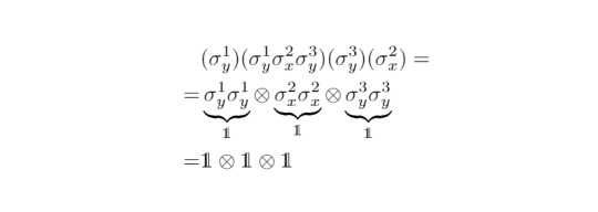
Thinking about noncontextual values would make it reasonable to assign the value 1⋅1⋅1=1 to the measurement corresponding to this product of operators [There are actually more mathematical details to this step, but for simplicity I will omit them and rely on the intuition]. Doing the same with the horizontal line yields

The assignment of a noncontextual value to the measurement corresponding to this whole operator would be 1⋅(-1)⋅1=-1. All in all this would mean that one could assign to the product of all 10 operators the value 1⋅1⋅1⋅1⋅(-1)=-1. But on the other hand any of the 10 operators of the pentagram is at the intersection of two lines, therefore each of them appears twice in the whole product of all lines. Then, no matter whether one assigns +1 or -1 to each of the operators, since they appear twice, their joint product will be +1. With this, we arrived at the contradiction +1=-1. Therefore it is not possible to assign noncontextual pre-measurement values to arbitrary sets of operators (i.e. observables) in quantum mechanics.

Again I'd like to emphasize that this proof does not directly address the issue of (non)locality as it was the case here. We do not refer to a particular state or specific spatiotemporal experimental setup - it's in a sense more general. This can be neatly summarized in Mermin's words:

"This new version [2] of Bell’s Theorem makes it clear that the use of a particular state is required to provide the information that is lost when one permits the assignment of non-contextual values only when non-contextuality is a consequence of locality." - David Mermin p.20 [1]

---

[1] Mermin - Hidden Variables and the Two Theorems of John Bell, arXiv:1802.10119, p.17

[2] Mermin - What's wrong with these elements of reality, https://doi.org/10.1063/1.2810588

[3] Leifer - Is the quantum state real?, arXiv:1409.1570 (See Def. C.1, C.2)

[dat-physics-gal]

Btw as someone who is literally watching a quantum mechanics lecture right now, I am upset. (Ok technically it’s a higher analysis lecture about operators on Hilbertspaces, but you get my point.)

(observes you)

[eatsleepmath]

Hilbert spaces, 1:

I’ve been reading Pedersen’s Analysis Now for a model-theoretic functional analysis reading course this term. We’re starting the section on Hilbert spaces (and the theory of operators on Hilbert spaces) and it’s my turn to present, so I’ve written some notes that I’ll also post here.

Definition. A sesquilinear form on a vector space \(X\) is a map \[( \cdot | \cdot) : X \times X \to \mathbb{F}\] which is linear in the first variable and conjugate linear in the second. To be precise, it’s additive in either variable, but compatible/\(\mathbb{F}\)-equivariant up to conjugation in the second variable.

Definition. To each sesquilinear form \((\cdot | \cdot)\) we define the adjoint form \(( \cdot | \cdot )^*\) by \[(x | y)^* \overset{\operatorname{df}}{=} \overline{(y | x)},\] for all \(x\) and \(y\) in \(X\). We say that the form is self-adjoint if it is its own adjoint. (When \(\mathbb{F} = \mathbb{R},\) the term symmetric is used.)

Claim. When \(\mathbb{F}\) is \(\mathbb{C},\) a calculation (or simply observing that \(S^1\) acts via isometries) shows that \[4(x | y) = \sum_{k = 0}^3 i^k(x + i^k y | x + i^k y).\]

Proof. Expanding the sum gives \[(x | x) + (y | x) + (x | y) + (y | y)\]\[+ i(x | x) + i(x|iy) + i(iy|x) + i(iy|iy)\]\[- (x|x) - (x|-y) - (-y|x) - (-y | -y)\]\[ -i (x | x) - i(x | -iy) - i(-iy | x) - i(-iy|-iy)\] \[= (x|x)(1 + i - 1 - i) + (y | x)(1 - 1 + 1 - 1)\]\[ + (x|y)(1 + 1 + 1 + 1) + (y|y)(1 -i^3 - 1 + i^3)\]\[= 4(x|y).\] \(\square\)

We say a sesquilinear form \(( \cdot | \cdot)\) is positive if \((x|x) \geq 0\) for every \(x \in X\); thus, for \(\mathbb{F} = \mathbb{C}\) a positive form is automatically self-adjoint, since the above claim shows (after a nearly-identical calculation) that a sesquilinear form is self-adjoint if and only if \((x | x) \in \mathbb{R}\) for every \(x \in X\).

On a real space, a positive form might not be symmetric. For example, take a nontrivial quadratic form.

Definition. An inner product on \(X\) is a positive, self-adjoint sesquilinear form such that \((x | x) = 0\) implies \(x = 0\) for all \(x \in X\), i.e. the form is positive-definite in addition to being positive.

Definition. From similar computations from the claim above, we obtain the following polarization identities: in \(\mathbb{C},\) \[4(x|y) = \sum_{k=0}^3 i^k || x + i^k y||^2,\] and in \(\mathbb{R}\), \[4(x|y) = || x + y||^2 - ||x - y||^2.\]

Lemma. (Cauchy-Schwarz inequality) Let \(\alpha\) be a scalar in \(\mathbb{F}\). The formula \[|\alpha|^2 ||x||^2 + 2 \Re \alpha(x | y) + ||y||^2 = ||\alpha x + y||^2 \geq 0\] for \(x\) and \(y\) in \(X\) immediately leads to the Cauchy-Schwarz inequality: \[|(x|y)| \leq ||x|| ||y||.\]

Inserting this into the above formula, it follows that the norm function \(|| \cdot ||\) is subadditive, and therefore a seminorm on \(X\). In the case when \(( \cdot | \cdot)\) is an inner product, the homogeneous function \(||x|| \overset{\operatorname{df}}{=} (x | x)^{½}\) is a norm, and equality holds in the Cauchy-Schwarz inequality if and only if \(x\) and \(y\) are scalar multiples of each other.

Lemma. Elementary computations show that the norm arising from an inner product space satisfies the parallelogram law, namely \[||x+y||^2 + ||x - y||^2 = 2(||x||^2 + ||y||^2).\]

Conversely, one way verify that if a norm satisfies the parallelogram law, then the polarization identities from before induce inner products on \(X\) (which one depending, of course, on the ground field.)

Definition. A Hilbert space is a vector space \(\mathfrak{H}\) with an inner product \(( \cdot | \cdot )\), such that \(\mathfrak{H}\) is a Banach space with respect to the associated norm.

Examples. - The Euclidean spaces are Hilbert spaces.

- The spaces of compactly-supported continuous functions on Euclidean spaces are a Hilbert space with inner product given by \((f | g ) \overset{\operatorname{df}}{=} \int f \overline{g} dx;\) the associated norm is the \(2\)-norm, and after completing we get the Hilbert space \(L^2 \mathbb{R}\). 

(More generally, you could replace the Lebesgue integral above with a Radon integral on a locally compact Hausdorff space and the same construction gives you a Hilbert space \(L^2 X.\))

Algebraic direct sums iare formed as in \(\mathbf{Ban}\), with the new inner product being defined pointwise.

Lemma. If \(\mathbf{C}\) is a closed nonempty convex subset of a Hilbert space \(\mathfrak{H}\), there is for each \(y\) in \(\mathfrak{H}\) a unique \(x\) in \(\mathfrak{C}\) that minimizes the distance from \(y\) to \(\mathfrak{C}\).

Proof. By translation variance, we can assume \(y = 0\). Let \(\alpha\) be the infimum of the norms of elements in \(\mathfrak{C}\). Choose a sequence \((x_n)\) from \(\mathfrak{C}\) witnessing this.

For any \(y\) and \(z\) in \(\mathfrak{C}\), the parallelogram law (and convexity, whence \(½(y+z) \in \mathfrak{C}\)) gives \[2 \left( ||y||^2 + ||z||^2\right) = ||y+z||^2 \geq 4 \alpha^2 + ||y - z||^2,\] Hence, when \(y = x_n\) and \(z = x_m\), \((x_n)\) is a Cauchy sequence, so by completeness of a Hilbertspace there is a limit \(x\) with \(||x|| = \alpha\).

Furthermore, since the topology is Hausdorff, the limit is unique. \(\square\)

Theorem. For a closed subspace \(X\) of a Hilbert space \(\mathfrak{H}\), let \(X^{\perp}\) be the subspace of all elements orthogonal to all of \(X\). Then each vector \(y \in \mathfrak{H}\) has a unique decomposition \(y = x + x^{\perp}\), and \(x\) and \(x^{\perp}\) are the nearest points in \(X\) and \(X^{\perp}\) to \(y\); furthermore \(\mathfrak{H} = X \oplus X^{\perp}\) and \(\left(X^{\perp}\right)^{\perp} = X.\)

Proof. More or less automatic verification.

Given \(y\) in \(\mathfrak{H}\) we take \(x\) to be the nearest point in \(X\) to \(y\) gotten by the previous lemma; put \(x^{\perp}\) to be \(y - x\). For every \(z \in X\) and \(\epsilon > 0\),

\[||x^{\perp}||^2 = ||y - x||^2 \leq ||y - (x + \epsilon z)||^2\]

\[= ||x^{\perp} - \epsilon z||^2 = ||x^{\perp}||^2 - 2 \epsilon \Re(x^{\perp}|z) + \epsilon^2||z||^2.\]

It follows that \(2 \Re(x^{\perp}|z) \leq \epsilon ||z||^2\) for every \(\epsilon > 0\), whence \(\Re(x^{\perp}|z) \leq 0\) for every \(z\). Since \(X\) is a linear subspace, this implies that \((x^{\perp}|z)\) is zero, so that \(x^{\perp}\) deserves its name and is in \(X^{\perp}\). \(\square\)

Corollary. For every subset \(X \subset \mathfrak{H}\), the smallest closed subspace of \(\mathfrak{H}\) containing \(X\) is \(X\)-double perp. In particular, if \(X\) is a subspace of \(\mathfrak{H}\), then \(\overline{X}\) is \(X\)-double perp.

Proposition. The maps \(\Phi \overset{\operatorname{df}}{=} ( \cdot | x )\) are conjugate linear isometries of \(\mathfrak{H}\) onto \(\mathfrak{H}^*\).

Proof. Tautologically conjugate-linear; \(\Phi\) is maximized by CZ-inequality on \(x/||x||\) on the unit ball, so the norm of \(\Phi\) is precisely \(||x||\). \(\square\)

Remark. Take \(\varphi\) in \(\mathfrak{H}^* \backslash \{0\}\), and put \(X = \ker \varphi\). Since \(X\) is a proper closed subspace of \(\mathfrak{H}\), there is a vector \(x \in X^{\perp}\) such that \(\varphi(x) = 1.\) For every \(y \in \mathfrak{H}\), we see that \(y - \varphi(y) x \in X\), hence \[(y | x) = (y - \varphi(y) x + \varphi(y) x | x) = \varphi(y) ||x||^2.\] It follows that \(\varphi = \Phi(||x||^{-2} x).\)

Definition. We define the weak topology on a Hilbert space \(\mathfrak{H}\) as the initial topology corresponding to the family of functionals \(x \mapsto (x | y),\) so essentially the weak topology it induces…on itself. Since it is isometric with its dual, the weak topology on \(\mathfrak{H}\) is the weak-star topology on \(\mathfrak{H}^*\) pulled back via the isometry, and the unit ball in \(\mathfrak{H}\) is weakly compact.

We’ll see that every operator in \(\mathbf{B}(\mathfrak{H})\) is continuous as a function \(\mathfrak{H} \to \mathfrak{H}\) when both copies have the weak topology; we say that \(T\) is weak-weak continuous.

Conversely, if \(T\) is a weak-weak cts operator, we can invoke the closed graph theorem to see that \(T \in \mathbf{B}(\mathfrak{H})\). Indeed, if \(x_n \to x\) and \(T x_n \to y\) in the norm topology, then \(x_n \to x\) and \(T x_n \to y\) weakly since the norm topology refines the weak topology; by assumption \(T x_n \to Tx\) weakly, whence \(Tx = y,\) as was required.

Similarly, every norm-weak continuous operator on \(\mathfrak{H}\) is bounded. We’ll see later operator that is weak-norm continuous must have finite rank, which is neat; we’ll later also modify this to give a characterization of the compact operators (which are a good candidate for treating infinitesimal elements.)

[losbraensos]

Spin-Pauli-Matrices They seem so trivial but everytime I revisit them I understand another aspect of them. I invite everyone to transform some spin basis with me, 2dim. Hilbertspaces are a safespace for my ❤.

[govindhtech]

Hilbert Space & Qubits: finding the Power of Quantum States

Space Hilbert

Science Corrects Qudits' Quantum Errors for the First Time

Yale researchers made fault-tolerant quantum computing breakthroughs. The scientists demonstrated the first experimental quantum error correction (QEC) for higher-dimensional qudits, according to Nature. This is needed to overcome quantum information's error-prone and noisy fragility.

The Hilbert space dimension is fundamental to quantum computing. This dimension indicates how many quantum states a quantum computer may access. A larger Hilbert space is valued for its ability to support more complex quantum operations and quantum error correction. Traditional classical computers use bits that can only be 0 or 1. Most quantum computers use qubits. Qubits have up (1) and down (0) states like classical bits. Quantum superposition allows qubits to be in both states, which is important. Qubit Hilbert space is two-dimensional complex vector space.

The Yale study examines qudits, quantum systems that store quantum information and can exist in multiple states. Scientific interest in qudits over qubits is rising because to the assumption that “bigger is better” in Hilbert space. Qudits simplify complex quantum computer construction tasks. These include building quantum gates, running complex algorithms, creating “magic” states for quantum computers, and better simulating complex quantum systems than qubits. Researchers are studying qudit-based quantum computers using photons, ultracold atoms and molecules, and superconducting circuits.

Despite their theoretical merits, qubits have been the only focus of quantum error correction experiments, supporting real-world QEC demonstrations. The Yale paper deviates from this trend by providing the first experimental proof of error correction for two types of qudits: a three-level qutrit and a four-level ququart.

The researchers used the Gottesman Kitaev Preskill (GKP) bosonic code for this landmark demonstration. This code is suitable for encoding quantum information in continuous variables of bosonic systems like light or microwave photons due to its hardware efficiency. The researchers optimised the qutrit and ququart systems for ternary (3-level) and quaternary (4-level) quantum memory using reinforcement learning. This machine learning employs trial and error to determine the optimum methods for running quantum gates or fixing mistakes.

The experiment exceeded error correction's break-even. This is a turning moment in QEC, proving that error correction is reducing errors rather than introducing them. The researchers created a more realistic and hardware-efficient QEC approach by directly using qudits' higher Hilbert space dimension.

GKP qudit states may have a trade-off, researchers discovered. Logical qudits have higher photon loss and dephasing rates than other techniques, which may limit the longevity of quantum information in them. This potential drawback is outweighed by the benefit of having more logical quantum states in a single physical system.

These results are a huge step towards scalable and dependable quantum computers, as described in the Nature study “Quantum error correction of qudits beyond break-even”. Successful qudit QEC demonstration has great potential. This breakthrough could advance medicine, materials, and encryption.