#composite micrograph

[sitting-on-me-bum]

A recent study in Nature Communications suggests that by 24 months, signs of heightened immune activity in most long-COVID patients will have returned to normal levels. Pictured above is a composite colored scanning electron micrograph of immune cells—including a single macrophage, two dendritic cells, and numerous white blood cells—involved in a cytokine storm, a life-threatening immune disorder. Cytokines are important for normal immune response, but when too many are released simultaneously it can be harmful.

COMPOSITE MICROGRAPH BY STEVE GSCHMEISSNER, SCIENCE PHOTO LIBRARY

[materialsscienceandengineering]

Fe, C 0.4, Mn 0.8 (wt%) steel, normalised

Processing Normalised 800 ºC [...] Sample preparation Nital Technique Reflected light microscopy Length bar 400 μm / 100 µm Further information A hypoeutectoid alloy (carbon composition less than eutectoid). The first phase formed upon cooling from the austenite phase field is proeutectoid ferrite. Due to the lower solubility of carbon in ferrite, carbon is partitioned into the remaining austenite. At the eutectoid point the remaining carbon enriched austenite transforms to pearlite (a mixture of ferrite and cementite) which is the darker region of the micrograph. The proportion of pearlite is dependent upon the overall composition. The ferrite (light areas) is a good example of an allotriomorphic ferrite. This means that its shape does not reflect its internal crystalline symmetry as it nucleates on the austenite grain boundaries and hence follows the shape of the boundaries, the remaining austenite within the ferrite then transforms to pearlite, and is surrounded by the ferrite. Contributor Dr R F Cochrane Organisation Department of Materials, University of Leeds

Sources: ( 1 ) ( 2 )

[estera-shirin]

Shviti, Jerusalem, Palestine/Eretz Israel, 1900 CE

This shviti was created by Monsohn, A. L.

According to the museum: "An early stone lithograph shiviti combining Kabbalistic elements from Sefer Yitzirah with the Shiviti. The composition is done in micrographic writing, including a highly stylized rendition of the Menorah with the 67th Psalm. The sheet is a "minchah Sheluchah" page, meant to be presented as a gift from the person who ordered the publishing of this sheet to one of his friends."

[mybeingthere]

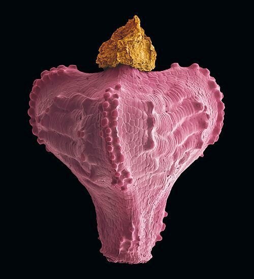
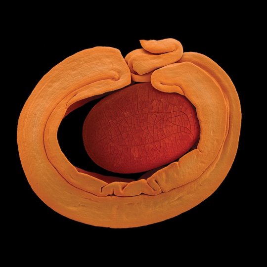
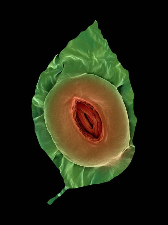
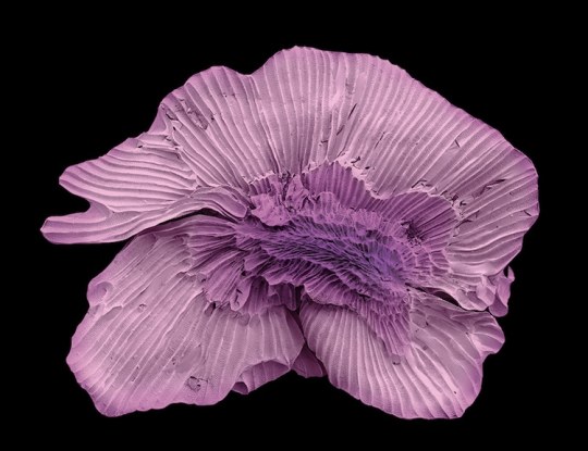
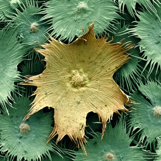
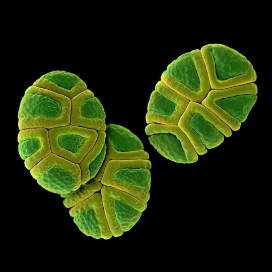
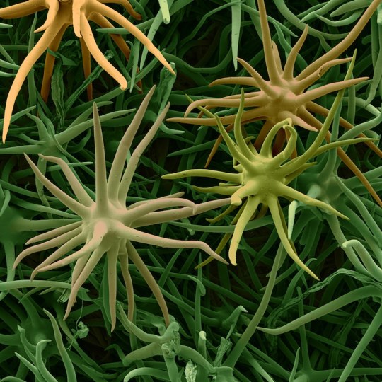
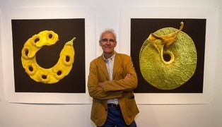
Rob Kesseler is a visual artist and Emeritus Professor of Arts, Design & Science at Central Saint Martins, London. For the past twenty years he has worked with botanical scientists and molecular biologists around the world to explore the living world at a microscopic level. Using a range of complex microscopy processes he creates multi-frame composite images of plant organs.

Using scanning electron microscopy and a mix of microscopic, scientific, digital, and manual processes, artist Rob Kesseler develops coloured micrographs of the intricate patterns within pollen and seed grains, plant cells, and leaf structures. The photographs feature specifics of cellular composition that are undetectable without magnification.

Kesseler tells that as a child, his father gifted him a microscope, marking a pivotal moment in his creative career. “What the microscope gave me was an unprecedented view of nature, a second vision,” he writes, “and awareness that there existed another world of forms, colours and patterns beyond what I could normally see.” The artist says his use of color is inspired by the time he spends researching and observing, and that just like nature, he employs it to attract attention.

[dapurinthos]

This volume, the third in a series describing the history, characteristics, and scientific analysis of artists’ pigments, covers 10 pigments, from some of the earliest man-made colorants, such as Egyptian blue and gamboge, to the 20th century’s titanium dioxide whites. Also included are orpiment and realgar; indigo and woad; madder and alizarin; Vandyke brown; Prussian blue; emerald green and Scheele’s green; and chromium oxide greens. More than 200 images depict artworks created with the pigments described, as well as x-ray diffraction patterns, scanning electron micrographs, and thin-layer chromatographs. The chapters provide details on nomenclature and general composition; history of use; color, permanence, compatibility, and painting and handling qualities; composition; characterization and identification through technical methods and procedures; and notable instances of use by a particular artist or in a specific work.

now i will have actual samples of scheele's green and paris green to colour match at the paint store!

[mirrrraaa]

Ship Tank Cleaning

Ship Tank Cleaning

MASTER GUIDE: CRUDE OIL STORAGE TANK CLEANING – THE DEFINITIVE RESOURCE

I. Advanced Sludge Characterization

1.1 Petrochemical Analysis

SARA Fractions (Saturates/Aromatics/Resins/Asphaltenes):

Typical Distribution in Sludge:

math

\text{Asphaltenes} = 15-25\%,\ \text{Resins} = 20-35\%

Rheological Properties:

Yield Stress: 50-200 Pa (measured with viscometers)

Thixotropy Index: 1.5-3.0

1.2 Microstructural Imaging

SEM-EDS Analysis:

Fig. 1: SEM micrograph showing asphaltene aggregates (10μm scale)

Table: EDS elemental composition (weight %)

Element  Fresh Crude    Aged Sludge

Carbon    82-85%  76-78%

Sulfur      1-2%      3-5%

Vanadium       <50 ppm 300-500 ppm

II. Cutting-Edge Cleaning Technologies

2.1 High-Definition Hydroblasting

3D Nozzle Trajectory Optimization:

CFD-modeled spray patterns (Fig. 2)

Optimal parameters:

Pressure: 280-350 bar

Nozzle angle: 15-25°

Coverage rate: 8-12 m²/min

2.2 Plasma Arc Cleaning

Technical Specifications:

Power: 40-60 kW DC

Temperature: 8,000-12,000°C (localized)

Effectiveness: 99.9% hydrocarbon removal

2.3 Nanoremediation

Magnetic Nanoparticles:

Fe₃O₄ core with oleophilic coating

Recovery rate: 92% at 0.5 g/L concentration

III. Operational Excellence Framework

3.1 Decision Matrix for Method Selection

Ship Tank Cleaning

Criteria    Weight    Robotic   Chemical Thermal

Safety     30% 9     6     7

Cost Efficiency 25% 7     8     5

Environmental       20% 8     5     6

Speed     15% 9     7     8

Flexibility 10% 6     9     5

*Scoring: 1-10 (10=best)*

3.2 Gantt Chart for Turnaround

Diagram

Code

IV. HSE Protocols Redefined

4.1 Quantified Risk Assessment (QRA)

Fault Tree Analysis:

Probability of H₂S exposure:

math

P_{total} = P_1 \times P_2 = 0.2 \times 0.05 = 0.01 (1\%)

Where:

P₁ = Probability of gas detection failure

P₂ = Probability of PPE breach

4.2 Emergency Response Drills

Scenario Training Modules

Confined space rescue (5-minute response)

Foam suppression system activation

Medical evacuation procedures

V. Economic Modeling

5.1 Total Cost of Ownership (TCO)

math

TCO = C_{capex} + \sum_{n=1}^{5} \frac{C_{opex}}{(1+r)^n} + C_{downtime}

Case Example:

Robotic system: $2.1M over 5 years (15% IRR)

Manual cleaning: $3.4M over 5 years (9% IRR)

5.2 Carbon Credit Potential

CO₂ Equivalent Savings:

Automated vs manual: 120 tons CO₂e per cleaning

Monetization: $6,000 at $50/ton (EU ETS price)

VI. Digital Transformation

6.1 AI-Powered Predictive Cleaning

Machine Learning Model:

Input parameters:

Crude TAN (Total Acid Number)

BS&W history

Temperature fluctuations

Output: Optimal cleaning interval (accuracy: ±3 days)

6.2 Blockchain Documentation

Smart Contract Features:

Automated regulatory reporting

Waste tracking with RFID tags

Immutable safety inspection logs

VII. Global Regulatory Atlas

7.1 Comparative Matrix

Requirement  USA (OSHA)    EU (ATEX)       UAE (ADNOC)

Entry permits  1910.146       137-2013       COP 48.01

H₂S monitoring       10 ppm TWA  5 ppm STEL    2 ppm alarm

Waste classification D001       HP7 Class 2.1

VIII. Expert Interviews

8.1 Q&A with Shell's Tank Integrity Manager

Key Insight:

*"Our new laser ablation system reduced cleaning downtime by 40%, but the real breakthrough was integrating real-time viscosity sensors with our ERP system."*

8.2 MIT Energy Initiative Findings

Research Paper:

*"Nanoparticle-enhanced solvents demonstrated 30% higher recovery rates in heavy crude applications (Journal of Petroleum Tech, 2023)."*

IX. Implementation Toolkit

9.1 Field Operations Manual

Checklist Templates:

Pre-entry verification (30-point list)

Waste manifest (API 13.1 compliant)

PPE inspection log

9.2 Calculation Worksheets

Sludge Volume Estimator:

math

V_{sludge} = \pi r^2 \times h_{avg} \times \rho_{compact}

Ventilation Calculator:

math

Q = \frac{V \times ACH}{60}

X. Future Outlook (2025-2030)

Autonomous Cleaning Drones (Under development by Aramco)

Supercritical CO₂ Extraction (Pilot phase in Norway)

Self-Healing Tank Linings (Graphene nanocomposite trials)

[miiirrrooohhh]

Ship Tank Cleaning

Ship Tank Cleaning

MASTER GUIDE: CRUDE OIL STORAGE TANK CLEANING – THE DEFINITIVE RESOURCE

I. Advanced Sludge Characterization

1.1 Petrochemical Analysis

SARA Fractions (Saturates/Aromatics/Resins/Asphaltenes):

Typical Distribution in Sludge:

math

\text{Asphaltenes} = 15-25\%,\ \text{Resins} = 20-35\%

Rheological Properties:

Yield Stress: 50-200 Pa (measured with viscometers)

Thixotropy Index: 1.5-3.0

1.2 Microstructural Imaging

SEM-EDS Analysis:

Fig. 1: SEM micrograph showing asphaltene aggregates (10μm scale)

Table: EDS elemental composition (weight %)

Element  Fresh Crude    Aged Sludge

Carbon    82-85%  76-78%

Sulfur      1-2%      3-5%

Vanadium       <50 ppm 300-500 ppm

II. Cutting-Edge Cleaning Technologies

2.1 High-Definition Hydroblasting

3D Nozzle Trajectory Optimization:

CFD-modeled spray patterns (Fig. 2)

Optimal parameters:

Pressure: 280-350 bar

Nozzle angle: 15-25°

Coverage rate: 8-12 m²/min

2.2 Plasma Arc Cleaning

Technical Specifications:

Power: 40-60 kW DC

Temperature: 8,000-12,000°C (localized)

Effectiveness: 99.9% hydrocarbon removal

2.3 Nanoremediation

Magnetic Nanoparticles:

Fe₃O₄ core with oleophilic coating

Recovery rate: 92% at 0.5 g/L concentration

III. Operational Excellence Framework

3.1 Decision Matrix for Method Selection

Ship Tank Cleaning

Criteria    Weight    Robotic   Chemical Thermal

Safety     30% 9     6     7

Cost Efficiency 25% 7     8     5

Environmental       20% 8     5     6

Speed     15% 9     7     8

Flexibility 10% 6     9     5

*Scoring: 1-10 (10=best)*

3.2 Gantt Chart for Turnaround

Diagram

Code

IV. HSE Protocols Redefined

4.1 Quantified Risk Assessment (QRA)

Fault Tree Analysis:

Probability of H₂S exposure:

math

P_{total} = P_1 \times P_2 = 0.2 \times 0.05 = 0.01 (1\%)

Where:

P₁ = Probability of gas detection failure

P₂ = Probability of PPE breach

4.2 Emergency Response Drills

Scenario Training Modules

Confined space rescue (5-minute response)

Foam suppression system activation

Medical evacuation procedures

V. Economic Modeling

5.1 Total Cost of Ownership (TCO)

math

TCO = C_{capex} + \sum_{n=1}^{5} \frac{C_{opex}}{(1+r)^n} + C_{downtime}

Case Example:

Robotic system: $2.1M over 5 years (15% IRR)

Manual cleaning: $3.4M over 5 years (9% IRR)

5.2 Carbon Credit Potential

CO₂ Equivalent Savings:

Automated vs manual: 120 tons CO₂e per cleaning

Monetization: $6,000 at $50/ton (EU ETS price)

VI. Digital Transformation

6.1 AI-Powered Predictive Cleaning

Machine Learning Model:

Input parameters:

Crude TAN (Total Acid Number)

BS&W history

Temperature fluctuations

Output: Optimal cleaning interval (accuracy: ±3 days)

6.2 Blockchain Documentation

Smart Contract Features:

Automated regulatory reporting

Waste tracking with RFID tags

Immutable safety inspection logs

VII. Global Regulatory Atlas

7.1 Comparative Matrix

Requirement  USA (OSHA)    EU (ATEX)       UAE (ADNOC)

Entry permits  1910.146       137-2013       COP 48.01

H₂S monitoring       10 ppm TWA  5 ppm STEL    2 ppm alarm

Waste classification D001       HP7 Class 2.1

VIII. Expert Interviews

8.1 Q&A with Shell's Tank Integrity Manager

Key Insight:

*"Our new laser ablation system reduced cleaning downtime by 40%, but the real breakthrough was integrating real-time viscosity sensors with our ERP system."*

8.2 MIT Energy Initiative Findings

Research Paper:

*"Nanoparticle-enhanced solvents demonstrated 30% higher recovery rates in heavy crude applications (Journal of Petroleum Tech, 2023)."*

IX. Implementation Toolkit

9.1 Field Operations Manual

Checklist Templates:

Pre-entry verification (30-point list)

Waste manifest (API 13.1 compliant)

PPE inspection log

9.2 Calculation Worksheets

Sludge Volume Estimator:

math

V_{sludge} = \pi r^2 \times h_{avg} \times \rho_{compact}

Ventilation Calculator:

math

Q = \frac{V \times ACH}{60}

X. Future Outlook (2025-2030)

Autonomous Cleaning Drones (Under development by Aramco)

Supercritical CO₂ Extraction (Pilot phase in Norway)

Self-Healing Tank Linings (Graphene nanocomposite trials)

[aliiiitotoo]

Ship Tank Cleaning

Ship Tank Cleaning

MASTER GUIDE: CRUDE OIL STORAGE TANK CLEANING – THE DEFINITIVE RESOURCE

I. Advanced Sludge Characterization

1.1 Petrochemical Analysis

SARA Fractions (Saturates/Aromatics/Resins/Asphaltenes):

Typical Distribution in Sludge:

math

\text{Asphaltenes} = 15-25\%,\ \text{Resins} = 20-35\%

Rheological Properties:

Yield Stress: 50-200 Pa (measured with viscometers)

Thixotropy Index: 1.5-3.0

1.2 Microstructural Imaging

SEM-EDS Analysis:

Fig. 1: SEM micrograph showing asphaltene aggregates (10μm scale)

Table: EDS elemental composition (weight %)

Element  Fresh Crude    Aged Sludge

Carbon    82-85%  76-78%

Sulfur      1-2%      3-5%

Vanadium       <50 ppm 300-500 ppm

II. Cutting-Edge Cleaning Technologies

2.1 High-Definition Hydroblasting

3D Nozzle Trajectory Optimization:

CFD-modeled spray patterns (Fig. 2)

Optimal parameters:

Pressure: 280-350 bar

Nozzle angle: 15-25°

Coverage rate: 8-12 m²/min

2.2 Plasma Arc Cleaning

Technical Specifications:

Power: 40-60 kW DC

Temperature: 8,000-12,000°C (localized)

Effectiveness: 99.9% hydrocarbon removal

2.3 Nanoremediation

Magnetic Nanoparticles:

Fe₃O₄ core with oleophilic coating

Recovery rate: 92% at 0.5 g/L concentration

III. Operational Excellence Framework

3.1 Decision Matrix for Method Selection

Ship Tank Cleaning

Criteria    Weight    Robotic   Chemical Thermal

Safety     30% 9     6     7

Cost Efficiency 25% 7     8     5

Environmental       20% 8     5     6

Speed     15% 9     7     8

Flexibility 10% 6     9     5

*Scoring: 1-10 (10=best)*

3.2 Gantt Chart for Turnaround

Diagram

Code

IV. HSE Protocols Redefined

4.1 Quantified Risk Assessment (QRA)

Fault Tree Analysis:

Probability of H₂S exposure:

math

P_{total} = P_1 \times P_2 = 0.2 \times 0.05 = 0.01 (1\%)

Where:

P₁ = Probability of gas detection failure

P₂ = Probability of PPE breach

4.2 Emergency Response Drills

Scenario Training Modules

Confined space rescue (5-minute response)

Foam suppression system activation

Medical evacuation procedures

V. Economic Modeling

5.1 Total Cost of Ownership (TCO)

math

TCO = C_{capex} + \sum_{n=1}^{5} \frac{C_{opex}}{(1+r)^n} + C_{downtime}

Case Example:

Robotic system: $2.1M over 5 years (15% IRR)

Manual cleaning: $3.4M over 5 years (9% IRR)

5.2 Carbon Credit Potential

CO₂ Equivalent Savings:

Automated vs manual: 120 tons CO₂e per cleaning

Monetization: $6,000 at $50/ton (EU ETS price)

VI. Digital Transformation

6.1 AI-Powered Predictive Cleaning

Machine Learning Model:

Input parameters:

Crude TAN (Total Acid Number)

BS&W history

Temperature fluctuations

Output: Optimal cleaning interval (accuracy: ±3 days)

6.2 Blockchain Documentation

Smart Contract Features:

Automated regulatory reporting

Waste tracking with RFID tags

Immutable safety inspection logs

VII. Global Regulatory Atlas

7.1 Comparative Matrix

Requirement  USA (OSHA)    EU (ATEX)       UAE (ADNOC)

Entry permits  1910.146       137-2013       COP 48.01

H₂S monitoring       10 ppm TWA  5 ppm STEL    2 ppm alarm

Waste classification D001       HP7 Class 2.1

VIII. Expert Interviews

8.1 Q&A with Shell's Tank Integrity Manager

Key Insight:

*"Our new laser ablation system reduced cleaning downtime by 40%, but the real breakthrough was integrating real-time viscosity sensors with our ERP system."*

8.2 MIT Energy Initiative Findings

Research Paper:

*"Nanoparticle-enhanced solvents demonstrated 30% higher recovery rates in heavy crude applications (Journal of Petroleum Tech, 2023)."*

IX. Implementation Toolkit

9.1 Field Operations Manual

Checklist Templates:

Pre-entry verification (30-point list)

Waste manifest (API 13.1 compliant)

PPE inspection log

9.2 Calculation Worksheets

Sludge Volume Estimator:

math

V_{sludge} = \pi r^2 \times h_{avg} \times \rho_{compact}

Ventilation Calculator:

math

Q = \frac{V \times ACH}{60}

X. Future Outlook (2025-2030)

Autonomous Cleaning Drones (Under development by Aramco)

Supercritical CO₂ Extraction (Pilot phase in Norway)

Self-Healing Tank Linings (Graphene nanocomposite trials)

[safsff]

Ship Tank Cleaning

Ship Tank Cleaning

MASTER GUIDE: CRUDE OIL STORAGE TANK CLEANING – THE DEFINITIVE RESOURCE

I. Advanced Sludge Characterization

1.1 Petrochemical Analysis

SARA Fractions (Saturates/Aromatics/Resins/Asphaltenes):

Typical Distribution in Sludge:

math

\text{Asphaltenes} = 15-25\%,\ \text{Resins} = 20-35\%

Rheological Properties:

Yield Stress: 50-200 Pa (measured with viscometers)

Thixotropy Index: 1.5-3.0

1.2 Microstructural Imaging

SEM-EDS Analysis:

Fig. 1: SEM micrograph showing asphaltene aggregates (10μm scale)

Table: EDS elemental composition (weight %)

Element  Fresh Crude    Aged Sludge

Carbon    82-85%  76-78%

Sulfur      1-2%      3-5%

Vanadium       <50 ppm 300-500 ppm

II. Cutting-Edge Cleaning Technologies

2.1 High-Definition Hydroblasting

3D Nozzle Trajectory Optimization:

CFD-modeled spray patterns (Fig. 2)

Optimal parameters:

Pressure: 280-350 bar

Nozzle angle: 15-25°

Coverage rate: 8-12 m²/min

2.2 Plasma Arc Cleaning

Technical Specifications:

Power: 40-60 kW DC

Temperature: 8,000-12,000°C (localized)

Effectiveness: 99.9% hydrocarbon removal

2.3 Nanoremediation

Magnetic Nanoparticles:

Fe₃O₄ core with oleophilic coating

Recovery rate: 92% at 0.5 g/L concentration

III. Operational Excellence Framework

3.1 Decision Matrix for Method Selection

Ship Tank Cleaning

Criteria    Weight    Robotic   Chemical Thermal

Safety     30% 9     6     7

Cost Efficiency 25% 7     8     5

Environmental       20% 8     5     6

Speed     15% 9     7     8

Flexibility 10% 6     9     5

*Scoring: 1-10 (10=best)*

3.2 Gantt Chart for Turnaround

Diagram

Code

IV. HSE Protocols Redefined

4.1 Quantified Risk Assessment (QRA)

Fault Tree Analysis:

Probability of H₂S exposure:

math

P_{total} = P_1 \times P_2 = 0.2 \times 0.05 = 0.01 (1\%)

Where:

P₁ = Probability of gas detection failure

P₂ = Probability of PPE breach

4.2 Emergency Response Drills

Scenario Training Modules

Confined space rescue (5-minute response)

Foam suppression system activation

Medical evacuation procedures

V. Economic Modeling

5.1 Total Cost of Ownership (TCO)

math

TCO = C_{capex} + \sum_{n=1}^{5} \frac{C_{opex}}{(1+r)^n} + C_{downtime}

Case Example:

Robotic system: $2.1M over 5 years (15% IRR)

Manual cleaning: $3.4M over 5 years (9% IRR)

5.2 Carbon Credit Potential

CO₂ Equivalent Savings:

Automated vs manual: 120 tons CO₂e per cleaning

Monetization: $6,000 at $50/ton (EU ETS price)

VI. Digital Transformation

6.1 AI-Powered Predictive Cleaning

Machine Learning Model:

Input parameters:

Crude TAN (Total Acid Number)

BS&W history

Temperature fluctuations

Output: Optimal cleaning interval (accuracy: ±3 days)

6.2 Blockchain Documentation

Smart Contract Features:

Automated regulatory reporting

Waste tracking with RFID tags

Immutable safety inspection logs

VII. Global Regulatory Atlas

7.1 Comparative Matrix

Requirement  USA (OSHA)    EU (ATEX)       UAE (ADNOC)

Entry permits  1910.146       137-2013       COP 48.01

H₂S monitoring       10 ppm TWA  5 ppm STEL    2 ppm alarm

Waste classification D001       HP7 Class 2.1

VIII. Expert Interviews

8.1 Q&A with Shell's Tank Integrity Manager

Key Insight:

*"Our new laser ablation system reduced cleaning downtime by 40%, but the real breakthrough was integrating real-time viscosity sensors with our ERP system."*

8.2 MIT Energy Initiative Findings

Research Paper:

*"Nanoparticle-enhanced solvents demonstrated 30% higher recovery rates in heavy crude applications (Journal of Petroleum Tech, 2023)."*

IX. Implementation Toolkit

9.1 Field Operations Manual

Checklist Templates:

Pre-entry verification (30-point list)

Waste manifest (API 13.1 compliant)

PPE inspection log

9.2 Calculation Worksheets

Sludge Volume Estimator:

math

V_{sludge} = \pi r^2 \times h_{avg} \times \rho_{compact}

Ventilation Calculator:

math

Q = \frac{V \times ACH}{60}

X. Future Outlook (2025-2030)

Autonomous Cleaning Drones (Under development by Aramco)

Supercritical CO₂ Extraction (Pilot phase in Norway)

Self-Healing Tank Linings (Graphene nanocomposite trials)

[fayrozzaa]

Ship Tank Cleaning

Ship Tank Cleaning

MASTER GUIDE: CRUDE OIL STORAGE TANK CLEANING – THE DEFINITIVE RESOURCE

I. Advanced Sludge Characterization

1.1 Petrochemical Analysis

SARA Fractions (Saturates/Aromatics/Resins/Asphaltenes):

Typical Distribution in Sludge:

math

\text{Asphaltenes} = 15-25\%,\ \text{Resins} = 20-35\%

Rheological Properties:

Yield Stress: 50-200 Pa (measured with viscometers)

Thixotropy Index: 1.5-3.0

1.2 Microstructural Imaging

SEM-EDS Analysis:

Fig. 1: SEM micrograph showing asphaltene aggregates (10μm scale)

Table: EDS elemental composition (weight %)

Element  Fresh Crude    Aged Sludge

Carbon    82-85%  76-78%

Sulfur      1-2%      3-5%

Vanadium       <50 ppm 300-500 ppm

II. Cutting-Edge Cleaning Technologies

2.1 High-Definition Hydroblasting

3D Nozzle Trajectory Optimization:

CFD-modeled spray patterns (Fig. 2)

Optimal parameters:

Pressure: 280-350 bar

Nozzle angle: 15-25°

Coverage rate: 8-12 m²/min

2.2 Plasma Arc Cleaning

Technical Specifications:

Power: 40-60 kW DC

Temperature: 8,000-12,000°C (localized)

Effectiveness: 99.9% hydrocarbon removal

2.3 Nanoremediation

Magnetic Nanoparticles:

Fe₃O₄ core with oleophilic coating

Recovery rate: 92% at 0.5 g/L concentration

III. Operational Excellence Framework

3.1 Decision Matrix for Method Selection

Ship Tank Cleaning

Criteria    Weight    Robotic   Chemical Thermal

Safety     30% 9     6     7

Cost Efficiency 25% 7     8     5

Environmental       20% 8     5     6

Speed     15% 9     7     8

Flexibility 10% 6     9     5

*Scoring: 1-10 (10=best)*

3.2 Gantt Chart for Turnaround

Diagram

Code

IV. HSE Protocols Redefined

4.1 Quantified Risk Assessment (QRA)

Fault Tree Analysis:

Probability of H₂S exposure:

math

P_{total} = P_1 \times P_2 = 0.2 \times 0.05 = 0.01 (1\%)

Where:

P₁ = Probability of gas detection failure

P₂ = Probability of PPE breach

4.2 Emergency Response Drills

Scenario Training Modules

Confined space rescue (5-minute response)

Foam suppression system activation

Medical evacuation procedures

V. Economic Modeling

5.1 Total Cost of Ownership (TCO)

math

TCO = C_{capex} + \sum_{n=1}^{5} \frac{C_{opex}}{(1+r)^n} + C_{downtime}

Case Example:

Robotic system: $2.1M over 5 years (15% IRR)

Manual cleaning: $3.4M over 5 years (9% IRR)

5.2 Carbon Credit Potential

CO₂ Equivalent Savings:

Automated vs manual: 120 tons CO₂e per cleaning

Monetization: $6,000 at $50/ton (EU ETS price)

VI. Digital Transformation

6.1 AI-Powered Predictive Cleaning

Machine Learning Model:

Input parameters:

Crude TAN (Total Acid Number)

BS&W history

Temperature fluctuations

Output: Optimal cleaning interval (accuracy: ±3 days)

6.2 Blockchain Documentation

Smart Contract Features:

Automated regulatory reporting

Waste tracking with RFID tags

Immutable safety inspection logs

VII. Global Regulatory Atlas

7.1 Comparative Matrix

Requirement  USA (OSHA)    EU (ATEX)       UAE (ADNOC)

Entry permits  1910.146       137-2013       COP 48.01

H₂S monitoring       10 ppm TWA  5 ppm STEL    2 ppm alarm

Waste classification D001       HP7 Class 2.1

VIII. Expert Interviews

8.1 Q&A with Shell's Tank Integrity Manager

Key Insight:

*"Our new laser ablation system reduced cleaning downtime by 40%, but the real breakthrough was integrating real-time viscosity sensors with our ERP system."*

8.2 MIT Energy Initiative Findings

Research Paper:

*"Nanoparticle-enhanced solvents demonstrated 30% higher recovery rates in heavy crude applications (Journal of Petroleum Tech, 2023)."*

IX. Implementation Toolkit

9.1 Field Operations Manual

Checklist Templates:

Pre-entry verification (30-point list)

Waste manifest (API 13.1 compliant)

PPE inspection log

9.2 Calculation Worksheets

Sludge Volume Estimator:

math

V_{sludge} = \pi r^2 \times h_{avg} \times \rho_{compact}

Ventilation Calculator:

math

Q = \frac{V \times ACH}{60}

X. Future Outlook (2025-2030)

Autonomous Cleaning Drones (Under development by Aramco)

Supercritical CO₂ Extraction (Pilot phase in Norway)

Self-Healing Tank Linings (Graphene nanocomposite trials)

[hagooooorr]

Ship Tank Cleaning

Ship Tank Cleaning

MASTER GUIDE: CRUDE OIL STORAGE TANK CLEANING – THE DEFINITIVE RESOURCE

I. Advanced Sludge Characterization

1.1 Petrochemical Analysis

SARA Fractions (Saturates/Aromatics/Resins/Asphaltenes):

Typical Distribution in Sludge:

math

\text{Asphaltenes} = 15-25\%,\ \text{Resins} = 20-35\%

Rheological Properties:

Yield Stress: 50-200 Pa (measured with viscometers)

Thixotropy Index: 1.5-3.0

1.2 Microstructural Imaging

SEM-EDS Analysis:

Fig. 1: SEM micrograph showing asphaltene aggregates (10μm scale)

Table: EDS elemental composition (weight %)

Element  Fresh Crude    Aged Sludge

Carbon    82-85%  76-78%

Sulfur      1-2%      3-5%

Vanadium       <50 ppm 300-500 ppm

II. Cutting-Edge Cleaning Technologies

2.1 High-Definition Hydroblasting

3D Nozzle Trajectory Optimization:

CFD-modeled spray patterns (Fig. 2)

Optimal parameters:

Pressure: 280-350 bar

Nozzle angle: 15-25°

Coverage rate: 8-12 m²/min

2.2 Plasma Arc Cleaning

Technical Specifications:

Power: 40-60 kW DC

Temperature: 8,000-12,000°C (localized)

Effectiveness: 99.9% hydrocarbon removal

2.3 Nanoremediation

Magnetic Nanoparticles:

Fe₃O₄ core with oleophilic coating

Recovery rate: 92% at 0.5 g/L concentration

III. Operational Excellence Framework

3.1 Decision Matrix for Method Selection

Ship Tank Cleaning

Criteria    Weight    Robotic   Chemical Thermal

Safety     30% 9     6     7

Cost Efficiency 25% 7     8     5

Environmental       20% 8     5     6

Speed     15% 9     7     8

Flexibility 10% 6     9     5

*Scoring: 1-10 (10=best)*

3.2 Gantt Chart for Turnaround

Diagram

Code

IV. HSE Protocols Redefined

4.1 Quantified Risk Assessment (QRA)

Fault Tree Analysis:

Probability of H₂S exposure:

math

P_{total} = P_1 \times P_2 = 0.2 \times 0.05 = 0.01 (1\%)

Where:

P₁ = Probability of gas detection failure

P₂ = Probability of PPE breach

4.2 Emergency Response Drills

Scenario Training Modules

Confined space rescue (5-minute response)

Foam suppression system activation

Medical evacuation procedures

V. Economic Modeling

5.1 Total Cost of Ownership (TCO)

math

TCO = C_{capex} + \sum_{n=1}^{5} \frac{C_{opex}}{(1+r)^n} + C_{downtime}

Case Example:

Robotic system: $2.1M over 5 years (15% IRR)

Manual cleaning: $3.4M over 5 years (9% IRR)

5.2 Carbon Credit Potential

CO₂ Equivalent Savings:

Automated vs manual: 120 tons CO₂e per cleaning

Monetization: $6,000 at $50/ton (EU ETS price)

VI. Digital Transformation

6.1 AI-Powered Predictive Cleaning

Machine Learning Model:

Input parameters:

Crude TAN (Total Acid Number)

BS&W history

Temperature fluctuations

Output: Optimal cleaning interval (accuracy: ±3 days)

6.2 Blockchain Documentation

Smart Contract Features:

Automated regulatory reporting

Waste tracking with RFID tags

Immutable safety inspection logs

VII. Global Regulatory Atlas

7.1 Comparative Matrix

Requirement  USA (OSHA)    EU (ATEX)       UAE (ADNOC)

Entry permits  1910.146       137-2013       COP 48.01

H₂S monitoring       10 ppm TWA  5 ppm STEL    2 ppm alarm

Waste classification D001       HP7 Class 2.1

VIII. Expert Interviews

8.1 Q&A with Shell's Tank Integrity Manager

Key Insight:

*"Our new laser ablation system reduced cleaning downtime by 40%, but the real breakthrough was integrating real-time viscosity sensors with our ERP system."*

8.2 MIT Energy Initiative Findings

Research Paper:

*"Nanoparticle-enhanced solvents demonstrated 30% higher recovery rates in heavy crude applications (Journal of Petroleum Tech, 2023)."*

IX. Implementation Toolkit

9.1 Field Operations Manual

Checklist Templates:

Pre-entry verification (30-point list)

Waste manifest (API 13.1 compliant)

PPE inspection log

9.2 Calculation Worksheets

Sludge Volume Estimator:

math

V_{sludge} = \pi r^2 \times h_{avg} \times \rho_{compact}

Ventilation Calculator:

math

Q = \frac{V \times ACH}{60}

X. Future Outlook (2025-2030)

Autonomous Cleaning Drones (Under development by Aramco)

Supercritical CO₂ Extraction (Pilot phase in Norway)

Self-Healing Tank Linings (Graphene nanocomposite trials)

[technicalparameters]

Unveiling the Nanoscale A Comprehensive Guide to TEM Analysis in WinTech Nano

Introduction: In the realm of nanotechnology, understanding materials at the atomic and molecular levels is essential for innovation and advancement. Transmission Electron Microscopy (TEM) stands as a powerful tool, allowing researchers to delve deep into the nano world. best TEM In this blog, we'll explore the intricacies of TEM analysis, particularly in the context of WinTech Nano, and how it enables groundbreaking discoveries in various fields.

Understanding TEM: Transmission Electron Microscopy (TEM) is a microscopy technique where a beam of electrons passes through an ultra-thin specimen, interacting with the sample as it traverses. Unlike traditional light microscopes, TEM employs electrons, which have much shorter wavelengths, enabling significantly higher resolution imaging. This technique offers unparalleled insights into the structure, morphology, and composition of materials at the nanoscale.

The Role of WinTech Nano: WinTech Nano is a cutting-edge software suite designed to complement TEM analysis, providing researchers with advanced tools for data acquisition, processing, and interpretation. Its intuitive interface coupled with powerful analytical capabilities makes it a preferred choice in the nanotechnology community.

Key Features of WinTech Nano:

Image Acquisition: WinTech Nano facilitates high-resolution imaging, allowing researchers to capture detailed micrographs of their specimens. It supports various imaging modes, including bright-field, dark-field, and high-angle annular dark-field (HAADF), each offering unique insights into sample characteristics.

Spectroscopy and Elemental Analysis: With WinTech Nano, elemental analysis becomes seamless. Energy-dispersive X-ray spectroscopy (EDS) capabilities integrated into the software enable researchers to identify and quantify elemental compositions within their samples accurately.

Crystallography and Phase Analysis: Characterizing crystal structures and phases is fundamental in materials science. WinTech Nano streamlines crystallographic analysis, enabling researchers to determine lattice parameters, grain orientation, and phase distributions with precision.

In-situ Experiments: WinTech Nano supports in-situ experiments, allowing researchers to observe dynamic processes in real-time. Whether it's studying phase transformations, nanoparticle growth, or mechanical properties, WinTech Nano facilitates comprehensive data acquisition and analysis.

Applications of TEM Analysis in WinTech Nano:

Nanomaterials Synthesis: Understanding the nucleation and growth mechanisms of nanomaterials is crucial for tailoring their properties. TEM analysis in WinTech Nano aids in elucidating the morphology, size distribution, and crystal structure of synthesized nanoparticles.

Semiconductor Devices: In the semiconductor industry, precise characterization of device structures is paramount for optimizing performance. WinTech Nano enables researchers to analyze defects, interfaces, and dopant distributions in semiconductor devices with unparalleled detail.

Biological Imaging: TEM plays a pivotal role in elucidating the ultrastructure of biological specimens. With WinTech Nano, researchers can visualize cellular organelles, protein complexes, and viral particles at the nanoscale, advancing our understanding of biological processes.

Conclusion: Transmission Electron Microscopy coupled with WinTech Nano empowers researchers to explore the nanoworld with unprecedented clarity and detail. By leveraging its advanced imaging, spectroscopic, and analytical capabilities, scientists can unravel the mysteries of nanomaterials, semiconductor devices, biological systems, and beyond. As technology continues to evolve, TEM analysis in WinTech Nano will undoubtedly remain at the forefront of nanoscience research, driving innovation and discovery for years to come.read more.

[materialsscienceandengineering]

Zn coating II - Coating defects

Defect name: Zn coating Record No.: 1680 Type of defect (Internal/Surface): Surface Defect classification: Coating defects Steel name: Steel Steel composition in weight %: No data. Note:  In fact, when the micrographs of wear tracks are observed it is possible to see that the Zn-Fe surface shows more debris particles when compared to galvanized surface, Figure 1. A spread structure is visualized on the wear track of Zn-Fe surface, Figure 1d. This fact could indicate plastic deformation of the coating or wear particles compacted. Plastic deformation could take off relatively large particles by an adhesive wear mechanism. On the contrary, at the galvanized surface defined grooves were observed on the wear tracks. Some sticking of fragmented abrasive particles could also been observed, Fig 1b. These remarks are indicative that the wear mechanism predominant to galvanized surface was abrasive wear. Actually, as illustrated in Figure 1a, at the surface of the wear track formed on the Zn-Fe sample, heterogeneous spherical-like agglomerates of wear/corrosion products are observed. These products were not seen on the wear tracks of zinc, which appeared almost free of wear debris. These observations have a two-fold relevance. First the presence of the wear/corrosion products appears to be responsible for the relatively low friction coefficient monitored during the test. But, on the other hand, it indicates that the formation of wear/corrosion debris becomes quite more important in the Zn-Fe samples.

Source.

[sciencealert]

The fibrous cytoskeleton and the nucleus are stunningly highlighted in this dazzling micrograph of a embryonic mouse cell. 🐁 ​ ​Cytoskeletons help cells keep their shape but can also contract, allowing the cell to move. They also help transport substances around cells including waste, nutrients and cell organs. A cytoskeleton's composition includes actin protein filaments (green), tropomyosin protein (pink) and myosin II light chain kinase enzyme (yellow) - which helps initiate actin-myosin contractions. ​ ​📸 : @artofmicroscopy/University of Sydney

[irispublishersengineeringscience]

Global Journal of Engineering Sciences (GJES)

Investigation of the Evolution of Clay Microstructure under Different Loading Paths and Impact on Constitutive Modelling

Authored by Simona Guglielmi

The paper presents part of a research work in the field of the interpretation of the mechanical response of clays to support their constitutive modelling, according to an approach which combines the investigation of the soil element macro-behaviour, through laboratory experimental testing, with the observation of the soil features and processes at the micro-scale, through scanning electron microscopy, SEM.The effect of compression on the mechanical behaviour of clays, once reconstituted in the laboratory, has been the subject of experimental studies for many years, and has been extended to the behaviour of natural clays, which develop, in their geological history, different structure from that forming in the reconstituted during normal consolidation in the laboratory [1-3]. To date, several studies in the literature have shown that processes other than simple compression can result in an increase in the strength of clays [1-6], one example being diagenesis, which is one of those geological processes that cause an increase in stiffness and strength of the natural clay above that provided solely by the reduction in volume with compression.Diagenetic processes, which are responsible for important changes in natural clays at the microscale, typically occur at depth, under high effective stresses. They give rise to the aggradation of swelling minerals, the increase in bonding (non-frictional interparticle forces [7,8]) and changes in fabric (the arrangement of the soil particles [7,8]). As a result, natural clays can develop a structure stronger than that of the corresponding (same void ratio) reconstituted clay. This paper examines the microstructure of a natural stiff, diagenetically modified clay, by comparison with the microstructure of the same clay when reconstituted in the laboratory. This comparison is then extended to explore the evolution of microstructure after 1D compression to states preand post- gross-yield, up to large preological history is known in some detail [9]. This study is one aspect of a wider research [2,3,10-12] aimed at identifying the main physical factors and internal features which control, at the micro-scale, the material response, causing given behavioural facets. The research final aim is at assessing the influence of the different aspects of behaviour on model parameter values, hence supporting constitutive modelling and finding a relation between classes of behaviour and corresponding models and classes of clays.

Materials and Methods

Pappadai clay is a Pleistocene marine clay which was deposited in a quiet sea in the Montemesola Basin, near Taranto. The engineering geology of the clay is discussed by Cotecchia & Chandler (1995), who present paleontological and microstructural data demonstrating both the stillness of the water and the reducing conditions of the depositional environment. The main properties of the clay and its mineralogical composition are shown in Table 1.

Table 1:Index Properties and mineralogy of Pappadai clay.

The clay is of high plasticity and possesses a high carbonate content. Cotecchia & Chandler (1995) have shown that the carbonate content is largely concentrated in the sand and the silt fractions of the soil, since the carbonates increase with reducing clay fraction and plasticity index [13]. Large part of the sand and silt fractions are formed of shells of foraminifera and nannofossils. However, as will be seen, at least part of the carbonates present contribute to bonding in the clay.

Block samples were taken from a depth of 25 m during construction of a reservoir draw-off shaft and were subjected to mechanical testing [2]. The clay forming the block samples is massive and regularly laminated.

At the sampling location the clay is overconsolidated due to the erosion of some 120 m of overlying sediments. Prior to erosion the clay had undergone diagenesis resulting in a decrease in the portion of smectites, an increase in the portion of the nonswelling minerals (intergrades, Table 1), and a decrease in activity, all with respect to depth [9]. Thus, it is likely that there will have been changes in microstructure of the clay under the stress levels required to generate the mineralogical changes, that is towards the end of normal consolidation.

After unloading due to erosion, the clay in the top strata of the deposit underwent deep drying and subsequently swelled. Cotecchia e Chandler (1995) confirmed this reconstruction through the modelling of the state history of the deposit [9], the results of which are shown in Figure 1. The current profile of liquidity index against vertical effective stress at Pappadai and the modelled one are compared in Figure 1. The history of normal consolidation (stage (i)-O→P), erosion (stage (ii)-P→N), drying of the sole top strata due to lowering of the water table (stage (iii)-N→M) and water table rise (stage (iv)-M→B) was modelled and resulted in the state paths represented in the figure as continuous lines.

The last profile is “S” shaped and, as such, it is consistent with the profile of liquidity index on the undisturbed samples taken at different depth along a borehole and a shaft nearby; this latter one is the block sample B in the figure. Such undisturbed block sample is that which the experimental data presented in the following refer to. Its preconsolidation state corresponds to point P in Figure 1, as for an overconsolidation ratio (OCR) of 3.1. Such OCR resulted solely from the erosion cycle (ii) cited before, since the sample was not affected by the deep drying, which instead affected the clay layers above. For the full explanation of the reconstruction of the geological history of the clay and of the state history modelling, whose results are sketched in Figure 1, refer to [2,9].

The natural clay was reconstituted in the laboratory at a water content 1,6x liquid limit, and was one- dimensionally consolidated in a consolidometer to a vertical effective stress of 200 kPa, point A* in Figure 1, at which point it was removed from the consolidometer and placed in an oedometer where the one dimensional loading was continued. As seen in Figure 1, natural Pappadai clay followed a sedimentation compression curve (SCC; see [14] for the definition, or [1,2]) to the right of the normal consolidation line of the reconstituted clay (ICL; [1]). Thus, after a normal consolidation to point P, the natural clay already had a structure different from that of the reconstituted clay, and later underwent further changes through diagenesis.

The qualitative analysis of the clay fabric is carried out on both the natural and the reconstituted clay by means of scanning electron microscopy (SEM), using freeze-dried gold-coated clay specimens trimmed from the undisturbed block sample and from the specimens subjected to 1D compression after completion of the test and rapid undrained unloading. The microstructure of the natural clay is examined at different stages of 1D loading, i.e. at undisturbed state, soon after gross yield and to large pressures, and compared to the microstructure of the reconstituted clay after consolidation in the consolidometer and compressed to large pressures.

SEM micrographs taken on vertical fractures are shown, and sketches are reported in which fabric features are identified and local fabric arrangements are recognized. The orientation of the fabric is then quantified by means of digital image processing [15] on micrographs of size corresponding to the micro-scale representative element volume (micro-REV, [12]), recognised for the clay under study as the clay portion of size about 10-3 mm3, investigated at the medium magnification [12]. The microstructural data are related to the observed macro- response of the clay and to the constitutive hydro-mechanical parameters, highlighting what the constitutive laws deviced to represent the material macroresponse in the frame of porous media hydro-mechanics are reflecting at the micro-scale.

The bonding of Pappadai clay is such that a small undisturbed sample softens only a little after being submerged in water for several months. Drying at 120°C caused the clay to open up along the contact of the clay with silt bedding planes, and the softening of the clay on submergence was then more significant. Hence, the diagenetic bonding of Pappadai clay is significantly reduced by drying.

The fabric on a vertical fracture of reconstituted Pappadai clay, A* in Figure 1, is shown at medium-high magnification in Figure 4. As with the natural clay, a non-uniform orientation of the clay particles took place during one-dimensional normal consolidation. Both stacks and randomly oriented flocculated fabric areas can be recognized (Figure 4b). The image processing of several medium magnification micrographs allows to identify values of L in the range 0.23-0.27, indicative of a well oriented fabric.

So, although the reconstituted fabric (see for example Figure 4c) is found to be more open than that of the natural clay, as expected given the difference in void ratio between points A* and B in Figure 1, the natural fabric is not more oriented. Rather, the natural fabric appears to have less regular alternations of oriented and flocculated fabrics than the reconstituted, despite the much higher preconsolidation pressure, hence appearing far more complex, probably the consequence of diagenesis.

The average gross yield stress (i.e. the stress beyond which a transient major stiffness decay occurs, as reported by [3]) for the reconstituted clay is 200 kPa (Figure 5), i.e. the maximum stress attained in the initial consolidation in the consolidometer. Beyond gross yield, the CRS oedometer test on the reconstituted clay defines the intrinsic compression line (ICL; [1]) of Pappadai clay, for the stress range 0.2-22 MPa.

The current state of the natural clay in situ is indicated as C in the figure with a vertical stress at the sampling depth, σ’v0, of 415 kPa. Representative compression and swelling curves are shown, some compression stages prior to swelling being omitted for clarity.

The gross yield state for the natural clay lies far to the right of both the current clay state C and the ICL, confirming that the natural clay is both overconsolidated and also has a different structure from the reconstituted clay. If overconsolidated only by simple geological unloading, the clay gross yield should lie at about the preconsolidation state (Figure 5), which also lies to the right of the ICL since the structure of the natural clay was already stronger than the reconstituted clay after normal consolidation (Figure 1). However, the natural clay does not gross yield until well beyond the preconsolidation stress, since the gross yield stress is σ’y≈2600 kPa (Yield, Figure 5). This observation suggests that a strengthening of the clay structure occurred as a result of additional bonding acquired during diagenesis, increasing the gross yield stress of the clay. Consequently, the current yield stress ratio YSR= σ’y/ σ’v of the natural clay, that is the ratio of the yield stress σ’y to the current vertical stress is σ’v (YSR=σ’y/ σ’v), is twice the value of the clay’s geological OCR.

It follows that Pappadai clay is an example of a stiff clay which owes its high strength not only to its considerable compression during normal consolidation, but also to a strengthening of the clay structure due to diagenetic bonding. The effects of such diagenetic bonding are evident in the mechanical response of the clay to loading.

In test OED 7 (Figure 5), a natural clay sample was unloaded from its in situ state, then reloaded (reloading is not shown in Figure 5). In the laboratory the undisturbed state corresponds to a suction of about 700 kPa, measured by the filter paper method [20]. In the initial swelling stage of test OED 7 the response of the undisturbed clay to unloading is quite stiff, much stiffer than after compression to gross yield.

In Figure 6 the whole test OED 7 is shown, together with another similar test, OED 5, in which the sample was loaded from the undisturbed state. It can be seen that sample OED 7 gross yields at a lower stress (1800 kPa) than the that exhibited by the clay in test OED5, as a consequence of the unloading before reloading. Not only does the swelling process reduce the gross yield stress (hence reducing the YSR), but it also results in the post-yield compression line differing from that of the undisturbed clay. This illustrates the level of weakening induced on the structure of Pappadai clay by a large unloading path and subsequent reloading. This weakening, although limited, appears to be due to the slow cyclic (rather than monotonic) unloading-reloading path, which is causing the degradation of the amorphous calcite film binding the particles.

 To read more about this article https://irispublishers.com/gjes/fulltext/investigation-of-the-evolution-of-clay.ID.000603.php

Indexing List of Iris Publishers: https://medium.com/@irispublishers/what-is-the-indexing-list-of-iris-publishers-4ace353e4eee

Iris publishers google scholar citations: https://scholar.google.co.in/scholar?hl=en&as_sdt=0%2C5&q=irispublishers&btnG=

[phroyd]

http://phroyd.tumblr.comsciencephotolibrary 

Immune cells illustrating a cytokine storm.

The small cells are different types of leukocytes, the large cells are macrophages. Both are types of white blood cell. ⠀⠀⠀⠀⠀⠀⠀⠀⠀⠀⠀⠀ A cytokine storm is a severe immune reaction that results in greatly elevated levels of inflammatory immune proteins (cytokines, not seen) in the body. The high levels of inflammation cause damage and can be fatal, even in those that were otherwise fit and healthy. ⠀⠀⠀⠀⠀⠀⠀⠀⠀⠀⠀⠀ Cytokine storms can occur with viral or bacterial diseases, such as Covid-19, flu and sepsis, or with treatments such as CAR T cell immunotherapy. ⠀⠀⠀⠀⠀⠀⠀⠀⠀⠀⠀⠀ Coloured composite of scanning electron micrographs (SEMs). Magnification: x1,500 when printed at 15cm wide. ⠀⠀⠀⠀⠀⠀⠀⠀⠀⠀⠀⠀ ⠀⠀⠀⠀⠀⠀⠀⠀⠀⠀⠀⠀ Credit: Eye of Science / Science Photo Library

Phroyd