#concatenate cells

[glitterdustcyclops]

so i'm preparing a data collection sheet in excel and i need the participants' ages

so i've been looking up their DOBs in our CRM & then tediously entering it into a calculator to get the age and then typing it into excel

when i literally just now realized, wait, i'm using excel, i can just type the formula in the cell and have it put the age for me

sigh

[o-craven-canto]

From Cameron D. E. et al. (2014), A brief history of synthetic biology: a selection of simple machines that can be built inside living organisms by using gene expression and regulation as parts.

For the sake of illustration, the purpose of all these machines is to start the expression of Green Fluorescent Protein (GFP), which does exactly what the name suggests.

(Note: italics are used for the name of genes, and not for the proteins they encode. The gene GFP encodes the protein GFP.)

Toggle switch. Two genes, lacI and cI, repress each other's transcription (repression is represented by the T-shaped end of a line, an transcription by the bent arrow), so that exactly one of each can be expressed at any given time. This occurs because the expression of each gene is a repressor protein that binds to the control region of the other, making transcription impossible. Since GFP is consecutive to cI, the former is only expressed together with the latter. The enzyme called IPTG deactivates the repressor lacI, starting the transcription of cI and therefore GFP: the fluorescence switches on, and lacI remains inactive because cI is repressing it. If heat is applied, then cI is deactivated: lacI is expressed, lacI deactivates cI, and the fluorescence switches off.

Purpose: gene expression that can be cleanly switched on and off by simple inputs.

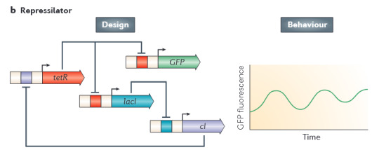
Repressilator. A circuit in which lacI represses cI, cI represses tetR, and tetR represses both lacI and GFP. In each cell, a signal of repression travels through the whole circuit: the repression of tetR allows the expression of lacI, which represses cI, which reactivates tetR, and vice versa. The expression of GFP, and therefore the cell fluorescence, fluctuates over time in a regular cycle.

Purpose: gene expression that cycles over time.

Autoregulatory circuit. The gene tetR, concatenated to GFP, represses its own expression. Whenever too much tetR and GFP are produced, the expression regulates itself down, so that in a large population there is much less variation in fluorescence: all cells converge to a moderate value. (remember?)

Purpose: gene expression that is kept moderated in a population of cells.

Modular riboregulator. Control acting later in gene expression: not on DNA -> RNA transcription, but on RNA -> protein translation. Transcribed GFP is connected to a sequence that inhibits translation by folding over and preventing the ribosome from attaching to the RNA. A separated activator RNA binds to this sequence and prevents it from preventing translation.

Purpose: a second tier of control over gene expression.

Two-input AND gate. Logic gates with genes! Expression of GFP requires a promoter encoded in T7, which in turn is only expressed in the presence of arabinose. However, the promoter only works if it's modified by by RNA produced by supO, which is only expressed in the presence of salicylate. Therefore, GFP is only produced if both arabinose and salicylate are present at the same time.

Purpose: protein synthesis that only occurs if multiple conditions are verified.

Multicellular pattern formation. This one is meant to be used in large cell populations. The gene luxI in the "sender cell" encodes an enzyme that produces AHL, a signal molecule. This molecule may bind to LuxR receptors in the "receiver cells". LuxR binding AHL activates the expression of cI, which stops the expression of lacI, which stops the expression of GFP. However, lacI can also be directly activated by binding AHL, so that only an intermediate concentration of AHL results in producing the fluorescent protein. By adjusting the sensitivity of LuxR, GFP and RFP can be produced selectively at different concentrations of AHL, and therefore at different distances from the sender cell.

Purpose: spatial control of gene expression.

Relaxation oscillator. Similar in concept and purpose to the repressilator, but the cycle it creates is more stable and regular. araC activates GFP, lacI, and itself; lacI represses GFP, araC, and itself.

Recombinase-based logic. GFP is flanked by sequences that can be inverted by the recombinase enzymes Rec1 and Rec2 (Rec1 inverts whatever is between the blue boxes, and Rec2 what's between the orange boxes, respectively). Arranging the markers around GFP in different ways allows the construction of different logic gates. In the case of the AND gate, the transcription in the blue region is going in the wrong direction, and GFP is also backward; both recombinases must be active for GFP to be expressed. In the case of the OR gate, transcription begins in both the blue and the orange region, but goes in the wrong direction in both; it's sufficient for either to be inverted by one recombinase to express GFP. In the case of the NOR gate, transcription already proceeds well, as long as both recombinases are absent.

Purpose: construction of arbitrarly logical circuits; very precise conditional control of gene expression.

Edge-detection circuit. A modification of the quorum-sensing system used for the multicellular pattern. The cell colony is exposed to light, half-covered by an opaque mask. Cells in the dark express the luxI gene, producing the AHL signal, as well as cI; the sensor that activates the expression of these two genes turns off in the light. The gene lacZ leads to the production of a black pigment; it is activated by LuxR (the receptor of AHL), and repressed by cI. Therefore, the black pigment is only produced in cells exposed to light (no expression of cI) which are adjacent cells in the dark (low-sensitivity LuxR receiving AHL from neighbors).

Purpose: mark edges between areas with different conditions.

[violetfractal]

Violet is playing Microsoft Excel...

You're listening to an ms excel fractal played one column at a time! Imagine the spreadsheet is sheet music with higher pitches toward the bottom. (The pitch for each row is in column C.)

I made this sound in miscrosoft excel! I made it in desmos. I used excel to generate excel formulas that generate desmos formulas that play music.

I was inspired by this arcade machine i saw.

wanna see some formula gore?

https://www.desmos.com/calculator/ecyjwrrg63

the desmos code is generated by excel:

A261="\operatorname{tone}("&C2&",L_{"&(ROW()-259)&"}[\operatorname{mod}(o,l_{"&(ROW()-259)&"})])"

B261="l_{"&(ROW()-259)&"}=\operatorname{length}(L_{"&(ROW()-259)&"})"

C261="L_{"&(ROW()-259)&"}=["&D261&"0]"

D261=CONCATENATE ???

you can't ask excel 2010 for concatenate(a1:a3). it will only take concatenate(a1,a2,a3). So I had to generate a list of cells to concatenate.

??? was generated recursively by:

E260=ADDRESS(ROW()+1,COLUMN(),4,1) F260=E260&","&ADDRESS(ROW()+1,COLUMN(),4,1)

[communist-manifesto-daily]

Socialism: Utopian and Scientific - Part 24

[ First | Prev | Table of Contents | Next ]

To the metaphysician, things and their mental reflexes, ideas, are isolated, are to be considered one after the other and apart from each other, are objects of investigation fixed, rigid, given once for all. He thinks in absolutely irreconcilable antitheses. His communication is 'yea, yea; nay, nay'; for whatsoever is more than these cometh of evil." For him, a thing either exists or does not exist; a thing cannot at the same time be itself and something else. Positive and negative absolutely exclude one another; cause and effect stand in a rigid antithesis, one to the other.

At first sight, this mode of thinking seems to us very luminous, because it is that of so-called sound commonsense. Only sound commonsense, respectable fellow that he is, in the homely realm of his own four walls, has very wonderful adventures directly he ventures out into the wide world of research. And the metaphysical mode of thought, justifiable and necessary as it is in a number of domains whose extent varies according to the nature of the particular object of investigation, sooner or later reaches a limit, beyond which it becomes one-sided, restricted, abstract, lost in insoluble contradictions. In the contemplation of individual things, it forgets the connection between them; in the contemplation of their existence, it forgets the beginning and end of that existence; of their repose, it forgets their motion. It cannot see the woods for the trees.

For everyday purposes, we know and can say, e.g., whether an animal is alive or not. But, upon closer inquiry, we find that his is, in many cases, a very complex question, as the jurists know very well. They have cudgelled their brains in vain to discover a rational limit beyond which the killing of the child in its mother's womb is murder. It is just as impossible to determine absolutely the moment of death, for physiology proves that death is not an instantaneous, momentary phenomenon, but a very protracted process.

In like manner, every organized being is every moment the same and not the same; every moment, it assimilates matter supplied from without, and gets rid of other matter; every moment, some cells of its body die and others build themselves anew; in a longer or shorter time, the matter of its body is completely renewed, and is replaced by other molecules of matter, so that every organized being is always itself, and yet something other than itself.

Further, we find upon closer investigation that the two poles of an antithesis, positive and negative, e.g., are as inseparable as they are opposed, and that despite all their opposition, they mutually interpenetrate. And we find, in like manner, that cause and effect are conceptions which only hold good in their application to individual cases; but as soon as we consider the individual cases in their general connection with the universe as a whole, they run into each other, and they become confounded when we contemplate that universal action and reaction in which causes and effects are eternally changing places, so that what is effect here and now will be cause there and then, and vice versa.

None of these processes and modes of thought enters into the framework of metaphysical reasoning. Dialectics, on the other hand, comprehends things and their representations, ideas, in their essential connection, concatenation, motion, origin and ending. Such processes as those mentioned above are, therefore, so many corroborations of its own method of procedure.

Nature is the proof of dialectics, and it must be said for modern science that it has furnished this proof with very rich materials increasingly daily, and thus has shown that, in the last resort, Nature works dialectically and not metaphysically; that she does not move in the eternal oneness of a perpetually recurring circle, but goes through a real historical evolution. In this connection, Darwin must be named before all others. He dealt the metaphysical conception of Nature the heaviest blow by his proof that all organic beings, plants, animals, and man himself, are the products of a process of evolution going on through millions of years. But, the naturalists, who have learned to think dialectically, are few and far between, and this conflict of the results of discovery with preconceived modes of thinking, explains the endless confusion now reigning in theoretical natural science, the despair of teachers as well as learners, of authors and readers alike.

[ First | Prev | Table of Contents | Next ]

[pancakeke]

I genuinely could not figure out a normal way to make gsheets let me conditional format bingo card tiles that needed to be marked off so those sheets have a hidden tab that grabs all the tile options and uses TRIM to remove any potential trailing spaces from them. the tile options marked as hit have a single space added to the end via CONCATENATE. those modified tile options are then added to the card tab using WRAPCOLS, and finally conditional formatting highlights cells that end with spaces using =IF(RIGHT(A1,1)=" ",TRUE,FALSE)

[chiseld]

C is kicking my ass tonight :'( I seem to have forgotten some pretty basic stuff I thought I knew years ago. First, I couldn't get my code to correctly run the "strlen" function for so long that I got impatient and just wrote a string length function myself (I mean, it's easy enough, why not do it manually).

And then I got completely stuck while trying to concatenate characters one by one to an empty string after uppercasing each character. I presume the problem is that the non-existent string currently has garbage values in it, but I don't know how to handle that situation. Or could I somehow be using the "toupper" function wrong? Ugh, I don't know :/

Anyway, it completely fucked up my program – was clearly accessing memory it shouldn't be accessing, made my computer do a weird "bing" noise, etc. Not a great result :|

I see plenty of StackOverflow questions on this exact topic, but I don't want to use any techniques that we haven't already learned in this class so far, because I know we SHOULD be able to do it – it shouldn't be that hard. Blahhhh it's past midnight so I'll probably just call it night and come back with fresh eyes and brain cells tomorrow.

[scatter-brain-at-work]

id rather concatenate with you in a new cell

if we were cells in a spreadsheet would you merge with me

[aventurineswife]

PART A: PLANETS (THE CONCATENATION)

(from , meow anon. very fair warning: VERY LONG, NO BETA WE DIE LIKE THE CHRYSOS HEIRS /NSRS)

so we start off with the planets themselves, and YES, you read that right- planets plural. so we have leviathans in the canon lore, right. and generally, living beings can ascend to aeonhood, and we know that there was this ONE leviathan that did end up doing that. that was oroboros, the aeon of voracity.

its said that leviathans were wiped out after this huge war, but "during their lengthy slumber, their decomposed cells became the seedbed for organic organism, and their dissipating life force became wandering astral spirits. however, more and more scholars have begun to publicly denounce the leviathan's conception theory in recent years." there's a few more things that my friend sent abt leviathans here, but to put it simply, the planets ill talk about were created from the shed skin of the the aforementioned aeon

one big skin turned into nine fucking planets; the musvitan concatenation of planets, all based off the nine muses of greek mythology

the shed skin. is a core inside every single planet, sorta splitting apart into a non-solid form after the main body was like- it had a bunch of space debris be attracted to it, and it then formed a bigass fucking planet. that was kalioath, the very first of the nine

the rest came after some complications, because kalioath ended up being like 50% landmass and 50% core. it ended up oozing out the fucking ground and into space, which resulted into MORE space debris... and then more planets. aka the other eight nuisances /J

what does the core do? it directly creates these humanoid things called musvitans. musvitan singular

from the oldest to 'youngest' planet, it's in order like this:

kalioath (calliope; epic poetry)

klyo (clio; history)

polhymnus (polyhymnia; hymn, dance, and agriculture)

eythere (euterpe; general music and lyric poetry)

tersichor (terpsichore; dance and chorus)

kythar (erato; erotic poetry and mimic imitation)

melphimus (melpomene; tragedy)

talias (thalia; idyllic poetry)

uranyos (urania; astronomy)

the way it works is. weird. so imagine the core as a tree. the roots are in the center of the planet, and the numerous fruits at the end of its branches are COFFINS. they are BOXES that are EMBEDDED INTO THE GROUND.

the coffins are like numerous wombs, for lack of better phrasing. they adapt to their own environments and whatever, and slowly but surely, a person is being formed inside each one. after literally... nine months, same as pregnancy, the boxes move closer to the surface of the dirt and. grave robbing ensues, im not fucking kidding

but at FIRST, when the first musvitans were born, they just. pushed the lids off the box and started learning how to walk on their own. then it's just caveman shit from then on. they literally go through human development from the ground up, on their own.

mind you, if we're using the game's current timeline as a reference of the present, due to being born from oroboros' shed leviathan skin- they are OLDER than some of the CURRENT AEONS that we already know of ingame!! from playable to non-playable!! older than akivili the trailblaze, nanook the destruction, xipe the harmony, yaoshi the abundance, lan the hunt, nous the erudition, ix the nihility, all of these aeons. maybe not fuli, that feels impossible, but we just don't know enough about THEM to really say, yk?

so musvitans have had... all this time to improve themselves on their own, the real definition of the most independent planet inhabitants ever. and because of this, and because people are used to their own environments and have everything they could possibly need, they unintentionally became a recluse species. not once have they traveled past the concatenation of planets, because they're so self-assured that they don't need anyone else besides themselves.

but! there is a crucial thing that i forgot to fucking mention GSDHYAGHAHAHAH

so there are nine planets. right. out of nine planets, only three of them are actually still kicking around! to quote my friend who'd helped me plenty with the lore in terms of aligning it with canon events in the game's own lore, "so, in one of penacony’s side quests you’re introduced to this old guy called elias salas who turns out to be a member of the genius society. tldr, he’s being held captive in the dreamscape because of a nuclear(?) weapon testing incident gone wrong. he wiped out a fuckton of planets AND their inhabitants along with them."

and after this tragedy manage to topple six of the planets in the musvitan concatenation. this further solidified their isolation from the rest of the cosmos forever

part b will detail everything about the actual species 😭😭 i dont want you to read another hundred something words just yet, i js scrolled through to check if i missed anything and it feels so JALDJAKSHSSI??? LIKE. OML. also if any oomfs spot me. shhhhhh. shhhh ....

thank you for your time GSGAHAHAHA OH DEAR

First of all: Sorry for the late response, I have been too unmotivated to respond or do anything but I finally forced myself and here we are!

Secon of all: holy shit. This is an entire cosmology, and the sheer scope of it? Beautifully feral. You weren’t kidding about it being long, but it flows so naturally that it doesn’t feel long. The scale. The drama. The weird half-horrifying, half-elegant biology. I’m chewing glass in the best way.

Using Oroboros’ shed skin to seed an entire nine-planet system? That’s such an insane visual. It’s not just “dead god creates life” — it’s gross and sacred and planetary, which is such a powerful combo. I love how Kalioath sort of bleeds out into existence, and then chaos follows with the rest of the planets being like, “oh cool, we’re born of divine ooze and suffering? Let’s go.” The whole “coffin wombs” thing is terrifyingly beautiful — like, deeply Lovecraftian but flipped inside-out, with this elegant sci-fi coat of paint. Grave robbing as a birth rite? Iconic. Mythic. So deeply wrong it's right.

Also the idea that the musvitans never left their system because they just didn’t need to? That’s such an eerie and kind of tragic detail. Like they’ve had eons to develop, become ancient and refined and unknowably weird... but also became spiritually sedentary. It's such a haunting contrast to the Trailblazer-centric Star Rail theme of movement and journey.

And the three surviving planets? Tied to an in-game event?? The Elias Salas connection is insanely smart. You’re grounding your eldritch-scale headcanon in canon lore so well, it makes it feel like you just peeled back a hidden part of the game rather than made it up. I was nodding the entire time like “Yes. This tracks. This is real now.”

[bpaeducators]

📊 MASTER THESE 5 ADVANCED FORMULAS 🔥

Become the Excel Pro your team relies on:

✅ Textjoin – =TEXTJOIN(" ", TRUE, A2:D2) – Combine names, words, or data cleanly.

✅ Concatenate – =CONCATENATE(P2, " ", Q2) – Merge cells the old-school way (still works great!).

✅ Round – =ROUND(A3, B3)` – Clean your numbers fast.

✅ Roundup – =ROUNDUP(H3, L3)` – Always round UP like a boss.

✅ Int – =INT(O3)` – Chop off decimals instantly.

🚀 Work faster. Analyze smarter. Impress everyone.

💾 Save this NOW — you’ll need it!

👥 Tag an Excel buddy

👇 Drop a 📈 if you LOVE learning new formulas

🔔 Follow @Excelwithaj #bpaeducators for Excel glow-ups!

#ExcelMastery #ExcelHacks #AdvancedExcel #ExcelTipsAndTricks #ProductivityBoost #LearnExcel #OfficeHacks #SpreadsheetSkills #ExcelFormulas #InstagramLearning #ReelTips #anjsenglishhub #ExcelPro #BPA #BPAeducators

[fromdevcom]

There are hundreds of built-in functions in Microsoft Excel. Furthermore, you can use these functions together in different combinations to create powerful formulas. The ability to create formulas in Excel that solve complex problems is largely what makes the application so legendary. With that in mind, we will now look at 10 Excel functions that you should add to your repertoire. IFERROR The IF function is probably one of the most widely used functions among Excel pros. It is a logical function; if something is true then do something, otherwise do something else. The ‘IF’ function allows you to build metadata - a set of data used to describe other data. Those same pros that use ‘IF’ also use the ‘IFERROR’ function to handle errors in their formulas. We can use ‘IFERROR’ to specify an alternative value where a calculation might result in an error. Let’s look at the ‘IFERROR’ function’s syntax:                       =IFERROR(value, value-if-error) There are two arguments in this formula: ‘value’ and ‘value-if-error’. The ‘value’ argument is the parameter the function tests for an error. This is most often another formula itself. Then the ‘value-if-error’ argument is the replacement value the user has selected for ‘IFERROR’ to return if the ‘value’ parameter does result in an effort. The ‘value-if-error’ can be an actual static value such as a string or a number, but it can also itself be another formula. In the example that follows, we have an average price calculation in the ‘Average Price’ column. It is a simple division calculation that is susceptible to a divide by zero error (#DIV/0!). In cell D6, this is precisely what has happened. However, by using the ‘IFERROR’ function, we can ensure that the value ‘0’ gets returned to the cell in the case of an error. Note the improvement to our result for row 6 in cell E6. COUNTIF Another popular ‘IF’ based function is ‘COUNTIF’. This function counts cells in a range where some specified condition is met. The syntax is simple. There are two arguments: ‘range’ and ‘criteria’. The ‘range’ argument is the range in which you are searching for the ‘criteria’. The ‘criteria’ argument is the specific condition that needs to be met for the count                                  =COUNTIF(range, criteria) In the following example, we use ‘COUNTIF’ to count the number of employees by their years of service. Our ‘range’ argument is the column containing the ‘Year of Service’ for each employee, or “D2: D19” (the dollar signs preceding the column and row references are simply there to ‘lock’ the range for dragging the formula to other cells). The ‘criteria’ argument is the years of service (1, 2 or 3). We could have placed the literal number values for ‘Years of Service’ as our ‘criteria’, but in this case, we opted to use the cell references for each (“F3”, “F4”, and “F5”, respectively). The ‘COUNTIF’ formula in each returns the count of employees corresponding to each value in ‘Years of Service’ in column G. Note the formulas for each row in column H. CONCATENATE The ‘CONCATENATE’ function is one of the most widely used in Excel. A point worth noting is that Microsoft introduced two new functions in Excel 2016 that will eventually replace ‘CONCATENATE’. They are ‘CONCAT’, a more flexible version of its predecessor, and ‘TEXTJOIN’. However, since not all Excel users have upgraded to Excel 2016, we will look at ‘CONCATENATE’. The ‘CONCATENATE’ function combines strings of text and/or numerical values. Syntactically, this simply means placing the values you want to concatenate in sequential order, separated by commas. You can use either literal values or cell references as your arguments. You can use a combination of both as well.                                         =CONCATENATE(text1,[text2],…) In the following example, we have two separate lists: first names and last names. Using the ‘CONCATENATE’ function, we will combine them in a column where we have the last name, then the first name separated by a comma.

Then we can sort each by the last name in alphabetical order. VLOOKUP If you have spent much time with anyone with a reasonable amount of proficiency using Excel, you have likely heard of ‘VLOOKUP’. Like its sibling, ‘HLOOKUP’, it will search a table of values based on a criteria value. The ‘VLOOKUP’ function will search the first column of a table for a criteria value and return a value from some specified number of columns to the right of that first column. The function consists of four arguments.                  =VLOOKUP(lookup_value, table_array, col_index_number, [range_lookup]) The first argument is the ‘lookup_value’ is the value ‘VLOOKUP’ seeks a match for in the ‘table_array’ argument. In the following example, this is the cell reference ‘E2’ where we see the string ‘Finance’. We could have just as easily used the literal string ‘Finance’ as our ‘lookup_value’ argument. But using the cell reference allows us to change the value in ‘E2’ without changing the formula. The ‘table_array’ is the table of values ‘VLOOKUP’ will seek a match for ‘Finance’ in the first column. Since our table is ‘A2: C7’, the match for our ‘lookup_value’ is on the first row (cell ‘A2’) of our ‘table_array’, The ‘col_index_number’ argument is the number of the column from which we want ‘VLOOKUP’ to return a match on the same row from the ‘lookup_value’. In our case, we want ‘Average Years of Service’ in our formula in cell ���F2’. This means we will insert ‘2’ as our ‘col_index_number’ argument since ‘Average Years of Service’ is the second column in our ‘table_array’. The ‘range_lookup’ argument is an optional argument as denoted by the square brackets. This argument can be one of two values: TRUE or FALSE. A TRUE value tells the ‘VLOOKUP’ to return an approximate match while a FALSE value tells it to return an exact match. When omitted, the default for the formula is an approximate match. In the following example, we can easily look up the average years of service and the average salary for employees by specifying the department. An insider trick regarding ‘range_lookup’: try using ‘1’ and ‘0’ as a substitute for TRUE and FALSE, respectively. This is a shortcut that works just the same. Note in ‘G2’ our ‘VLOOKUP’ uses ‘0’ instead of FALSE. INDEX And MATCH The combination of ‘INDEX’ and ‘MATCH’ function gives users the ability to retrieve data from a table by specifying the row and column condition. Combining the two in a single formula creates one of the most well-known lookup formulas used. The most basic example of what the ‘INDEX’ function does is that it takes an array, like a column of names. Then it takes a second argument, ‘row_num’, and returns the value from the array on that row.                                       =INDEX(array, row_num, [column_num]) Note that since we are working with a single column, we omit the optional ‘column_num’ argument since it is implied. However, if we were working with an array that had more than one column, we would use the ‘column_num’ argument in the same way we use the ‘row_num’ argument. ‘INDEX’ will return the value at the intersection of the two in the specified ‘array’. In the following example, the ‘column_num’ is understood to be 1. This means the formula finds the value at the intersection of row 6 and column 1 of our ‘array’, ‘A2: A19’. The ‘MATCH’ function takes a ‘lookup_value’, a ‘lookup_array’, and an optional ‘match_type’ argument. The ‘match_type’ argument allows for one of three values; ‘-1’ for less than, ‘0’ for an exact match, or ‘1’ for greater than.                      =MATCH(lookup_value, lookup_array, [match_type]) In the next example, we pass in a string value for the ‘lookup_value’ and ‘0’ to ‘match_type’ for an exact match. See cell ‘C12’ for the result. Now you have seen how you can find the row on which a value exists in a column using the ‘MATCH’ function. You have also seen how you can find the value in a cell by passing in a row number to the ‘INDEX’ function.

Imagine you had a second column with email addresses that you wanted to look up by employee name. See if you can figure out how to combine ‘INDEX’ with ‘MATCH’ to do just that. Hint: substitute the ‘MATCH’ formula for the ‘row_num’ argument in the ‘INDEX’ formula – then make sure you select the email column as the ‘array’ for your ‘INDEX’ function. GETPIVOTDATA If you have ever tried referring to a cell or range in a Pivot Table, you have probably seen ‘GETPIVOTDATA’. The GETPIVOTDATA function helps retrieve data from a pivot table using the corresponding row and column value. This function is yet another type of lookup function but for Pivot Table users. It provides a direct method of retrieving tabulated data from Pivot Tables.                  =GETPIVOTDATA(data_field ,pivot_table, [field1, item1], …) The first argument, ‘data_field’, refers to the data field from which we want our result. In the following example, this will be our Pivot Table columns. The second argument, ‘pivot_table’, refers to the actual Pivot Table. In the following example, this is simply the cell reference ‘I3’, which is cell where our Pivot Table originates. The third and fourth arguments, ‘field1’ and ‘item1’, refer to the field and row on which we want a match in the ‘data_field’. In our example below, our first ‘GETPIVOTDATA’ formula is looking for a match to the finance department in the ‘Average of Years of Service’ column. Note that instead of hard-coding the literal value ‘Finance’ for the ‘item1’ argument, we have used the cell reference ‘N4’ where we have entered that string value. Just as we have seen with the other formulas we have covered, literal values or cell references can be used. TEXTJOIN We alluded to one of the newest functions in Excel, ‘TEXTJOIN’, in our earlier discussion about ‘CONCATENATE’. This function is only available in Excel 2016 desktop or in Excel online as a part of Microsoft 365. Recall that the ‘CONCATENATE’ function requires an individual cell reference for each string. However, the ‘TEXTJOIN’ function allows you to combine strings by referring to multiple cells in a range. Usage of the ‘TEXTJOIN’ function is simple. There are three arguments.                                    =TEXTJOIN(delimiter, ignore_empty, text1, …) The first argument, ‘delimiter’, is any string you want to be placed between the joined elements. This could be a symbol like a comma(“,”), or it could be a space (“ “). If you want nothing between the string elements you are joining, you still must specify that with the ‘delimiter’ argument. You simply insert two double quotes with nothing in between (“”). The second argument, ‘ignore_empty’, allows you to tell the function whether you want to skip over empty cells when joining their values. This is simply a TRUE value for ignoring blanks, or FALSE when you do not want to ignore blanks. The ‘text1’ argument is simply the cell or range of values you want to join. One thing to note is that you can add multiple ‘text’ arguments for each cell or range you want to be a part of the ‘TEXTJOIN’ formula. Notice that we have a few blank cells in our range “A2: A19” but since we chose TRUE for the ‘ignore_empty’ argument, our result in the merged range “C2: G10” indicates no missing values between any of the commas. FORMULATEXT The ‘FORMULATEXT’ function returns the formula for a specific cell reference. If a formula is not present, the error value ‘#N/A’ results. This function provides an alternative way to visualize the formula present in a cell. The syntax is incredibly simple:                                           =FORMULATEXT(reference) The single argument, ‘reference’, is the cell reference where the formula exists. In the following example, there are multiplication formulas in column C. Placing a ‘FORMULATEXT’ function in the D column that references the cells on the same row in C, we can now visualize the formula as well as the result. IFS Another of the new functions available with Excel 2016 and Excel Online is the ‘IFS’ function.

This function works in similar fashion as the ‘IF’ function, but it goes further by providing an efficient method of incorporating multiple logical tests and multiple values. Where in the past the same results would require nested ‘IF’ functions, the ‘IFS’ simplifies this process.                                              =IFS(logical_test1, value_if_true1, ...) In this example, we can assign a description of performance without utilizing nested IF statements. Download Sample File  With the hundreds of available built-in functions with which to build your own formulas with, this list is by no means comprehensive. Furthermore, some of the functions on this list may not even resonate with your needs. However, we curated the list with broad appeal in mind and feel that most Excel users could find a way to leverage these at some point. Sometimes the simplest functions lead to formulas that create great value. Moreover, sometimes it is difficult to know what is possible until you see them in action. We hope you find this list helpful and inspiring! 

[mastersidlethoughts2]

Baby, I want to concatenate our cells

[harmonyos-next]

How to use HarmonyOS NEXT - Grid Layout?

Grid layout is composed of cells separated by rows and columns, and various layouts are made by specifying the cells where the items are located. Grid layout has strong ability to evenly distribute pages and control the proportion of sub components, making it an important adaptive layout. Its usage scenarios include nine grid image display, calendar, calculator, etc.

ArkUI provides Grid container components and sub components GridItem for building grid layouts. Grid is used to set parameters related to grid layout, and GridItem defines features related to sub components. The Grid component supports generating sub components using conditional rendering, loop rendering, lazy loading, and other methods.

interface [code] Grid(scroller?: Scroller, layoutOptions?: GridLayoutOptions) [/code]

The Grid component can be divided into three layout scenarios based on the number of rows and columns and the proportion attribute settings: ·Simultaneously set the number and proportion of rows and columns: Grid only displays elements with a fixed number of rows and columns, and does not display other elements. Additionally, Grid cannot be scrolled. (Recommended to use this layout method) ·Only set one of the number and proportion of rows and columns: elements are arranged according to the set direction, and any excess elements can be displayed by scrolling. ·The number and proportion of rows and columns are not set: elements are arranged in the layout direction, and the number of rows and columns is determined by multiple attributes such as the layout direction and the width of a single grid. Elements beyond the capacity of rows and columns are not displayed, and the Grid cannot be scrolled.

The overall arrangement of the grid layout can be determined by setting the number of rows and the proportion of sizes. The Grid component provides rowsTemplate and columnsTemplate properties for setting the number and size ratio of rows and columns in the grid layout. The rowsTemplate and columnsTemplate property values are a string composed of multiple spaces and 'numbers+fr' intervals concatenated together. The number of fr is the number of rows or columns in the grid layout, and the size of the value before fr is used to calculate the proportion of the row or column in the grid layout width, ultimately determining the width of the row or column.

The horizontal spacing between two grid cells is called row spacing, and the vertical spacing between grids is called column spacing The row column spacing of the grid layout can be set through the rowsGap and columnsGap of Grid

Code Example: GridPage [code] @Entry @Component struct GridPage { @State message: string = 'GridPage';

@Styles gridItemStyle(){ .backgroundColor(Color.Orange) // .margin(4) }

build() { Column() { Text(this.message) .fontSize(30) .fontWeight(FontWeight.Bold) Grid(){ GridItem(){ Text('1') }.gridItemStyle() GridItem(){ Text('2') }.gridItemStyle() GridItem(){ Text('3') }.gridItemStyle() GridItem(){ Text('4') }.gridItemStyle() GridItem(){ Text('5') }.gridItemStyle() GridItem(){ Text('6') }.gridItemStyle() GridItem(){ Text('7') }.gridItemStyle() GridItem(){ Text('8') }.gridItemStyle() GridItem(){ Text('9') }.gridItemStyle() } .size({width:300,height:300}) .rowsTemplate('1fr 1fr 1fr') .columnsTemplate('1fr 2fr 1fr') .backgroundColor('#EEEEEE') .padding(10) .columnsGap(10) .rowsGap(10) } .height('100%') .width('100%')

} } [/code]

performance optimization ·Similar to processing long lists, loop rendering is suitable for layout scenes with small amounts of data. When building a scrollable grid layout with a large number of grid items, it is recommended to use data lazy loading to iteratively load data on demand, thereby improving list performance. ·When using lazy loading to render a grid, in order to provide a better scrolling experience and reduce the occurrence of white blocks during sliding, the Grid component can also set the preloading quantity of GridItems through the cached count property, which only takes effect in lazy loading LazyForEach. ·After setting the preload quantity, several GridItems will be cached in the cached Count * columns before and after the Grid display area. GridItems that exceed the display and caching range will be released.

Code Examples [code] Grid() { LazyForEach(this.dataSource, () => { GridItem() { } }) } .cachedCount(3) [/code]

[tccicomputercoaching]

What Are the 7 Basic Excel Formulas?

Excel is a versatile tool used for data analysis, accounting, and day-to-day calculations. Mastering its basic formulas is a must for students and professionals alike. At TCCI Computer Coaching Institute, we guide you in understanding these essential formulas to enhance your productivity and efficiency.

SUMs

Formula: =SUM(A1:A10)

The SUM formula sums a range of numbers. It is excellent for summing up totals in budgets, invoices, or any dataset.

AVERAGE

Formula: =AVERAGE(A1:A10)

This computes the mean of a range of values, which will help you find the average sales, marks, or performance metrics.

IF

Formula: =IF(A1>50, "Pass", "Fail")

The IF function tests a condition and returns a value depending on whether the condition is TRUE or FALSE. It is very commonly used for decision-making scenarios in Excel.

VLOOKUP

Formula: =VLOOKUP(lookup_value, table_array, col_index, [range_lookup])

This formula is helpful in extracting data from a specified column in a table. This is useful for finding the price of a product or employee information.

HLOOKUP

Formula: =HLOOKUP(lookup_value, table_array, row_index, [range_lookup])

It is very similar to VLOOKUP, but it looks horizontally instead of vertically. It's useful for pulling information from a row instead of a column.

CONCATENATE / CONCAT

Formula: =CONCATENATE(A1, " ", B1) or =CONCAT(A1, " ", B1)

This combines data from multiple cells into one, which is great for creating full names or combining addresses.

NOW

Formula: =NOW()

This will display the current date and time. It's particularly useful for tracking timestamps or creating dynamic date-based reports.

Why Learn Excel at TCCI?

At TCCI Computer Coaching Institute, we offer extensive, hands-on training where you can master Excel formula and tools. We adapt our courses to suit everyone, whether you are a student, accountant, or data analyst.

Start with your Excel journey today by joining TCCI and getting your computer skills to even greater heights!

Call now on +91 9825618292

Get information from https://tccicomputercoaching.wordpress.com/

[esscomputerinstitute]

Top 10 Excel Tricks You Should Know

Excel is a versatile tool widely used for data management, analysis, and visualisation. As part of the Microsoft Office suite, Excel is indispensable for students and professionals, offering a platform to organise and process information efficiently. Its ability to perform calculations, create charts, and handle large datasets makes it an essential skill in academics, business, and everyday problem-solving. If you want to enhance your skills, learning these 10 tricks will make your work easier and more efficient.

1. Use Pivot Tables to Summarise Data

Pivot Tables help you quickly summarise large datasets. Instead of manually calculating totals or averages, you can use this tool to analyse your data with a few clicks. For example, if you have sales data for different regions, a Pivot Table can display total sales by region in seconds. Mastering Pivot Tables can give you an edge in any Excel course, as this feature is highly valued in data analysis.

2. Split Data into Separate Columns

When you have combined data, like full names or addresses, in one column, you can split it into multiple columns using the “Text to Columns” feature. Go to the “Data” tab, click “Text to Columns,” and choose how you want to split the data, such as by space or comma. This trick is especially useful for cleaning datasets before working on projects or assignments.

3. Transpose Rows and Columns

Need to switch rows into columns or vice versa? The transpose feature saves time and effort. Copy your data, right-click where you want to paste it and select “Transpose.” This simple trick is handy for reorganising data layouts.

4. Apply Conditional Formatting

Conditional Formatting highlights cells based on specific criteria. For instance, you can make all cells with marks above 90 turn green. Select your data, go to “Home” > “Conditional Formatting,” and set your rules. This trick helps you visually track trends or patterns in your data.

5. Remove Duplicate Data

Removing duplicates makes sure that your data is accurate and free from redundancy. Highlight the relevant column, go to the “Data” tab, and click “Remove Duplicates.” This trick is essential for students dealing with multiple datasets, such as when merging survey results or reports.

6. Use the IF Formula for Logical Conditions

The IF formula allows you to create logical conditions. For example, you can use it to check if marks are above a certain threshold and assign a grade accordingly. The formula format is =IF(condition, value_if_true, value_if_false). Learning this formula in an advance Excel course will help you automate repetitive tasks.

7. Leverage VLOOKUP to Find Data

VLOOKUP (Vertical Lookup) is useful when you need to search for data in a table. For example, if you have a list of student IDs and want to match them with their names, VLOOKUP can retrieve the relevant information instantly. It is an invaluable tool for assignments that involve cross-referencing data.

8. Use Filters to Simplify Data

Filters allow you to display only the rows you need. Click on the “Data” tab, select “Filter,” and use the dropdown options in each column to sort or filter your data. Filters are perfect for students working with large datasets, enabling them to focus on specific categories, such as filtering out overdue tasks.

9. Combine Text with the CONCATENATE Function

The CONCATENATE function merges text from multiple cells into one. For instance, if you have separate columns for first and last names, you can combine them into a full name using =CONCATENATE(A1, “ “, B1). This trick is particularly useful for creating clean, professional datasets.

10. Lock Cells with Absolute References

You might want specific cell references to remain constant when working with formulas, even when the formula is copied. Adding a dollar sign ($) before the column and row (e.g., $A$1) locks the reference. This trick prevents calculation errors, making it a fundamental concept covered in any Excel course.

Why Should You Learn These Tricks?

Mastering these Excel tricks will help you work smarter, not harder. These skills are invaluable for students in any field, from managing complex datasets to automating repetitive tasks. By enrolling in an advance Excel institute like ESS Institute, you can gain practical experience and build expertise in advanced features that will make your assignments and projects stand out. These tips are just the beginning. If you want to become proficient and gain an edge in academics or your career, it is time to invest in learning Excel.

Explore an advance Excel course at ESS Institute to unlock the full potential of this powerful tool!

[virtualemployeeblog]

Top 5 Excel Functions Every Expert Should Master 

Mastery of any data analysis tool like Excel comes with an addition to productivity and efficiency that is very significant. You can hire Microsoft excel experts who are experts in these functions: 

VLOOKUP- This function finds an item in a table or range and returns the corresponding value in another column. It is very helpful for the process of data lookup as well as matching. 

SUMIF - Sum cells in range that meet certain conditions. It is very commonly applied for filtering, aggregation, or calculation of data; for instance, it will sum up the sales within a specific type of product. 

COUNTIF - Like SUMIF, it counts the number of cells within a given range that meets criteria. It is helpful in running data analysis and also in reporting. 

IF - This function is designed to produce a logical test. Once this test becomes true, then it will yield some values; else it will yield different values. It plays a crucial role in formulating conditional formulas and making decisions. 

CONCATENATE - This function takes one or more text strings and returns them as a single text string. It's extremely useful when creating custom labels, reports, or indeed any other type of text-based output. Using CONCATENATE, you can take separate columns for first and last names and create one single name column with them. 

Anyone who is preparing for excel programmers for hire purposes must know these functions to tackle different types of data analysis jobs in the competitive landscape. 

[datawitzz]

How to combine text in Excel | TEXTJOIN function in Excel

How to combine text in excel Combining text in excel from different cells can be done in different ways. We can use ‘&’ to combine or can use CONCATENATE or CONCAT function to combine texts from different cells. But in all these methods when we are using some delimiters we need to put delimiter multiple times with every text also there was no provision of treating blank cells. How to combine…