#counta function

[techalertr]

Fantastic combination of Sequence and CountA functions to ease your work Full video on : https://youtu.be/l4SmyXEwgFg #techalert #excel #shorts #technical #howto #reels #instagram #howto #fbreels #trending #viral

[charl0ttan]

i have a sheet in this spreadsheet that lists all the albums ive rated for each genre and i want another sheet to have a list of the number of albums in each column using the counta function. but like i need to autofill it so that it takes the successive genre column for each row in the count spreadsheet. does anyone have any ideas. help lol🫶🦌

[000marie198]

He will overeat

And then get sick. It takes a while to get used to some fresh food which was otherwise synthesized and the kid often has to hold himself back. It doesn't help that his brothers like to spoil him and offer everything, how could he refuse *proceeds to get sick again*

Sometimes I forget that tasteless and/or synthetic food in New Yoke is nowhere confirmed canon, but just hear me out.

Nine is used to food just being a necessity that is not particularly enjoyable but important to have to be able to work properly, so when he sits down once in Green Hill and actually eats something with Seasoning and Spices and Texture and Flavor he obviously gets a bad case of tummy hurty(TM) (because his body is not used to processing Fresh Things) but before that he makes this exact face

[onecooooooolcat]

a filter function nestled in a counta function is like if the countifs function actually served cunt

[fromdevcom]

Looking for list of excel formulas? We have a create a cheat sheet for excel formulas to help beginners. The excel Spreadsheet has number of functions which can be used to help you greatly enhance your abilities when it comes to performing day to day maths operations. With excel, you no longer have to waste time doing things manually. If you are new to excel, know that you can use it to find totals for any given column or a row of numbers and perform many more functions. To achieve this, excel uses formulas in cells to perform the different calculations. When starting a formula you need to know that every formula usually starts with an equal sign which can then be followed by a number, math operators and the functions. In addition to this article you may also find this ebook about Microsoft Excel : 101 Secrets Of A Microsoft Excel Addict Snapshot of The Cheat Sheet Please click on the image to see in bigger size. Get Access To Printable Useful Excel Formula Cheat Sheet (PDF Format) For Just a Tweet The Fromdev Cheatsheet for excel formula is available totally free in exchange of a tweet. Download Cheatsheet As soon as you tweet we will redirect you to the download page and you will be able to downloaded the cheatsheet to your computer. Reference Operators These refer to a cell or a group of cells. Reference operators are divided into two types including: union and range. As for a range reference, it can be defined as the cells between and also includes the reference. It includes 2 cell addresses that have been separated by a colon. On the other hand, a union reference refers to 2 or more references. It is made up of 2 or more cell addresses that have been separated by a comma. Excel Formulas That You Need To Familiarize Yourself With SUM Just as the name suggests, you can expect the SUM function to help you add 2 or more numbers. For further assistance, you can also use the cell references together with the formula. For as long as there are numbers in the reference cells, you can have as many numbers as possible added together. Example of SUM formula in excel =SUM(A1:B5) =SUM(5, 5) =SUM(A1, B1) COUNTA This function allows you to count the numbers of non-empty cells in a given range. What the function does is that it allows you to count cells that already have numbers together with any other characters found in the cells. The function works with all data types. Example of COUNTA formula in excel =COUNTA(A1:A10) COUNT You can use the formula function to count the numbers of the different cells in a range that have numbers in them. The formula cannot work without numbers. Example of COUNT formula in excel =COUNT(A1:A10) TRIM This is a very useful function that was designed to help users get rid of any sorts of spaces found in cells. The only exception is with single spaces between words. Do not allow yourself to pull out data from your database with extra spaces because it can wreak havoc when it comes to comparing using IF statements or VLOOKUP's. Example Excel TRIM formula =TRIM(A1) LEN Whenever this function is included in a function, you can expect it to count the number of characters in that given cell. You need to note that this function also counts the spaces between words. If you do not need to count the spaces, do not use this function. Example Excel LEN formula =LEN(A1) VLOOKUP Anyone who has used excel for a while can attest to the fact that the VLOOKUP formula is the most used formula. What the formula really does is that it looks for a value that is found in the leftmost column of a table and goes ahead and returns a value in the same row from a column that you'd have specified. Below example searches for “TextToSearch” in array of cells from A1 to B10, the last parameter FALSE is used to do exact match search. Example Excel VLOOKUP formula =VLOOKUP("TextToSearch",A1:B10,2,FALSE) AVERAGE This function will help you to calculate the average value of the series of numbers found in between the specified cells.

In this case, the function will calculate the averages of the numbers found in the cells B1 to B3 and give you an optimal result. Example Excel AVERAGE formula =AVERAGE(B1:B3) MIN This function can be used to help one calculate the lowest number in a given series of numbers. In the example above, the formula will give you the lowest number found in the series between cells B1 to B3. Example MIN in excel formula =MIN(B1:B3) MAX The MAX function helps you to find the highest number in a given series of numbers. In the given example, the function will get you the highest figure in the series between cells B1 to B3. Example MAX in excel formula =MAX(B1:B3) IF Function You can use this function to help you determine whether a given statement is true or false which can then allow you to perform a specified action based on your results. Example IF in excel formula =IF(Criteria,True value,False value) SUMIF Function More or less similar to the IF Function. The only difference is that with the SUMIF Function, after finding the values of the set criteria, it will go ahead and Sum up the values of the related cells. Example SUMIF in excel formula Below example will do the sum of all number in A1 to A25 if they are greater than 10 =SUMIF(A1:A25,">10") COUNTIF Function The function works the same way as the SUMIF Function with the exception that it counts the fields that match with one another in relation to the set criteria instead of summing them together. Below example will do the count of all number in A1 to A25 if they are greater than 10 Example COUNTIF in excel formula =COUNTIF(A1:A255,">10") AND Function Dubbed as a logical function, the AND function helps you to check specified multiple criteria and will give a TRUE value if say ALL the criteria are found to be TRUE. If that criterion is not met, it will return as false. Below example will do logical AND operation of two conditions and return a boolean value. In this case it must return TRUE Example AND in excel formula =AND(1+1=2, 3+3=6) OR Function This function is similar to the AND Function. However, the OR Function checks multiple criteria but only requires ONE statement to be true for the entire statement to be TRUE. Below example will do logical OR operation of two conditions and return a boolean value. In this case it must return TRUE Example OR in excel formula =OR(1+1=2, 3+3=6) RIGHT, LEFT, MID Function All these functions are great TEXT functions that are used for manipulating data in a given cell. With the function, you can use it to take any numbers/words in a given cell, pull it in the right or left from them and go ahead to put them in a new cell. Example RIGHT in excel formula Example to get Right part of text, below will return TEXT =RIGHT('TESTSOMETEXT',4) Example LEFT in excel formula Example to get Left part of text, below will return TEST =LEFT('TESTSOMETEXT',4) Example MID in excel formula Example to get Middle part of text, below will return SOME =MID('TESTSOMETEXT',5,4 ) Jessica Millis, an aspiring writer and editor. Also Jess is working as an educator at JMU and as a chief editor at Essaymama essay writing agency. Article Updates Article Updated on September 2021. Some HTTP links are updated to HTTPS. Updated broken links with latest URLs. Some minor text updates done. Content validated and updated for relevance in 2021.

[dlbanalysis]

PowerBI Job Simulation - Histogram

So a while ago I completed the PwC Switzerland Job Simulation. I thought it was great actually, good to get really stuck in and start playing around with the data and making charts! In this post I wanted to talk about how I created a histogram to display the amount of calls answered within a certain duration, like this:

So, as none of the call centre staff have been selected this is displaying all calls by all people. But if we wanted to know specifically all calls answered by say, Greg, then we click on his name at the top:

We can clearly see that the histogram has changed and the Total Calls Answered amount at the bottom has now changed to reflect that of being filtered by Greg. So this is how I did it. Here is the DAX for the bins:

Bins = IF(CallCentreData[AvgTalkDuration] <= TIME(0,1,0), "00:01:00",

    IF(AND(CallCentreData[AvgTalkDuration] > TIME(0,1,0), CallCentreData[AvgTalkDuration] <= TIME(0,2,0)), "00:02:00",

    IF(AND(CallCentreData[AvgTalkDuration] > TIME(0,2,0), CallCentreData[AvgTalkDuration] <= TIME(0,3,0)), "00:03:00",

    IF(AND(CallCentreData[AvgTalkDuration] > TIME(0,3,0), CallCentreData[AvgTalkDuration] <= TIME(0,4,0)), "00:04:00",

    IF(AND(CallCentreData[AvgTalkDuration] > TIME(0,4,0), CallCentreData[AvgTalkDuration] <= TIME(0,5,0)), "00:05:00",

    IF(AND(CallCentreData[AvgTalkDuration] > TIME(0,5,0), CallCentreData[AvgTalkDuration] <= TIME(0,6,0)), "00:06:00",

    IF(AND(CallCentreData[AvgTalkDuration] > TIME(0,6,0), CallCentreData[AvgTalkDuration] <= TIME(0,7,0)), "00:07:00",

    IF(AND(CallCentreData[AvgTalkDuration] > TIME(0,7,0), CallCentreData[AvgTalkDuration] <= TIME(0,8,0)), "00:08:00")

    ))))))) The DAX TIME function takes three arguments and the syntax is TIME(hour, minute, second)

So basically what this is saying (using the first IF statement as an example), is that IF the average call duration is less than or equal to 1 minute, then put that entry into “00:01:00” in the Bins column. Everything else is where this test fails. The next conditions are strictly greater than the condition before it (i.e strictly greater than 1 minute but less than or equal to 2 and so on). This gives us the Histogram! So all these values would be plotted along the x-axis in 1 minute increments. The y-axis is calculated by this DAX measure: CallsAnswered = CALCULATE(COUNTA(CallCentreData[Answered (Y/N)]),CallCentreData[Answered (Y/N)] = "Y")

It was important to specify that the call had been answered because in the average call duration column – if the call wasn’t answered (i.e “N”) this would have no value in the average call duration – but because of how the above column had been calculated it would put in “00:01:00” ! (because it is technically less than or equal to 1?).

[korshubudemycoursesblog]

Mastering Microsoft Excel: From Basics to Advanced Techniques

Microsoft Excel has long been a staple in both personal and professional settings. Known for its powerful data manipulation capabilities, Excel is a versatile tool, suitable for everything from budgeting to complex data analysis. This guide is designed to take you on a journey through Microsoft Excel's core features, advanced techniques, and tips that will enhance your productivity, whether you're a beginner or a seasoned pro.

Why Learn Microsoft Excel?

Whether you're in finance, data science, marketing, or project management, Microsoft Excel skills are essential. In fact, employers often list Excel proficiency as a requirement, making it a valuable asset in the job market. Additionally, learning Microsoft Excel formulas and Excel functions can help streamline tasks, automate calculations, and make complex data more understandable.

Key Benefits of Mastering Microsoft Excel

Data Analysis: With Excel data analysis, you can easily organize, visualize, and interpret data.

Automation: Save time by learning Excel macros and automated workflows.

Visualization: The ability to create Excel charts and graphs provides insights at a glance.

Versatility: Excel templates and functions support a variety of tasks, from budgeting to project management.

Getting Started with Microsoft Excel Basics

If you’re new to Microsoft Excel, the interface might seem overwhelming, but a good starting point is understanding its core components.

The Ribbon: This is the toolbar across the top of the screen, housing essential tools and features.

Workbooks and Worksheets: An Excel workbook contains multiple worksheets, which are the individual pages where you enter data.

Cells and Cell References: Each worksheet has rows and columns that form cells, the building blocks for Excel data entry.

Fundamental Excel Formulas and Functions

Mastering Excel formulas is essential, as formulas are the backbone of calculations and data analysis in Excel. Here are some fundamental functions you need to know:

SUM Function: Used to add up values in cells, e.g., =SUM(A1:A5).

AVERAGE Function: Calculates the mean of a set of values, e.g., =AVERAGE(B1:B10).

IF Function: Enables conditional operations, e.g., =IF(A1>10, "Pass", "Fail").

VLOOKUP Function: Searches for a value in a table, e.g., =VLOOKUP("John", A2:B15, 2, FALSE).

COUNT and COUNTA Functions: Used to count cells with numbers (COUNT) or any content (COUNTA).

Tip: Practicing these basic functions will make learning Excel shortcuts and advanced formulas easier as you progress.

Excel Formatting Techniques for Better Presentation

In addition to calculations, Excel offers several formatting options to make data more readable:

Cell Formatting: Modify fonts, colors, and borders to organize and emphasize data.

Conditional Formatting: Use it to highlight cells based on criteria, making trends or outliers more visible.

Number Formatting: Format numbers as currency, percentage, date, etc., to improve data clarity.

Mastering these Excel formatting techniques helps you present information in a clear and effective way.

Advanced Features in Microsoft Excel

Once you have a firm grasp of the basics, diving into more advanced Excel features will significantly increase your efficiency and capabilities.

1. Pivot Tables: Simplify Large Data Sets

Pivot tables are powerful tools that allow you to summarize large datasets quickly. They make it easy to reorganize data without altering the original dataset, perfect for Excel data analysis.

To create a pivot table, select your data and choose "Insert" > "PivotTable." Drag fields into rows, columns, and values to customize your table.

Use filters to narrow down your view, helping you focus on relevant data points.

Learning to master Excel pivot tables can give you a solid edge in data handling.

2. Excel Macros: Automate Repetitive Tasks

For users who often perform repetitive tasks, learning Excel macros can save considerable time. Macros in Excel allow you to record sequences of actions and run them as a single command, automating your workflow.

To enable macros, go to the "Developer" tab, select "Record Macro," and perform the task you want to automate.

Macros are created in VBA (Visual Basic for Applications), Excel's programming language, allowing further customization for advanced users.

Using macros in Excel is an excellent way to boost productivity by reducing manual work.

3. Excel Charts and Data Visualization

Excel's charting tools make it easy to visualize data, turning rows of numbers into readable graphs. To create a chart:

Select your data.

Go to "Insert" > "Chart" and choose from a variety of options, like bar charts, line charts, and pie charts.

Customize your chart with labels, titles, and colors to make it more informative.

Common types of Excel charts include:

Pie Chart: Ideal for showing proportions.

Bar and Column Charts: Useful for comparing categories.

Line Chart: Great for trends over time.

Utilizing Excel data visualization can transform complex information into simple insights.

Mastering Excel Functions for Data Analysis

Once you’re familiar with basic functions, advanced Excel functions allow for deeper analysis.

1. INDEX and MATCH Functions: Alternative to VLOOKUP

INDEX and MATCH can replace VLOOKUP and offer more flexibility:

INDEX returns the value of a cell in a specified row and column.

MATCH provides the position of a value within a range.

Used together, =INDEX(B1:B10, MATCH("Value", A1:A10, 0)) allows more versatile lookups, even when data isn’t in the first column.

2. ARRAY Formulas: Efficient Data Calculations

Array formulas are advanced formulas that perform multiple calculations on one or more items in an array. Excel's recent updates now support dynamic arrays, allowing you to spill results across cells automatically. For example, {=SUM(A1:A10*B1:B10)} calculates a sum across both arrays.

Mastering Excel array formulas can significantly speed up your data analysis.

3. Power Query: Advanced Data Transformation

For those working with external data sources, Power Query in Excel is a game-changer. This feature lets you import, clean, and transform data from various sources, such as databases, web pages, and files, with ease.

Open Power Query via the "Data" tab.

Load data, clean it, and apply transformations (like removing duplicates).

Load the transformed data back into Excel for analysis.

Using Power Query can drastically simplify your data-cleaning tasks, making it a top skill for analysts.

Tips to Boost Productivity in Microsoft Excel

To work smarter and faster, mastering a few Excel shortcuts can make a big difference:

Ctrl + C/V/X: Copy, paste, cut.

Ctrl + Z/Y: Undo and redo.

Alt + =: Quickly adds a SUM formula.

F2: Edit the selected cell.

The Power of Excel Templates

To further streamline tasks, Excel templates provide pre-built layouts for common tasks like budgeting, project tracking, and calendars. Templates save setup time and offer consistent formatting across projects.

Practical Applications of Microsoft Excel in Various Fields

Excel for Finance and Accounting

Excel is a critical tool in finance for budgeting, forecasting, and data analysis. Excel finance functions, such as NPV (Net Present Value) and IRR (Internal Rate of Return), assist with investment analysis and financial modeling.

Excel for Data Analysis and Business Intelligence

In data science and BI, Microsoft Excel’s advanced formulas and features, like Power Pivot and data analysis toolpak, allow users to model and analyze datasets efficiently. Creating dashboards that aggregate data from multiple sources provides a clear view of key metrics.

Excel for Marketing Analytics

For marketing professionals, Excel is invaluable for customer segmentation, trend analysis, and report generation. Importing social media data, website analytics, and campaign performance metrics allows marketers to optimize strategies based on real-time insights.

Final Thoughts on Mastering Microsoft Excel

From beginners just getting started with Excel basics to advanced users leveraging macros and VBA for automation, Microsoft Excel remains one of the most powerful tools across industries. By exploring the features discussed in this guide, you’ll improve your productivity and gain new insights from data. Whether you’re creating PivotTables, mastering Excel data visualization, or automating processes with Excel macros, the possibilities with Microsoft Excel are vast.

[jvkings]

How to use the COUNTA function in Excel

[lifeinapic]

Looking for list of excel formulas? We have a create a cheat sheet for excel formulas to help beginners. The excel Spreadsheet has number of functions which can be used to help you greatly enhance your abilities when it comes to performing day to day maths operations. With excel, you no longer have to waste time doing things manually. If you are new to excel, know that you can use it to find totals for any given column or a row of numbers and perform many more functions. To achieve this, excel uses formulas in cells to perform the different calculations. When starting a formula you need to know that every formula usually starts with an equal sign which can then be followed by a number, math operators and the functions. In addition to this article you may also find this ebook about Microsoft Excel : 101 Secrets Of A Microsoft Excel Addict Snapshot of The Cheat Sheet Please click on the image to see in bigger size. Get Access To Printable Useful Excel Formula Cheat Sheet (PDF Format) For Just a Tweet The Fromdev Cheatsheet for excel formula is available totally free in exchange of a tweet. Download Cheatsheet As soon as you tweet we will redirect you to the download page and you will be able to downloaded the cheatsheet to your computer. Reference Operators These refer to a cell or a group of cells. Reference operators are divided into two types including: union and range. As for a range reference, it can be defined as the cells between and also includes the reference. It includes 2 cell addresses that have been separated by a colon. On the other hand, a union reference refers to 2 or more references. It is made up of 2 or more cell addresses that have been separated by a comma. Excel Formulas That You Need To Familiarize Yourself With SUM Just as the name suggests, you can expect the SUM function to help you add 2 or more numbers. For further assistance, you can also use the cell references together with the formula. For as long as there are numbers in the reference cells, you can have as many numbers as possible added together. Example of SUM formula in excel =SUM(A1:B5) =SUM(5, 5) =SUM(A1, B1) COUNTA This function allows you to count the numbers of non-empty cells in a given range. What the function does is that it allows you to count cells that already have numbers together with any other characters found in the cells. The function works with all data types. Example of COUNTA formula in excel =COUNTA(A1:A10) COUNT You can use the formula function to count the numbers of the different cells in a range that have numbers in them. The formula cannot work without numbers. Example of COUNT formula in excel =COUNT(A1:A10) TRIM This is a very useful function that was designed to help users get rid of any sorts of spaces found in cells. The only exception is with single spaces between words. Do not allow yourself to pull out data from your database with extra spaces because it can wreak havoc when it comes to comparing using IF statements or VLOOKUP's. Example Excel TRIM formula =TRIM(A1) LEN Whenever this function is included in a function, you can expect it to count the number of characters in that given cell. You need to note that this function also counts the spaces between words. If you do not need to count the spaces, do not use this function. Example Excel LEN formula =LEN(A1) VLOOKUP Anyone who has used excel for a while can attest to the fact that the VLOOKUP formula is the most used formula. What the formula really does is that it looks for a value that is found in the leftmost column of a table and goes ahead and returns a value in the same row from a column that you'd have specified. Below example searches for “TextToSearch” in array of cells from A1 to B10, the last parameter FALSE is used to do exact match search. Example Excel VLOOKUP formula =VLOOKUP("TextToSearch",A1:B10,2,FALSE) AVERAGE This function will help you to calculate the average value of the series of numbers found in between the specified cells.

In this case, the function will calculate the averages of the numbers found in the cells B1 to B3 and give you an optimal result. Example Excel AVERAGE formula =AVERAGE(B1:B3) MIN This function can be used to help one calculate the lowest number in a given series of numbers. In the example above, the formula will give you the lowest number found in the series between cells B1 to B3. Example MIN in excel formula =MIN(B1:B3) MAX The MAX function helps you to find the highest number in a given series of numbers. In the given example, the function will get you the highest figure in the series between cells B1 to B3. Example MAX in excel formula =MAX(B1:B3) IF Function You can use this function to help you determine whether a given statement is true or false which can then allow you to perform a specified action based on your results. Example IF in excel formula =IF(Criteria,True value,False value) SUMIF Function More or less similar to the IF Function. The only difference is that with the SUMIF Function, after finding the values of the set criteria, it will go ahead and Sum up the values of the related cells. Example SUMIF in excel formula Below example will do the sum of all number in A1 to A25 if they are greater than 10 =SUMIF(A1:A25,">10") COUNTIF Function The function works the same way as the SUMIF Function with the exception that it counts the fields that match with one another in relation to the set criteria instead of summing them together. Below example will do the count of all number in A1 to A25 if they are greater than 10 Example COUNTIF in excel formula =COUNTIF(A1:A255,">10") AND Function Dubbed as a logical function, the AND function helps you to check specified multiple criteria and will give a TRUE value if say ALL the criteria are found to be TRUE. If that criterion is not met, it will return as false. Below example will do logical AND operation of two conditions and return a boolean value. In this case it must return TRUE Example AND in excel formula =AND(1+1=2, 3+3=6) OR Function This function is similar to the AND Function. However, the OR Function checks multiple criteria but only requires ONE statement to be true for the entire statement to be TRUE. Below example will do logical OR operation of two conditions and return a boolean value. In this case it must return TRUE Example OR in excel formula =OR(1+1=2, 3+3=6) RIGHT, LEFT, MID Function All these functions are great TEXT functions that are used for manipulating data in a given cell. With the function, you can use it to take any numbers/words in a given cell, pull it in the right or left from them and go ahead to put them in a new cell. Example RIGHT in excel formula Example to get Right part of text, below will return TEXT =RIGHT('TESTSOMETEXT',4) Example LEFT in excel formula Example to get Left part of text, below will return TEST =LEFT('TESTSOMETEXT',4) Example MID in excel formula Example to get Middle part of text, below will return SOME =MID('TESTSOMETEXT',5,4 ) Jessica Millis, an aspiring writer and editor. Also Jess is working as an educator at JMU and as a chief editor at Essaymama essay writing agency. Article Updates Article Updated on September 2021. Some HTTP links are updated to HTTPS. Updated broken links with latest URLs. Some minor text updates done. Content validated and updated for relevance in 2021.

[krishnaacademyrewa]

Master 10 Basic Excel & Google Sheets Formulas in One Class! Enhance Your Spreadsheet skills!

Unlock the power of Excel and Google Sheets with Krishna Academy Rewa! In this class, we'll cover 10 essential formulas and functions that will help you master spreadsheet tasks with ease. Visit More : https://www.youtube.com/watch?v=TQb35cjMFzw

What You'll Learn:

1. SUM: Add up a range of numbers effortlessly.

2. COUNTA: Count the number of non-empty cells.

3. MAX & MIN: Find the highest and lowest values in your data.

4. AVERAGE: Calculate the mean value.

5. CONCATENATE: Combine text from multiple cells.

6. COUNT: Count the number of cells that contain numbers.

7. UPPER & LOWER: Convert text to uppercase or lowercase.

8. PROPER: Capitalize the first letter of each word. Why Join Us?

1. Expert Instruction: Learn from experienced professionals at Krishna Academy Rewa.

2. Hands-On Learning: Practical examples and exercises to help you understand and apply each function.

3. Versatile Skills: These formulas are crucial for various tasks in both Excel and Google Sheets.

Don't miss this opportunity to enhance your spreadsheet skills! Subscribe to our channel for more tutorials and visit Krishna Academy Rewa for advanced courses on computer applications. -

- - #excelformulas - #GoogleSheetsFormulas - #spreadsheettips - #exceltutorial - #googlesheetstutorial - #BasicExcelFunctions - #BasicGoogleSheetsFunctions - #KrishnaAcademyRewa - #excelforbeginners - #GoogleSheetsForBeginners - #learnexcel - #LearnGoogleSheets - #computereducation - #onlinelearning - #dataanalysis - #SpreadsheetTraining - #exceltips - #googlesheetstips

[skills-course]

Corporate Finance Institute – Advanced Excel Formulas and Functions LINK DOWNLOAD: https://skillscourse.net/corporate-finance-institute-advanced-excel-formulas-and-functions/?feed_id=1867&_unique_id=653f6b815f9c9 Corporate Finance Institute – Advanced Excel Formulas and Functions Description of Advanced Excel Formulas and Functions This advanced Excel course is designed to take Excel users to the next level by illustrating advanced functions and formulas. Understand how to reference data using INDEX and MATCH Manipulate text-string data using functions like RIGHT, CELL, LEN, and FIND Apply data analysis tools, like data tables and PivotTables Master charting features like creating a gauge chart Learn the most advanced formulas, functions, and types of financial analysis to be an Excel power user. This advanced Excel training course builds on our free Excel Fundamentals – Formulas for Finance. It is designed specifically for spreadsheet users who are already proficient and looking to take their skills to an advanced level. This advanced tutorial will help you become a world-class financial analyst for careers in investment banking, private equity, corporate development, equity research, and FP&A. By watching the instructor build all the formulas and functions right on your screen, you can easily pause, rewatch, and repeat exercises until you’ve mastered them. What You’ll Learn In Advanced Excel Formulas and Functions This advanced Excel training course starts with a blank spreadsheet and quickly dives into using combinations of functions and formulas to perform dynamic analysis. The main formulas & functions covered in this training course include: INDEX and MATCH IF with AND / OR OFFSET combined with other functions CHOOSE for creating scenarios INDIRECT combined with other functions XNPV and XIRR CELL, COUNTA, and MID functions combined together PMT, IPMT, and principal payment calculations The main types of data analysis in this advanced tutorial include: Data tables Pivot tables Column and line charts Stacked column charts Waterfall charts Gauge charts More courses from the same author: Corporate Finance Institute

[pcmcollege]

Sum IF, Count A, Count IF, Vlockup, Average IF

Sum IF, Count A, Count IF, Vlockup, Average IF, Roundup, Rounddown, Excel Formula in Bangla

Hello Everyone In this video we will learn : Sum IF, Count A, Count IF, Vlockup, Average IF, Roundup, Rounddown,  Excel Formula in Bangla,  In this video about : excel formula roundup, excel formula rounddown, sumif in excel, counta in excel, countif formula in excel,  Watch this video & learn about : vlockup formula in excel, average if excel, excel sumif, roundup excel formula, rounddown excel formula,  In This Tutorial about : sum if excel formula, counta excel formula, counta excel function, countif excel formula, vlockup excel formula,  In This Tutorial I Have Explained About : average if excel formula, excel formulas, excel formulas and functions, It’s Published By Technical Azad. Thanks For Watching and Don’t Forget to SUBSCRIBE!

[paschimchhatnai]

Sum IF, Count A, Count IF, Vlockup, Average IF, Roundup, Rounddown, Excel Formula in Bangla

Sum IF, Count A, Count IF, Vlockup, Average IF, Roundup, Rounddown, Excel Formula in Bangla

Hello Everyone In this video we will learn : Sum IF, Count A, Count IF, Vlockup, Average IF, Roundup, Rounddown,  Excel Formula in Bangla,  In this video about : excel formula roundup, excel formula rounddown, sumif in excel, counta in excel, countif formula in excel,  Watch this video & learn about : vlockup formula in excel, average if excel, excel sumif, roundup excel formula, rounddown excel formula,  In This Tutorial about : sum if excel formula, counta excel formula, counta excel function, countif excel formula, vlockup excel formula,  In This Tutorial I Have Explained About : average if excel formula, excel formulas, excel formulas and functions, It’s Published By Technical Azad. Thanks For Watching and Don’t Forget to SUBSCRIBE! https://www.youtube.com/watch?v=8N9KmnEwzTs&list=PLJRjbmlApcjGW52WIgXlALdqAHYGj8qa9&index=3

[fromdevcom]

Looking for list of excel formulas? We have a create a cheat sheet for excel formulas to help beginners. The excel Spreadsheet has number of functions which can be used to help you greatly enhance your abilities when it comes to performing day to day maths operations. With excel, you no longer have to waste time doing things manually. If you are new to excel, know that you can use it to find totals for any given column or a row of numbers and perform many more functions. To achieve this, excel uses formulas in cells to perform the different calculations. When starting a formula you need to know that every formula usually starts with an equal sign which can then be followed by a number, math operators and the functions. In addition to this article you may also find this ebook about Microsoft Excel : 101 Secrets Of A Microsoft Excel Addict Snapshot of The Cheat Sheet Please click on the image to see in bigger size. Get Access To Printable Useful Excel Formula Cheat Sheet (PDF Format) For Just a Tweet The Fromdev Cheatsheet for excel formula is available totally free in exchange of a tweet. Download Cheatsheet As soon as you tweet we will redirect you to the download page and you will be able to downloaded the cheatsheet to your computer. Reference Operators These refer to a cell or a group of cells. Reference operators are divided into two types including: union and range. As for a range reference, it can be defined as the cells between and also includes the reference. It includes 2 cell addresses that have been separated by a colon. On the other hand, a union reference refers to 2 or more references. It is made up of 2 or more cell addresses that have been separated by a comma. Excel Formulas That You Need To Familiarize Yourself With SUM Just as the name suggests, you can expect the SUM function to help you add 2 or more numbers. For further assistance, you can also use the cell references together with the formula. For as long as there are numbers in the reference cells, you can have as many numbers as possible added together. Example of SUM formula in excel =SUM(A1:B5) =SUM(5, 5) =SUM(A1, B1) COUNTA This function allows you to count the numbers of non-empty cells in a given range. What the function does is that it allows you to count cells that already have numbers together with any other characters found in the cells. The function works with all data types. Example of COUNTA formula in excel =COUNTA(A1:A10) COUNT You can use the formula function to count the numbers of the different cells in a range that have numbers in them. The formula cannot work without numbers. Example of COUNT formula in excel =COUNT(A1:A10) TRIM This is a very useful function that was designed to help users get rid of any sorts of spaces found in cells. The only exception is with single spaces between words. Do not allow yourself to pull out data from your database with extra spaces because it can wreak havoc when it comes to comparing using IF statements or VLOOKUP's. Example Excel TRIM formula =TRIM(A1) LEN Whenever this function is included in a function, you can expect it to count the number of characters in that given cell. You need to note that this function also counts the spaces between words. If you do not need to count the spaces, do not use this function. Example Excel LEN formula =LEN(A1) VLOOKUP Anyone who has used excel for a while can attest to the fact that the VLOOKUP formula is the most used formula. What the formula really does is that it looks for a value that is found in the leftmost column of a table and goes ahead and returns a value in the same row from a column that you'd have specified. Below example searches for “TextToSearch” in array of cells from A1 to B10, the last parameter FALSE is used to do exact match search. Example Excel VLOOKUP formula =VLOOKUP("TextToSearch",A1:B10,2,FALSE) AVERAGE This function will help you to calculate the average value of the series of numbers found in between the specified cells.

In this case, the function will calculate the averages of the numbers found in the cells B1 to B3 and give you an optimal result. Example Excel AVERAGE formula =AVERAGE(B1:B3) MIN This function can be used to help one calculate the lowest number in a given series of numbers. In the example above, the formula will give you the lowest number found in the series between cells B1 to B3. Example MIN in excel formula =MIN(B1:B3) MAX The MAX function helps you to find the highest number in a given series of numbers. In the given example, the function will get you the highest figure in the series between cells B1 to B3. Example MAX in excel formula =MAX(B1:B3) IF Function You can use this function to help you determine whether a given statement is true or false which can then allow you to perform a specified action based on your results. Example IF in excel formula =IF(Criteria,True value,False value) SUMIF Function More or less similar to the IF Function. The only difference is that with the SUMIF Function, after finding the values of the set criteria, it will go ahead and Sum up the values of the related cells. Example SUMIF in excel formula Below example will do the sum of all number in A1 to A25 if they are greater than 10 =SUMIF(A1:A25,">10") COUNTIF Function The function works the same way as the SUMIF Function with the exception that it counts the fields that match with one another in relation to the set criteria instead of summing them together. Below example will do the count of all number in A1 to A25 if they are greater than 10 Example COUNTIF in excel formula =COUNTIF(A1:A255,">10") AND Function Dubbed as a logical function, the AND function helps you to check specified multiple criteria and will give a TRUE value if say ALL the criteria are found to be TRUE. If that criterion is not met, it will return as false. Below example will do logical AND operation of two conditions and return a boolean value. In this case it must return TRUE Example AND in excel formula =AND(1+1=2, 3+3=6) OR Function This function is similar to the AND Function. However, the OR Function checks multiple criteria but only requires ONE statement to be true for the entire statement to be TRUE. Below example will do logical OR operation of two conditions and return a boolean value. In this case it must return TRUE Example OR in excel formula =OR(1+1=2, 3+3=6) RIGHT, LEFT, MID Function All these functions are great TEXT functions that are used for manipulating data in a given cell. With the function, you can use it to take any numbers/words in a given cell, pull it in the right or left from them and go ahead to put them in a new cell. Example RIGHT in excel formula Example to get Right part of text, below will return TEXT =RIGHT('TESTSOMETEXT',4) Example LEFT in excel formula Example to get Left part of text, below will return TEST =LEFT('TESTSOMETEXT',4) Example MID in excel formula Example to get Middle part of text, below will return SOME =MID('TESTSOMETEXT',5,4 ) Jessica Millis, an aspiring writer and editor. Also Jess is working as an educator at JMU and as a chief editor at Essaymama essay writing agency. Article Updates Article Updated on September 2021. Some HTTP links are updated to HTTPS. Updated broken links with latest URLs. Some minor text updates done. Content validated and updated for relevance in 2021.

[futuretechhub-in]

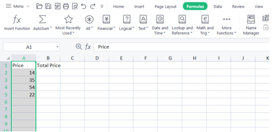
Dynamic Range : Dynamic Named Range in Excel

Unlock the power of Excel with dynamic named ranges and the OFFSET formula! Learn how to create dynamic ranges in Excel using the OFFSET function, allowing your spreadsheets to adapt automatically as data changes. Discover the flexibility and efficiency of dynamic named ranges, making your Excel sheets more versatile than ever. Master the art of dynamic named ranges in Excel today!

Dynamic Reach : Dynamic Named Reach in Succeed

List of chapters

Dynamic Named Reach in Succeed

This is an illustration of the way you can make a unique named range utilizing the OFFSET capability:

Dynamic Named Reach in Succeed

Adynamic named range is an element in bookkeeping sheet applications like Microsoft Succeed that permits you to make a named range whose size consequently changes in light of the information it contains. Dissimilar to a static named range, which has a proper scope of cells, a unique named range extends or contracts as information is added or eliminated.

Dynamic named range are especially helpful while working with huge datasets that are continually evolving. They can be utilized in different situations, for example, making outlines, utilizing recipes, or applying contingent arranging that consequently refreshes as new information is added.

To make a unique named range in Succeed, you can utilize a recipe joined with the OFFSET or List capability.

This is an illustration of the way you can make a unique named range utilizing the OFFSET capability:

Select the scope of cells that you need to powerfully name.

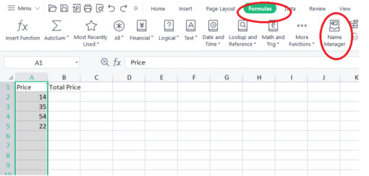
2. Go to the "Equations" tab in the Succeed lace and snap on "Characterize Name" (in more current adaptations of Succeed, this may be situated in the "Name Administrator" window).

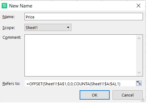
3. In the "New Name" discourse box, enter a name for your dynamic reach.

4. In the "Alludes to" field, enter the accompanying recipe utilizing the OFFSET capability:

=OFFSET(Sheet1!$A$1,0,0,COUNTA(Sheet1!$A:$A),1)

Supplant "Sheet1" with the name of your worksheet, and change the cell references on a case by case basis.

5. Click "Alright" to save the unique named range.

The recipe above utilizes the OFFSET capability to characterize a reach beginning from cell A1 and stretching out for various lines equivalent to the include of non-void cells in section A. The powerful named reach will refresh naturally as new information is added or eliminated in segment A.

You can utilize the made powerful named range in different Succeed highlights, for example, making diagrams or involving it in recipes like Total, Normal, or COUNT.

Succeed permits clients to characterize a powerful reach, which consequently changes in view of information changes, guaranteeing exact and adaptable information examination.

Note that the cycle might fluctuate somewhat relying upon the rendition of Succeed you are utilizing, however the idea continues as before — making a named range that changes progressively founded on the information.

See More Info :- https://futuretechhub.in/dynamic-range-dynamic-named-range-in-excel/

[futuretechhub]

Mastering Excel Efficiency: Unveiling Dynamic Named Range Hacks and Dynamic Ranges

Are you tired of constantly adjusting your data ranges in Excel spreadsheets, wondering if there's a better way to handle dynamic data? If you frequently work with large datasets that require constant updates, you may have found it challenging to maintain accurate references without constant manual intervention. But fear not! Excel offers an array of powerful hacks and tricks that can save you time, reduce errors, and enhance your productivity.

Understanding Dynamic Named Range Excel Formula

A Dynamic Named Range is a range name that automatically adjusts its size as the underlying data changes. This means that if you add or remove data from your spreadsheet, the named range will automatically expand or contract accordingly. This feature is exceptionally beneficial when creating formulas or charts that require consistent updates.

To create a dynamic named range, follow these steps:

Select the data range you want to name.

Click the "Formulas" tab in the Excel ribbon.

Choose "Define Name" in the "Defined Names" group.

In the "New Name" dialog box, provide a name for your range (avoid using spaces).

In the "Refers to" field, enter the following formula:

=OFFSET(Sheet1!$A$1,0,0,COUNTA(Sheet1!$A:$A),COUNTA(Sheet1!$1:$1))

Now, your named range is dynamic, and it will automatically adjust to include new data points in your spreadsheet. No more manual updates needed!

Excel's Dynamic Range Function

Apart from the dynamic named range, Excel also offers a built-in function called "INDEX" combined with "COUNTA" to create a "Dynamic Range Excel." With this method, you can create a formula that calculates the range based on the number of non-empty cells in a column.

The formula for a dynamic range using the INDEX and COUNTA functions is as follows:

=INDEX(Sheet1!$A:$A,1):INDEX(Sheet1!$A:$A,COUNTA(Sheet1!$A:$A))

Benefits of Using Dynamic Named Ranges and Dynamic Ranges

Simplified Formulas: By incorporating dynamic named range excel formula or dynamic ranges in your formulas, you won't have to worry about adjusting cell references when your data changes. This ensures greater accuracy and reduces the risk of errors.

Improved Data Validation: Dynamic named ranges are particularly useful when setting up data validation rules. Your drop-down lists will automatically include new entries without requiring manual updates.

Enhanced Charting and Reporting: With dynamic ranges, creating charts and generating reports becomes much more manageable. As your data grows, your visuals will automatically include the latest information.

Time Savings: The automatic adjustment feature of dynamic ranges eliminates the need for frequent manual interventions, saving you time and effort in the long run.

In conclusion, mastering the art of Dynamic Named Range and dynamic named range in excel can significantly boost your productivity and streamline your data management process. Embrace these Excel hacks, and you'll find yourself working more efficiently and accurately with your data, leaving you with more time to focus on what matters most. Happy Excel-ing!