#labelencoder

[damilola-doodles]

Project Title: Advanced recommender system with pandas.

# cddml-H7fJ3kLwQpR # File Name: advanced_recommender_system_with_pandas.py import numpy as np # type: ignore import pandas as pd # type: ignore import networkx as nx # type: ignore import matplotlib.pyplot as plt # type: ignore from sklearn.metrics.pairwise import cosine_similarity # type: ignore from sklearn.preprocessing import StandardScaler, LabelEncoder # type: ignore from sklearn.metrics…

[dammyanimation]

Project Title: Advanced recommender system with pandas.

# cddml-H7fJ3kLwQpR # File Name: advanced_recommender_system_with_pandas.py import numpy as np # type: ignore import pandas as pd # type: ignore import networkx as nx # type: ignore import matplotlib.pyplot as plt # type: ignore from sklearn.metrics.pairwise import cosine_similarity # type: ignore from sklearn.preprocessing import StandardScaler, LabelEncoder # type: ignore from sklearn.metrics…

[damilola-ai-automation]

Project Title: Advanced recommender system with pandas.

# cddml-H7fJ3kLwQpR # File Name: advanced_recommender_system_with_pandas.py import numpy as np # type: ignore import pandas as pd # type: ignore import networkx as nx # type: ignore import matplotlib.pyplot as plt # type: ignore from sklearn.metrics.pairwise import cosine_similarity # type: ignore from sklearn.preprocessing import StandardScaler, LabelEncoder # type: ignore from sklearn.metrics…

[damilola-warrior-mindset]

Project Title: Advanced recommender system with pandas.

# cddml-H7fJ3kLwQpR # File Name: advanced_recommender_system_with_pandas.py import numpy as np # type: ignore import pandas as pd # type: ignore import networkx as nx # type: ignore import matplotlib.pyplot as plt # type: ignore from sklearn.metrics.pairwise import cosine_similarity # type: ignore from sklearn.preprocessing import StandardScaler, LabelEncoder # type: ignore from sklearn.metrics…

[damilola-moyo]

Project Title: Advanced recommender system with pandas.

# cddml-H7fJ3kLwQpR # File Name: advanced_recommender_system_with_pandas.py import numpy as np # type: ignore import pandas as pd # type: ignore import networkx as nx # type: ignore import matplotlib.pyplot as plt # type: ignore from sklearn.metrics.pairwise import cosine_similarity # type: ignore from sklearn.preprocessing import StandardScaler, LabelEncoder # type: ignore from sklearn.metrics…

[learning-code-ficusoft]

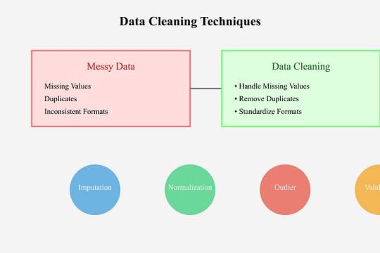
Data Cleaning Techniques Every Data Scientist Should Know

Data Cleaning Techniques Every Data Scientist Should Know 

Data cleaning is a vital step in any data analysis or machine learning workflow. Raw data is often messy, containing inaccuracies, missing values, and inconsistencies that can impact the quality of insights or the performance of models. 

Below, we outline essential data cleaning techniques that every data scientist should know. 

Handling Missing Values 

Missing data is a common issue in datasets and needs to be addressed carefully. 

Common approaches include: 

Removing Missing Data: 

If a row or column has too many missing values, it might be better to drop it entirely.

 python

 df.dropna(inplace=True) 

# Removes rows with any missing values Imputing Missing Data: 

Replace missing values with statistical measures like mean, median, or mode. 

python 

df[‘column’].fillna(df[‘column’].mean(), 

inplace=True)

 Using Predictive Imputation:

 Leverage machine learning models to predict and fill missing values. 

2. Removing Duplicates Duplicates can skew your analysis and result in biased models. 

Identify and remove them efficiently:

 python 

df.drop_duplicates(inplace=True) 

3. Handling Outliers 

Outliers can distort your analysis and lead to misleading conclusions. 

Techniques to handle them include:

 Visualization: Use boxplots or scatter plots to identify outliers. 

Clipping: Cap values that exceed a specific threshold. 

python

df[‘column’] = df[‘column’].clip(lower=lower_limit, upper=upper_limit) 

Transformation: Apply logarithmic or other transformations to normalize data. 

4. Standardizing and Normalizing 

Data To ensure consistency, particularly for machine learning algorithms, data should often be standardized or normalized: 

Standardization: Converts data to a mean of 0 and a standard deviation of 

python from sklearn.preprocessing 

import StandardScaler scaler = StandardScaler() 

df_scaled = scaler.fit_transform(df) 

Normalization: 

Scales values to a range between 0 and 1. 

pythonfrom sklearn.preprocessing 

import MinMaxScaler scaler = MinMaxScaler() 

df_normalized = scaler.fit_transform(df) 

5. Fixing Structural Errors

 Structural errors include inconsistent naming conventions, typos, or incorrect data types. 

Correct these issues by: Renaming columns for uniformity: 

python df.rename(columns={‘OldName’: ‘NewName’}, inplace=True) 

Correcting data types: 

python 

 df[‘column’] = df[‘column’].astype(‘int’) 

6. Encoding Categorical Data

 Many algorithms require numeric input, so categorical variables must be encoded: 

One-Hot Encoding: 

python

 pd.get_dummies(df, columns=[‘categorical_column’], drop_first=True) 

Label Encoding: 

python 

 from sklearn.preprocessing

 import LabelEncoder encoder = LabelEncoder()

 df[‘column’] = encoder.fit_transform(df[‘column’])

7. Addressing Multicollinearity

 Highly correlated features can confuse models.

 Use correlation matrices or Variance Inflation Factor (VIF) to identify and reduce multicollinearity. 

8. Scaling Large Datasets For datasets with varying scales, scaling ensures all features contribute equally to the model:

 python 

 from sklearn.preprocessing

 import StandardScaler scaler = StandardScaler()

 df_scaled = scaler.fit_transform(df) 

Tools for Data Cleaning 

Python Libraries: 

Pandas, NumPy, OpenRefine Automation: 

Libraries like dataprep or pyjanitor streamline the cleaning process. 

Visual Inspection: 

Tools like Tableau and Power BI help spot inconsistencies visually. Conclusion Data cleaning is the foundation of accurate data analysis and successful machine learning projects.

 Mastering these techniques ensures that your data is reliable, interpretable, and actionable.

 As a data scientist, developing an efficient data cleaning workflow is an investment in producing quality insights and impactful results.

[datasciencewithmohsin]

Feature Engineering in Machine Learning: A Beginner's Guide

Feature Engineering in Machine Learning: A Beginner's Guide

Feature engineering is one of the most critical aspects of machine learning and data science. It involves preparing raw data, transforming it into meaningful features, and optimizing it for use in machine learning models. Simply put, it’s all about making your data as informative and useful as possible.

In this article, we’re going to focus on feature transformation, a specific type of feature engineering. We’ll cover its types in detail, including:

1. Missing Value Imputation

2. Handling Categorical Data

3. Outlier Detection

4. Feature Scaling

Each topic will be explained in a simple and beginner-friendly way, followed by Python code examples so you can implement these techniques in your projects.

What is Feature Transformation?

Feature transformation is the process of modifying or optimizing features in a dataset. Why? Because raw data isn’t always machine-learning-friendly. For example:

Missing data can confuse your model.

Categorical data (like colors or cities) needs to be converted into numbers.

Outliers can skew your model’s predictions.

Different scales of features (e.g., age vs. income) can mess up distance-based algorithms like k-NN.

1. Missing Value Imputation

Missing values are common in datasets. They can happen due to various reasons: incomplete surveys, technical issues, or human errors. But machine learning models can’t handle missing data directly, so we need to fill or "impute" these gaps.

Techniques for Missing Value Imputation

1. Dropping Missing Values: This is the simplest method, but it’s risky. If you drop too many rows or columns, you might lose important information.

2. Mean, Median, or Mode Imputation: Replace missing values with the column’s mean (average), median (middle value), or mode (most frequent value).

3. Predictive Imputation: Use a model to predict the missing values based on other features.

Python Code Example:

import pandas as pd

from sklearn.impute import SimpleImputer

# Example dataset

data = {'Age': [25, 30, None, 22, 28], 'Salary': [50000, None, 55000, 52000, 58000]}

df = pd.DataFrame(data)

# Mean imputation

imputer = SimpleImputer(strategy='mean')

df['Age'] = imputer.fit_transform(df[['Age']])

df['Salary'] = imputer.fit_transform(df[['Salary']])

print("After Missing Value Imputation:\n", df)

Key Points:

Use mean/median imputation for numeric data.

Use mode imputation for categorical data.

Always check how much data is missing—if it’s too much, dropping rows might be better.

2. Handling Categorical Data

Categorical data is everywhere: gender, city names, product types. But machine learning algorithms require numerical inputs, so you’ll need to convert these categories into numbers.

Techniques for Handling Categorical Data

1. Label Encoding: Assign a unique number to each category. For example, Male = 0, Female = 1.

2. One-Hot Encoding: Create separate binary columns for each category. For instance, a “City” column with values [New York, Paris] becomes two columns: City_New York and City_Paris.

3. Frequency Encoding: Replace categories with their occurrence frequency.

Python Code Example:

from sklearn.preprocessing import LabelEncoder

import pandas as pd

# Example dataset

data = {'City': ['New York', 'London', 'Paris', 'New York', 'Paris']}

df = pd.DataFrame(data)

# Label Encoding

label_encoder = LabelEncoder()

df['City_LabelEncoded'] = label_encoder.fit_transform(df['City'])

# One-Hot Encoding

df_onehot = pd.get_dummies(df['City'], prefix='City')

print("Label Encoded Data:\n", df)

print("\nOne-Hot Encoded Data:\n", df_onehot)

Key Points:

Use label encoding when categories have an order (e.g., Low, Medium, High).

Use one-hot encoding for non-ordered categories like city names.

For datasets with many categories, one-hot encoding can increase complexity.

3. Outlier Detection

Outliers are extreme data points that lie far outside the normal range of values. They can distort your analysis and negatively affect model performance.

Techniques for Outlier Detection

1. Interquartile Range (IQR): Identify outliers based on the middle 50% of the data (the interquartile range).

IQR = Q3 - Q1

[Q1 - 1.5 \times IQR, Q3 + 1.5 \times IQR]

2. Z-Score: Measures how many standard deviations a data point is from the mean. Values with Z-scores > 3 or < -3 are considered outliers.

Python Code Example (IQR Method):

import pandas as pd

# Example dataset

data = {'Values': [12, 14, 18, 22, 25, 28, 32, 95, 100]}

df = pd.DataFrame(data)

# Calculate IQR

Q1 = df['Values'].quantile(0.25)

Q3 = df['Values'].quantile(0.75)

IQR = Q3 - Q1

# Define bounds

lower_bound = Q1 - 1.5 * IQR

upper_bound = Q3 + 1.5 * IQR

# Identify and remove outliers

outliers = df[(df['Values'] < lower_bound) | (df['Values'] > upper_bound)]

print("Outliers:\n", outliers)

filtered_data = df[(df['Values'] >= lower_bound) & (df['Values'] <= upper_bound)]

print("Filtered Data:\n", filtered_data)

Key Points:

Always understand why outliers exist before removing them.

Visualization (like box plots) can help detect outliers more easily.

4. Feature Scaling

Feature scaling ensures that all numerical features are on the same scale. This is especially important for distance-based models like k-Nearest Neighbors (k-NN) or Support Vector Machines (SVM).

Techniques for Feature Scaling

1. Min-Max Scaling: Scales features to a range of [0, 1].

X' = \frac{X - X_{\text{min}}}{X_{\text{max}} - X_{\text{min}}}

2. Standardization (Z-Score Scaling): Centers data around zero with a standard deviation of 1.

X' = \frac{X - \mu}{\sigma}

3. Robust Scaling: Uses the median and IQR, making it robust to outliers.

Python Code Example:

from sklearn.preprocessing import MinMaxScaler, StandardScaler

import pandas as pd

# Example dataset

data = {'Age': [25, 30, 35, 40, 45], 'Salary': [20000, 30000, 40000, 50000, 60000]}

df = pd.DataFrame(data)

# Min-Max Scaling

scaler = MinMaxScaler()

df_minmax = pd.DataFrame(scaler.fit_transform(df), columns=df.columns)

# Standardization

scaler = StandardScaler()

df_standard = pd.DataFrame(scaler.fit_transform(df), columns=df.columns)

print("Min-Max Scaled Data:\n", df_minmax)

print("\nStandardized Data:\n", df_standard)

Key Points:

Use Min-Max Scaling for algorithms like k-NN and neural networks.

Use Standardization for algorithms that assume normal distributions.

Use Robust Scaling when your data has outliers.

Final Thoughts

Feature transformation is a vital part of the data preprocessing pipeline. By properly imputing missing values, encoding categorical data, handling outliers, and scaling features, you can dramatically improve the performance of your machine learning models.

Summary:

Missing value imputation fills gaps in your data.

Handling categorical data converts non-numeric features into numerical ones.

Outlier detection ensures your dataset isn’t skewed by extreme values.

Feature scaling standardizes feature ranges for better model performance.

Mastering these techniques will help you build better, more reliable machine learning models.

[rahultheuniqeu]

day#3 First Sunday since my learning has started

Hey everyone!

Its late night while i'm writing this. I can't miss this to write since i have to write this as an update to me. In our corporate, its something called as JIRA update.

Well on Saturday night, i have decided that i should go for new speech craft session starting at Shg meetup but i slept in early morning i decided to sleep for 3 hours and then wake up at 7:30 AM and I woke up but very tired so i slept again and decided not to go, i then felt bad that i should instead will cover my learning as compensation. I should remind myself that these are both different things so compensating one cannot be filled in another.

I could able to focus on learning barely 4:30 hrs in daytime, and 1 hrs in Saturday morning/ night .. Studying continuously targeted time is quite not easy. I have to remind myself that i should start looking ML intern and be ready for unpaid internship as well for the sake of experience. I don't know how does that work.

My today's learning include - handling missing data using Imputer, SimpleImputer class, encoding categorizing data, hot-encoding, LabelEncoder for dependent variable vector and then at last started the splitting of dataset into training set and test set.

Total learning hours today: 5:30 hrs out of 18 hrs targeted on weekends. Need to do more..

This is my update for Nov 10, 2024. Bye!

[marshalmori-blog]

Construção de Modelos de Machine Learning com o Dataset Adult.csv

Introdução

Este artigo reúne em um só lugar todos os posts do projeto de construção de modelos de Machine Learning usando o dataset adult.csv. Ao compilar todos os textos, oferecemos uma visão completa e integrada, facilitando o acesso dos leitores e permitindo que o projeto seja referenciado com apenas um link, sem a necessidade de adicionar novos links conforme mais artigos são publicados. Acompanhar o projeto de Machine Learning fica mais prático, garantindo uma experiência mais organizada e fluida para os leitores interessados em aprender e aplicar esses conceitos.

Posts Apresentados

Aplicação de Machine Learning: Um Guia para Iniciar com Modelos em Classificação

Explorando a Classificação em Machine Learning: Tipos de Variáveis

Explorando o Google Colab: Seu Aliado para Codificar Modelos de Machine Learning

Explorando Dados com Python no Google Colab: Um Guia Prático Utilizando o Dataset adult.csv

Desmistificando a Divisão de Previsores e Classe e o Tratamento de Atributos Categóricos com LabelEncoder e OneHotEncoder

Escalonamento de Dados: A Base para Modelos Eficientes

Aprenda a Dividir em Treinamento e Teste os Dados de um Dataset Utilizando Python

Como Utilizar o Naive Bayes para Prever Salários com o Dataset adult.csv

Como fazer uma previsão de renda usando Árvores de Decisão: um tutorial com código Python

1 — Aplicação de Machine Learning: Um Guia para Iniciar com Modelos em Classificação

Neste artigo, iniciaremos uma série de textos focados na aplicação de Machine Learning, especificamente no método preditivo de classificação. Exploraremos, em detalhes, a importância do pré-processamento de dados, as etapas necessárias para preparar um dataset para análise, e como diferentes modelos de classificação podem ser aplicados e comparados. Utilizaremos a base de dados “Adult”, disponível no UC Irvine Machine Learning Repository, para demonstrar como essas técnicas podem ser aplicadas na prática. LER O TEXTO COMPLETO.

2 — Explorando a Classificação em Machine Learning: Tipos de Variáveis

Este artigo é o segundo de uma série sobre a aplicação de métodos de Machine Learning em uma base de dados, com foco no método preditivo de Classificação. Discutiremos o pré-processamento de dados e a importância de compreender os tipos de variáveis — numéricas e categóricas — antes de aplicar qualquer modelo. Este conhecimento é crucial para adaptar os dados aos requisitos de cada algoritmo, garantindo previsões mais precisas. LER O TEXTO COMPLETO.

3 — Explorando o Google Colab: Seu Aliado para Codificar Modelos de Machine Learning

Neste artigo, você descobrirá o que precisa saber sobre o Google Colab, uma ferramenta poderosa para codificar e executar modelos de Machine Learning diretamente no navegador. Abordaremos o que é o Google Colab, suas funcionalidades, vantagens, e como começar a utilizá-lo, além de apresentar um tutorial simples para criação e execução de células de código Python. Este é o primeiro de uma sequência de artigos focados na construção de modelos preditivos usando Machine Learning no Colab. LER O TEXTO COMPLETO.

4 — Explorando Dados com Python no Google Colab: Um Guia Prático Utilizando o Dataset adult.csv

Neste artigo, vamos explorar o processo de manipulação e visualização de dados usando o Google Colab, com foco no dataset “adult.csv”. Você aprenderá como importar bibliotecas, carregar o dataset, verificar suas informações e criar gráficos para visualizar os dados. Ao final, terá uma compreensão sólida de como explorar um dataset em Python e como o Colab facilita o trabalho com grandes conjuntos de dados. LER O TEXTO COMPLETO.

5 — Desmistificando a Divisão de Previsores e Classe e o Tratamento de Atributos Categóricos com LabelEncoder e OneHotEncoder

Neste artigo, vamos abordar a divisão entre previsores e classe em um conjunto de dados e como tratar atributos categóricos usando as técnicas de LabelEncoder e OneHotEncoder. A compreensão desses conceitos é fundamental para aplicar corretamente algoritmos de Machine Learning que requerem dados numéricos. Vamos apresentar o código Python passo a passo para garantir que você entenda como cada transformação é aplicada, preparando seus dados para uso em modelos preditivos. LER O TEXTO COMPLETO.

6 — Escalonamento de Dados: A Base para Modelos Eficientes

Neste artigo, abordaremos a importância do escalonamento de dados em Machine Learning, discutindo por que é essencial para muitos algoritmos. Vamos explorar as técnicas de Standardisation (padronização) e Normalization (normalização), explicando suas diferenças e aplicações práticas. Além disso, você verá o código completo para aplicar a padronização no dataset ‘adult.csv’ usando o StandardScaler do sklearn. Este é um passo crucial para garantir que os modelos de aprendizado tratem os atributos com equidade, evitando vieses baseados em escalas desiguais entre os dados. LER O TEXTO COMPLETO.

7 — Aprenda a Dividir em Treinamento e Teste os Dados de um Dataset Utilizando Python

Este artigo ensina como dividir um dataset em dados de treinamento e teste e salvar essa divisão em um arquivo .pkl, essencial para treinar e avaliar modelos de Machine Learning de forma organizada. O processo usa a biblioteca sklearn e pickle, permitindo reutilizar os dados processados em projetos futuros. Este artigo é o próximo passo de uma série de tutoriais sobre pré-processamento de dados. LER O TEXTO COMPLETO.

8 — Como Utilizar o Naive Bayes para Prever Salários com o Dataset adult.csv

Neste artigo, vamos explorar o modelo de Machine Learning Naive Bayes, aplicando-o para prever se uma pessoa ganha mais ou menos de 50 mil dólares por ano, utilizando a base de dados adult.csv. O artigo começa com uma explicação teórica detalhada sobre o Naive Bayes e a correção Laplaciana, passa pela implementação do modelo em Python, com avaliação de acurácia e matriz de confusão, e conclui com uma análise das vantagens e desvantagens do modelo. Essa leitura é essencial para entender os pontos fortes e limitações do Naive Bayes em bases de dados grandes. LER O TEXTO COMPLETO.

9 — Como fazer uma previsão de renda usando Árvores de Decisão: um tutorial com código Python

Este tutorial apresenta o modelo de Árvores de Decisão aplicado para prever se uma pessoa ganha mais ou menos de 50 mil dólares por ano usando o dataset adult.csv. Ao longo do texto, abordaremos conceitos como estrutura de árvores, entropia, ganho de informação, poda, viés e variância, além de vantagens e desvantagens das Árvores de Decisão. Finalizamos com um exemplo prático em Python, incluindo treinamento, avaliação do modelo e explicação dos resultados com matriz de confusão e acurácia. LER O TEXTO COMPLETO.

Conclusão

Seguir a sequência dos posts apresentados neste compilado é fundamental para compreender o processo completo de construção de modelos de Machine Learning. Este artigo facilita o aprendizado, reunindo todos os textos em um único local, o que torna a experiência mais organizada e a consulta mais prática.

Livros que Indico

Estatística Prática para Cientistas de dados — neste link tem uma análise bem completa do livro.

Introdução à Computação Usando Python

2041: Como a Inteligência Artificial Vai Mudar Sua Vida nas Próximas Décadas — neste link tem uma análise completa do livro.

Curso Intensivo de Python — neste link tem uma análise completa do livro.

Entendendo Algoritmos. Um guia Ilustrado Para Programadores e Outros Curiosos

Inteligência Artificial a Nosso Favor

Novos Kindles

Fiz uma análise detalhada dos novos Kindles lançados este ano, destacando suas principais inovações e benefícios para os leitores digitais. Confira o texto completo no link a seguir: O Fascinante Mundo da Leitura Digital: Vantagens de Ter um Kindle.

Amazon Prime

Entrar no Amazon Prime oferece uma série de vantagens, incluindo acesso ilimitado a milhares de filmes, séries e músicas, além de frete grátis em milhões de produtos com entrega rápida.

Se você tiver interesse, entre pelo link a seguir: AMAZON PRIME, que me ajuda a continuar na divulgação da inteligência artificial e programação de computadores.

[skillslash]

A Practical Guide for Python: Label Encoding with Python 

Introduction

If you’re a data scientist, label encoding is one of the most important tools you’ll have in your toolbox. Machine learning algorithms often need numerical inputs, and label encoding makes it easy to convert categories into integers; this way you can feed your data into a machine learning model and get your results in no time. It’s a great skill to have, especially when you’re working on real-world data with lots of categorical features. 

What’s even better about label encoding is that it is quite easy to do. It is simply a matter of putting the encoder on your data and turning it into numbers. Label encoding is like a bridge between the world of data and numbers, it can be used to unlock the predictive power of data, one number at a time. Whether you're a pro or just starting out, learning how to use label encoding is a great way to get the most out of your data in Python.

What is Label Encoding ? 

Label encoding is the process of converting categorical data into numerical values. It assigns a unique integer to each category in a particular feature or column. This transformation is particularly useful when working with machine learning models because most algorithms require numerical input data.

Let's dive into the steps to perform label encoding with Python:

STEP 1: Import Libraries 

First, you need to import the necessary libraries. For label encoding, you can use the ‘LabelEncoder’ class from the ‘scikit-learn’ library. 

python (code sample)

from sklearn.preprocessing import LabelEncoder

STEP 2: Create Sample Data 

For the sake of this example, let’s create a simple dataset with a categorical feature: 

python (code sample)

data = ['cat', 'dog', 'fish', 'dog', 'cat']

STEP 3: Initialize the LabelEncoder

Create an instance of the ‘LabelEncoder’ class

python (code sample)

label_encoder = LabelEncoder()

STEP 4: Fit and Transform 

Now, you’ll fit the label encoder to your data and transform the data to obtain encoded values. 

python (code sample)

encoded_data = label_encoder.fit_transform(data)

The ‘fit_transform’ method both fits the encoder to your data (determining the mapping of categories to integers) and transforms the data 

STEP 5: View the Encoded Data

You can view the encoded data and the corresponding mapping of categories to integers as follows: 

python (code sample)

print("Original Data:", data)

print("Encoded Data:", encoded_data)

print("Category Mapping:", dict(zip(data, encoded_data)))

Output: 

Original Data: ['cat', 'dog', 'fish', 'dog', 'cat']

Encoded Data: [0 1 2 1 0]

Category Mapping: {'cat': 0, 'dog': 1, 'fish': 2}

As you can see above, the original categorical data has been transformed into numerical values. “cat” is represented as 0, “dog” as 1, and “fish” as 2. 

Using Label Encoding in Real-World Data

In real-world situations, it is common to work with datasets that contain multiple elements and multiple categories. Label encoding is capable of being used for particular columns, and may need to be combined with other preprocessing methods, such as one-hot encoding, for more intricate cases. 

Here's an example of label encoding with a dataset loaded from a CSV file:

import pandas as pd

from sklearn.preprocessing import LabelEncoder

# Load the dataset

data = pd.read_csv('your_data.csv')

# Initialize the label encoder

label_encoder = LabelEncoder()

# Apply label encoding to a specific column

data['category_column'] = label_encoder.fit_transform(data['category_column'])

Conclusion

In Python, label encoding is one of the most important techniques for handling categorical data. It enables you to transform categorical variables to numerical format, which makes them suitable for Machine Learning (ML) models. 

However, it is important to note that label encoding should be used with caution, especially when dealing with features with a high number of categories. The reason is that label encoding introduces ordinality into the data, which does not exist in Python. Always think about the type of data you are dealing with and choose the right encoding method accordingly.

[damilola-doodles]

Project Title: Advanced multimodal ensemble machine learning pipeline.

advanced_multimodal_ensemble_ml_pipeline.py import numpy as np # import pandas as pd # import matplotlib.pyplot as plt # import seaborn as sns # from sklearn.datasets import fetch_openml # from sklearn.model_selection import train_test_split, StratifiedKFold # from sklearn.preprocessing import StandardScaler, LabelEncoder # from sklearn.ensemble import RandomForestClassifier,…

[dammyanimation]

Project Title: Advanced multimodal ensemble machine learning pipeline.

advanced_multimodal_ensemble_ml_pipeline.py import numpy as np # import pandas as pd # import matplotlib.pyplot as plt # import seaborn as sns # from sklearn.datasets import fetch_openml # from sklearn.model_selection import train_test_split, StratifiedKFold # from sklearn.preprocessing import StandardScaler, LabelEncoder # from sklearn.ensemble import RandomForestClassifier,…

[damilola-ai-automation]

Project Title: Advanced multimodal ensemble machine learning pipeline.

advanced_multimodal_ensemble_ml_pipeline.py import numpy as np # import pandas as pd # import matplotlib.pyplot as plt # import seaborn as sns # from sklearn.datasets import fetch_openml # from sklearn.model_selection import train_test_split, StratifiedKFold # from sklearn.preprocessing import StandardScaler, LabelEncoder # from sklearn.ensemble import RandomForestClassifier,…

[damilola-warrior-mindset]

Project Title: Advanced multimodal ensemble machine learning pipeline.

advanced_multimodal_ensemble_ml_pipeline.py import numpy as np # import pandas as pd # import matplotlib.pyplot as plt # import seaborn as sns # from sklearn.datasets import fetch_openml # from sklearn.model_selection import train_test_split, StratifiedKFold # from sklearn.preprocessing import StandardScaler, LabelEncoder # from sklearn.ensemble import RandomForestClassifier,…

[damilola-moyo]

Project Title: Advanced multimodal ensemble machine learning pipeline.

advanced_multimodal_ensemble_ml_pipeline.py import numpy as np # import pandas as pd # import matplotlib.pyplot as plt # import seaborn as sns # from sklearn.datasets import fetch_openml # from sklearn.model_selection import train_test_split, StratifiedKFold # from sklearn.preprocessing import StandardScaler, LabelEncoder # from sklearn.ensemble import RandomForestClassifier,…

[anirudhs14]

Calculation of BMI with regard to gender

Importing the dataset df_ins =pd.read_csv("insurance.csv") df_ins.head() encoding the independent values fromsklearnimport preprocessing labelencoder = preprocessing.LabelEncoder() df_ins_tm= df_ins.copy() df_ins_tm['sex_enc'] = labelencoder.fit_transform(df_ins_tm['sex']) df_ins_tm['smoker_enc'] = labelencoder.fit_transform(df_ins_tm['smoker']) df_ins_tm['region_enc'] = labelencoder.fit_transform(df_ins_tm['region']) sns.pairplot(df_ins_tm) Marking the null and alternate hypothesis #Null hypothesis(H0): propotion of smokers is significantly different in different genders #Alternate hypothesis(HA): propotion of smokers is significantly not different in different genders#consider alpha as 0.05

Using chi-sq test to determine the analysis df_smoke = np.array([[159,517],[115,547]]) chi_sq_stat, p_value, deg_freedom, exp_freq = stats.chi2_contingency(df_smoke) print(chi_sq_stat, p_value, deg_freedom) if p_value < 0.05: print("Rejecting null hypothesis as p-value is less than 0.05") else: print("Accepting null hypothesis as p-value is greater than 0.05")

Inference observed: chi-sq stat value: 7.3929108145999605 p-value: 0.006548143503580674 Rejecting null hypothesis as p-value is less than 0.05