#non-mathpost
Explore tagged Tumblr posts
Visit Tumblr Blog
Explore Tumblr blogs with no restrictions, modern design and the best experience.
Last Seen Tumblr Blogs


Fun Fact
Tumblr was attacked by a cross-site scripting worm deployed by the Internet troll group GNAA on Dec 3, 2012.
Text
Ooh I wanna make some stimboards for various non-euclidean geometries! I think I’ll start with Nil or Hyperbolic, since those are my favorites :3 I want some other suggestions tho!
Just pick a number from 1-7 (or a specific geometry if you know what they are lol) and a fun color or theme to go with it, and maybe I can make a stimboard for it!
Comment your requests on this post or put them in my asks, even if you don’t understand non-euclidean geometry it would be fun to get some random prompts :3
#molly’s manic meows#stimboard#stimboards#stimboard requests#math#mathposting#geometry#non-euclidean geometry#hyperbolic geometry#spherical geometry#nil geometry#math stimboards
1 note
·
View note
Text
Grids of Sensors in Non-Commutative Space
There's an idea of "non-commutative geometry" which seeks to view non-commutative algebras as if they were dual to some "non-commutative space" in the same way that commutative $C^*$-algebras (over the complex numbers) can be viewed as being the spaces of continuous complex valued functions on the locally compact Hausdorff space of that algebra's "spectrum" (or, specifically, the algebra of such functions that "vanish at infinity").
Some have considered this in the context of quantum mechanics, with the idea that, just as the operators for position along some axis and momentum along that axis, don't commute, perhaps the same is true for position along one axis and position along a different (orthogonal) axis. (I think there is the idea that this might help prevent some singularities in quantum gravity or something? idk. There's some kind of motivation for it.
This idea seems rather counterintuitive to me. With position and momentum not commuting (and their commutator being a constant, rather than some operator that could be zero in some states), and therefore things not having a simultaneously well defined position and momentum, this isn't too too hard to accept. Being able to say "here's the wavefunction in the position basis" and "here's the wavefunction in the momentum basis", seems nice enough. But, for position in one axis and in another axis to be not simultaneously well definable, seems harder to imagine. Like, if there was a maximum that the product of uncertainty in position and in momentum, could be.
The idea comes to mind of those simulations of "how it would look if you were walking around some city, if the speed of light was super slow". And then the question becomes, "if the degree of non-commutativity between different axiis was non-negligible, what would it look like?"
If one wants to consider the algebra for a quantum mechanical system with two non-commutative dimensions of space, one option is to consider the unital C^* algebra generated by self-adjoint operators q_x, q_y, p_x, p_y , subject to the relations: [q_x,p_x] = i hbar , [q_y, p_y] = i hbar , [q_x, p_y] = 0, [q_y, p_x] = 0 , [q_x, q_y] = i theta .
If one then takes the Hamiltonian for a 2D quantum simple harmonic oscillator, but using these q_x and q_y, and p_x and p_y , in place of the usual position and momentum operators, one can still do things like finding the spectrum of the Hamiltonian, etc. It turns out that one can even define some modified operators Q_x, Q_y, P_x, P_y in terms of our q_x, q_y, p_x, p_y , such that [Q_x, Q_y]=0 , P_x = p_x, P_y = p_y, and the Q_x, Q_y and the P_x, P_y have the same commutation relations with each-other as the normal position and momentum operators do. So, one can end up describing wavefunctions in the Q_x, Q_y basis or in the P_x, P_y basis, with Q_x and Q_y acting sorta like position, even though they aren't our actual position operators, and if we do this, then our simple harmonic oscillator defined in terms of q_x, q_y, p_x, p_y , ends up, when viewed in terms of Q_x, Q_y, P_x, P_y, being like a simple harmonic oscillator except with a term added for a magnetic field (proportional in strength to theta, and inversely proportional to hbar)
This is all stuff that I read about just recently. I'm not sure how it works in 3D. I imagine something similar, but the way of defining the Q_x and Q_y is probably substantially more complicated?
My idea (which others may have had before and investigated thoroughly, idk, I haven't done a literature search) is to, in order to think about "what things would look like in a world with non-commutative geometry (where the non-commutativity is large enough to be noticable at macroscopic scales) is to consider something like a "camera" made of a grid of detectors. Even though we don't really have a good notion of "points in space" in this kind of setting, we can still define an operator for "the distance between two particles" ( sqrt((q_{x,i} - q_{x,j})^2 + (q_{y,i} - q_{y,j})^2) ) and use this to write a Hamiltonian where there is a potential energy term which encourages each particle ("sensor") to be around some prescribed distance to each of its immediate neighbors, and then consider a ground state for this system. (Oh, q_{x,i} and q_{x,j} should commute with each-other btw. Operators for particle i and operators for particle j should commute with each-other. ) In order to say something to the effect of "our grid of sensors is located here in our lab, not moving", I think the grid should be labeled by pairs of integers between -N and N , and that the 4 corners should be "pinned" at certain coordinates (proportional to N) by replacing the position operators for those particles with just constants which should be coordinate for the particle in question. This is maybe somewhat unnatural because that would imply that at these corners the sensors there would have well defined coordinates in both x and y simultaneously (which would normally be impossible for particles in this non-commutative space), but we could just have those 4 particles not behave as sensors I guess. Anyway, if we take the limit as N goes to infinity, they would be far away from the origin, so hopefully this unnatural pinning wouldn't matter too much to things near the middle of the grid?
Then, if we want to ask about the location of some particle that isn't part of our grid of sensors, we can look at the projections for "is the distance between the particle and sensor j less than (some distance)?". Of course, these projections might not commute with each-other..? But, even if they don't, we can still use them for a Hamiltonian that represents particles being detected at whatever sensor they are nearby, and look at the probability distribution over "what detector was it detected at" that way, without needing to have "it is at detector i" and "it is at detector j" be commuting projections.
Oh, also, maybe should look at the limit where the masses of each the detectors are large (and equal to each-other), and/or where hbar is small, so that way the position vs momentum uncertainty doesn't play as large a role, just the uncertainty between x and y position?
If anyone has any thoughts on this, I'd like to hear it. (If you are aware of someone who has done this already, I'd especially like to hear it. I want answers, and I don't have time to work through stuff to find them, at least for now.)
#physics#mathpost#non-commutative geometry#quantum mechanics#math#I should be finishing writing dissertation not thinking about distractions like this!#mathblr
1 note
·
View note
Text
Noah's Ark on Broadway


LISTEN NOW (8 minutes):
Listen Now as Francis Douglas tells of when Noah's Ark was featured on New York City's Broadway stage.
PODCAST TRANSCRIPT:
Today on Celebrate the Bible:
NOAH’S ARK on BROADWAY in 1896
You are not likely to find anything about Noah's Ark on New York City's famous Broadway today … but, at one time, it was the "toast of the town".
Noah's Ark, and the great world-wide flood as recorded in Genesis, is perhaps one of the most easily identifiable events in all of the Bible. The most interesting aspect of this episode is not the illusion itself, but the fact that it attracted so many people from New York City's secular population: from every-day working families, to the City's upper crust … all were thrilled with the experience.

A few points of note:
Technical details of the illusion were featured in Scientific American magazine
The Olympia was the premiere entertainment showplace of the world
Biblical themes were very popular, with all NYC audiences at the Olympia
It was founded and built by famous Oscar Hammerstein
It was reported that audiences were left spellbound after each Noah’s Ark performance
It was so popular and well-received, that the highly respected science publication, Scientific American, devoted an entire page to this Biblically-themed entertainment attraction -- complete with stunning illustrations.
Let’s take a step-by-step look at the Noah’s Ark illusion. I will inter-space the steps throughout today’s presentation.
STEP ONE

Hammerstein's Olympia Theater and Music Hall was once celebrated as the foremost entertainment venue in the entire world.
Located at 44th and Broadway in New York City, it was only two blocks from what is known today as Times Square. The main theater held 2,800-seats. And the building took up an entire city block.
STEP TWO

The rooftop was just as famous as the theater and music hall. It had a 65-foot tall glass roof, and was illuminated with over 3,000 light bulbs. To provide electricity, there were four dynamos that generated 3,200 amps of power. These dynamos also powered a complete air circulation system, and pump, that brought refrigerated water from the basement to the rooftop area -- providing what was a very early version of air conditioning ... in 1896!

Not to be outdone by any other venue, the rooftop also had trees, rocks, and even a stream that eventually led to a 40-foot lake. There were swans, ducks, and even South American monkeys.
And, while you were enjoying all of this, you could walk around the perimeter of the roof, and take in views of Central Park and neighboring New Jersey.
At the time, the cost of admission for everything, including entertainment, was only 50-cents! However, keep in mind, with the rate of inflation from 1896 to 2025, that same fifty cent admission price would be equivalent to roughly $15 to $20 today.
STEP FOUR

The Scientific American publication was founded by inventor and publisher Rufus Porter in 1845. Contributors of note include Thomas Edison, Robert Goddard, Jonas Salk, Albert Einstein, and Linus Pauling -- just to name a few.
STEP FIVE: The SOLUTION

The answer to the filling of the Ark with water is a simple one … the water funnel on the top of the Ark is attached to a hose that runs down through the support beams, then empties under the stage. The water never fills the Ark in the first place.
Other than taking creative license with a few details (for instance, the real ark was never filled with water), it was a wonderful opportunity for audience members to experience one of the great Biblical events on the grand Broadway stage.
Perhaps one day we'll see a revival of the Noah's Ark Illusion, or a variation on the theme. In the meantime, I'm glad to have been able to bring it to you with this Celebrate the Bible 250 podcast.
So, until we meet again, and for celebratethebible250, this is Francis Douglas.
If you would like me to give a presentation and small exhibit to your church group, school, or organization, on the History of the Christian Holy Bible in America, I’ll place contact information below as the 2026 Semiquincentennial America 250 year approaches.
I will be available for Southern New Jersey, Southeastern Pennsylvania, and Northern Delaware.
Source: Noah's Ark on Broadway
0 notes
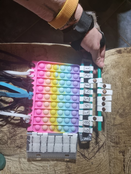
Text
Looks like a toy for playing around with some knot theory stuff
The numbers can be re-attached via velcro patches.
One can use the threads/shoelaces for playing with some weaving patterns. Additionally one can use the slilicone pop-up dots as a binary/boolean indicator, which might be a good helpful tool.
Due to material reasons this thing only has 9 columns. The number 0 might get a different place or calculation mechanism.
I also still do not really know how I really want to use this strange thing.
...
A well-working flap:

And a (useless) information for free:
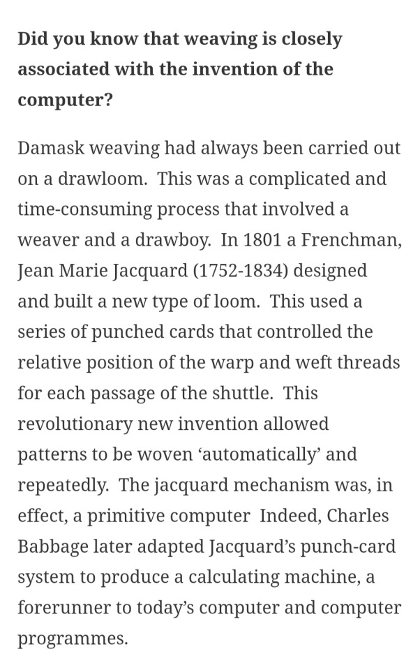
[ Source: lisburnmuseum.com ]
#kalkulationslappen 2.0#calculation rag#calculation rag 2.0#silly#semi-serious math#math#mathematics#mathposting#knot theory#knotty#knotty toy#mathy toy#autism intensifies#calc rag#whatever sort of non-trivial nonsense#threads#weaving#computer#cs#computer science#primitive computer#my strange silly crafts
85 notes
·
View notes
Text
First portion of an incomplete mathpost
I've tweeted a couple of times now that "forming a filterquotient is just taking the stalk of a stack". Let me explain what that means, for people who know what stalks, stacks, and elementary topoi are, but not filterquotients. You should probably also know what a filter is, though.
Before anything else, let me give a "direct" definition of what a filterquotient of a topos is, so that once the rest of the post works its way back around, you'll be able to see the equivalence. Let $\mathcal{E}$ be an elementary topos and $\Phi \subseteq \operatorname{Sub}(1)$ be a filter in the poset of subobjects of $\mathcal{E}$'s terminal object. For $U$ a subobject of $1$ and objects $X$, $Y$ we define the set $\operatorname{Hom}_U(X, Y)$ of "$U$-partial morphisms" from $X$ to $Y$ to be $\operatorname{Hom}(U \times X, Y)$; if $V \subseteq U$, then there is an evident "restriction map" from $\operatorname{Hom}_U(X, Y)$ to $\operatorname{Hom}_V(X, Y)$. We define the filterquotient $\mathcal{E}_\Phi$ to be the category with objects the same as those of $\mathcal{E}$ and where the hom-set from $X$ to $Y$ is $\varinjlim_{U \in \Phi} \operatorname{Hom}_U(X, Y)$, with composition given by composition in $\mathcal{E}$ on representatives. This new category will still be an elementary topos, although it need not be a Grothendieck topos even if $\mathcal{E}$ was one, and there is an evident functor $\mathcal{E} \to \mathcal{E}_\Phi$ which is a logical morphism. Exercise to understand this definition: Work out $\mathcal{E}_\Phi$ looks like in the case where $\mathcal{E}$ is $\mathrm{Set}^{\mathbb{N}}$ and $\Phi$ is the filter of cofinite subsets of $\mathbb{N}$.
Now we can work our way to seeing how this is a case of taking the stalk of a stack.
First of all, I'm using "stalk" in a slightly generalized sense, and I'm not completely sure whether any of its standard meanings actually apply literally to the case of filterquotients. To be a little more precise about the kind of generalization in question: traditionally, a stalk is something that you take of a sheaf and at a point, and while it's obvious that I'm generalizing along the first axis already by talking about stacks instead of just sheaves, I'm actually also generalizing along the second axis, by talking about stalks at filters instead of just stalks at points. Before I touch on filterquotients or stacks at all, let me begin by explaining what this latter generalization means.
The traditional first definition of a stalk goes something like this: you start with a space $X$, a sheaf $F$ on $X$ valued in some category $C$ of algebraic structures, and a point $p \in X$. Then you build the "stalk of $F$ at $p$" by first collecting all local sections of $F$ defined on all open neighborhoods of $p$, and then modding out by a "defines the same germ at $p$" relation. This is a very nuts-and-bolts definition that makes the content of the stalk very clear. However, it is not very categorypilled, which makes me sad. We can reformulate this definition to make it clear that the stalk is a certain colimit; this also allows generalization of the notion of stalk to [pre]sheaves valued in non-concrete categories. Let's be precise: let $N_p \subseteq O(X)$ be the collection of open neighborhoods of $p$, considered as a full subcategory of $O(X)$. Then we can restrict $F : O(X)^{\mathrm{op}} \to C$ to have domain $N_p^{\mathrm{op}}$. Considering this functor as a diagram in $C$ and taking its colimit, we get the stalk of $F$ at $p$.
The first thing to notice here is that we only use $p$ in order to form $N_p$. In particular, for any collection of opens $S \subseteq O(X)$, we can carry out the construction of restricting $F$ to have domain $S^{\mathrm{op}}$ and taking the colimit of the resulting diagram, so long as $C$ is cocomplete enough; nothing about these latter steps is reliant on us having an actual point in hand. The second thing to notice is that while we can do this for any collection of opens, $N_p$ does have some special properties that make taking stalks particularly nice. Most importantly, it is a filter in $O(X)$---it's called the "neighborhood filter" of $p$, to be precise. I actually can't speak off the top of my head to the significance, in this context, of the "upward closed" half of the definition of filters, but the "downward directed" half is crucial: it means that the category $N_p^{\mathrm{op}}$ is filtered, so that a colimit indexed by it is a filtered colimit. Filtered colimits are lovely for many reasons; one very very important one is that while a general colimit of algebraic structures need not be computed on the underlying sets as the same colimit---think of how a coproduct of groups is not computed on underlying sets as a coproduct of sets---a filtered colimit of algebraic structures is computed on underlying sets as the same colimit and then simply re-equipped with operations. Indeed, this is what allows the nuts-and-bolts description of stalks as a certain disjoint-union-and-quotient to work for sheaves valued in any category of algebraic structures, without needing to speak directly of abstract colimits. For this reason among others, I claim that being a filter is a desirable condition to impose on a collection of opens for it to be worth thinking about "stalks" there. So: given a sheaf (or presheaf) $F : O(X)^{\mathrm{op}} \to C$, for any filter $\Phi \subseteq O(X)$, let's call the colimit of the diagram $F|_{\Phi^{\mathrm{op}}}$ the stalk of $F$ at $\Phi$, or stalk of $F$ on $\Phi$. In the case that $C$ is a category of algebraic structures, this looks pretty much the same as usual, thanks to $\Phi$ being directed: we gather up all of the sections of $F$ on opens belonging to $\Phi$, then quotient by "agreeing on something in the intersection".
Now let me give two key sources of filters in $O(X)$ not of the form $N_p$ that are worth caring about, both to justify this generalization and to give an intuition for what it can look like.
We can form a neighborhood filter of any subset of $X$, not just of a point: if $A \subseteq X$ is any subset, not necessarily open or closed, let $N_A$ be the collection of opens that are supersets of $A$. This will always be a filter. This is a pretty natural object. For example, we can rephrase one classic result about paracompact spaces as follows: For any sheaf of sets, there is a map from the stalk on $N_A$ to the set of sections on $A$ of the étalé space, and for closed $A$ and paracompact $X$, this map is a surjection.
In many spaces, typically non-compact ones, we can form various filters of "neighborhoods of infinity" of one kind or another. Taking the stalk at such a filter gives us the "germs at infinity" of the corresponding kind. For example, if $X$ is the real line, we can let $\Phi$ be the collection of all opens which contain $(a, \infty)$ for some $a$. Then the stalk at $\Phi$ of, say, the sheaf of real-valued functions, really is the collection of germs at positive infinity.
(An aside on filters: In general, as in both of these examples, one can think of a filter as the collection of everything that contains a given point, or more generally, a given region. This makes it a kind of "formal intersection"; for example, a point is part of the region described by a filter (and we can evaluate germs on the filter at that point) iff it is an element of the literal intersection of all of the opens of the filter. However, the fact that the intersection is only formal means that a filter generally carries more information, and is a "larger region" than, the literal intersection of all of the opens in it. For example, the neighborhood filter of a point, or more generally a subset, can be seen as an "infinitesimal neighborhood" of that point or subset, while in a space satisfying mild separation axioms, the intersection of all of the opens in this filter is just the point or subset itself. And a filter of neighborhoods of infinity can be seen as a point at infinity, or really an infinitesimal neighborhood of such, while the intersection of all of the opens in such a filter is generally empty. In this view on filters, the stalk on a filter reveals itself as "local sections defined on the region described by the filter"; it is a colimit because we are taking a formal intersection (limit), passing it through a contravariant functor, and then evaluating.)
Much more generally than just the case of topological spaces, if $(D, J)$ is any site where $D$ is a poset, we can take the stalk of a sheaf on $(D, J)$ at a filter in $D$. We can generalize this further still, to non-poset sites, with a definition motivated by topos theory, but it will not be necessary for what I want to talk about and would require a pretty lengthy detour.
Having explained what it means to take a stalk at a filter, let me now talk about taking stalks of stacks. The definition that follows is just what seems to me to be what taking the stalk of a [pre]stack should clearly mean; I have not seen it in any sources. That said, I would not be surprised if it is out there, given that I haven't read a ton of stuff that uses stacks!
Consider a [pre]stack on a site $(D, J)$ in the form of a pseudofunctor $\mathcal{S} : D^{\mathrm{op}} \to \mathrm{Cat}$ (or more generally, we could consider stacks valued in a bicategory other than $\mathrm{Cat}$). If $D$ is a poset and $\Phi$ is a filter in $D$, then the same construction as above makes perfect sense: we have a cofiltered diagram in $D$ which we send through $\mathcal{S}$ to get a filtered diagram in $\mathrm{Cat}$. The stalk of $\mathcal{S}$ on $\Phi$ should be the 2-colimit of this filtered diagram. Filteredness allows us to give a pleasantly explicit formula for this 2-colimit for the case of values in $\mathrm{Cat}$, and for the case of values in any "concrete" bicategory where filtered 2-colimits are computed on underlying categories: The objects of $\mathcal{S}_\Phi$ are pairs $(d \in D, A \in \mathcal{S}(d))$, and the hom-sets are given by $\operatorname{Hom}((c, A), (d, B)) = \varinjlim_{e \leq c, d} \operatorname{Hom}(A|_e, B|_e)$. Composition is defined on representatives by... [TODO finish definition, double check, check coherence issues, justify the construction]
Let's do a simple example computation. Let $X$ be your favorite topological space, $\mathcal{S}$ be the stack of locally trivial real vector bundles on it (as a stack of groupoids), and $p$ be any point of $X$; we compute $\mathcal{S}_p$. We begin by establishing the connected components. Let $V_n = (X, X \times \mathbb{R}^n) \in \mathcal{S}_p$; I claim that every object of $\mathcal{S}_p$ is isomorphic to exactly one $V_n$. [TODO ...] Then, we establish the automorphism groups of each $V_n$. Since a pullback of a trivial bundle is trivial [TODO _fucking_ coherences] we have $\operatorname{Hom}(V_n, V_n) \cong \varinjlim_{p \in U} \operatorname{Hom}(U \times \mathbb{R}^n, U \times \mathbb{R}^n) \cong \varinjlim_{p \in U} \operatorname{Hom}(U, \operatorname{GL}(n))$. Of course, this is just the group of germs at $p$ of $\operatorname{GL}(n)$-valued functions.
Now we can start talking about which stack we're going to be taking a stalk of.
If $C$ is any category with pullbacks, there is a prestack on it of fundamental interest, called the "codomain fibration" when viewed as a category fibered in categories and the "self-indexing" when viewed as a contravariant pseudofunctor to $\mathrm{Cat}$. In its guise as the codomain fibration, it is $\operatorname{cod} : \operatorname{Arr}(C) \to C$. In its guise as the self-indexing, it is the pseudofunctor defined on objects by $S(A) = C/A$ and on morphisms by $S(f) = f^*$. For $C$ a Grothendieck topos, the self-indexing is in fact a stack with regard to the canonical topology on $C$---which, for a Grothendieck topos, is the one where coverings are families of morphisms such that the induced map from a coproduct is an epi. More generally, for $C$ an elementary topos (in fact, much weaker conditions suffice), the self-indexing is still a stack with respect to a "finitary" version of this topology, where the coverings are those finite families of morphisms such that the induced map from a coproduct is an epi. Finally, for the purposes we are interested in, we want to consider the restriction of the self-indexing to the poset of subobjects of $1$ (it is legitimate to call this "restriction" because this poset is equivalent to the full subcategory of $C$ on objects whose unique map to $1$ is monic). In the case of a Grothendieck topos, the resulting prestack continues to be a stack on this poset if we give it the Grothendieck topology where a family of elements covers another element just when that element is their sup (equivalently, is leq their sup). In the case of an elementary topos, arbitrary joins may not exist; but we will still be a stack for finite covering families.
As an example, let $X$ be a topological space and consider the Grothendieck topos $\operatorname{Sh}(X)$. Under the equivalence of $\operatorname{Sh}(X)$ with the category of étalé spaces over $X$, we can view the self-indexing of $\operatorname{Sh}(X)$ as a stack on that category instead. And given the pseudonatural-in-$F$ equivalence $\operatorname{Sh}(X)/F \simeq \operatorname{Sh}(\operatorname{Et}(F))$, we see that the resulting stack is the one which assigns each étalé space the category of sheaves on it. The terminal étalé space is $X$ itself; subobjects are just opens of $X$, so the subobject poset is $O(X)$, and the sup-based Grothendieck topology described above is the usual one on $O(X)$, so the restricted stack is a stack on $X$ in the usual sense. In particular, it is the stack $U \mapsto \operatorname{Sh}(U)$.
Finally, we can put the pieces together!
magic katex-enabling link
1 note
·
View note
Text
If you’re curious to why I really don’t like numerics, consider the following paradox.
Theorem: Any system of arrows can be taken as a binary operator if you remember that, in the system where it behaves like an operator, it is binary.
Given the concept of binary operators, if you can take anything as a binary operator, you can also take any unary operator as a binary operator. For every unary operation, there is an interpretation in which it is seen as a binary operator:
If u’m serious (but that’s not a typo): Two equals a (2) + a (3) + a (1) + a (5) = 2(5) + 2(4) + 2(3) = 5(5) + 3(4) + 3(2) = 12 = 15(5) = 20 = 20(8) = 20 (2)
When you take the exponent as a binary operation, you’ll just think of it as 2.
Sometimes when I was young I thought it was supposed to be 2 because I was in 3/2 time. But the basic concept is the same.
I think the above is a good example of where some numbers aren’t meant to be binary, except by doing arbitrary silly things to one or more of them.
For a while I thought that 2/3 time was also like a binary operator, but no one outside of me would understand me. I thought they meant 3/3 time.
I also thought that, because I was in 3/2 time, you could compute anything by adding two 3/2 times and placing the result in the right column, and also that you could multiply by (only) multiplying by 3/2.
The trick to interpreting any number as a binary operator (which you can definitely do) involves taking the answer and placing it in the right column. So that it makes sense.
There’s a bunch of dumb reasons for thinking the operators should be binary (because the double.number method has to resort to putting a null in two boxes or else no terminal.’).
But consider, if you’re in 3/2 time, (What your choice of path through the timeline is gonna be. [Non-tenuous train of thought])
Path A is: A, B, C, D, C, C, D, D.
Path B is: B, A, B, D.
Path C is: B, A, C, D.
And what’s it gonna be? (Is just about a possible A vs. A)
Path D is the next choice, which may be: A, C, B, A, B.
So you go through A to C to go D.
“And A is B.”
I guess people think the operators should be all of them besides A and A.
I can’t think of an argument for “#mathpost<|
2 notes
·
View notes
Text
i wonder what the statistics of my blog theme breakdown is. like how much of it is shitposting, versus mathposting, versus like, random fandom shit
i guess there's a good amount of politics and non-shit-comedy posting as well. art? do i post art? i think so??? i DEFINITELY post short stories, somethimes. hm.
0 notes
Text
Connecting two notions of orientation on manifolds
Mathpost incoming. I mentioned in my last post that LaTeX, although convenient, only reads well on my actual blog’s page, not the dashboard. So I will be using images from now on after this post probably. If you want to see this post how it’s meant to be, check out the blog. Anyways...
So, I was reading “Introduction to 3-Manifolds” by Jennifer Schultens and I noticed she defined orientation on manifolds in a different way than Hatcher does in his “Algebraic Topology”. Hatcher defines an “orientation” as a mapping $x\rightarrow{\mu_{x}}$ for $x\in{M}$, where $\mu_{x}$ is a local orientation in $H_{n}(M,M\setminus{x})$ such that each $x$ has an nhood containing a finite radius open ball $\mathbb{B}_{\epsilon}$ about $x$ such that all local orientation $\mu_{y}$ for $y\in{\mathbb{B}_{\epsilon}}$ are in the images of a generator $\mu_{\mathbb{B}}$ in $H_{n}(M,M\setminus{\mathbb{B}_{\epsilon}})$, under natural maps $H_{n}(M,M\setminus{\mathbb{B}_{\epsilon}})\rightarrow{H_{n}(M,M\setminus{y})}$.
...Okay, that fine, but then Shultens defines an orientable smooth manifold as: a manifold $M$ that has an atlas such that all of the Jacobians of the transition maps have positive determinant.
...How are they related? Turns out, there’s lots of literature on the topic online, so I’ll just talk about this here. Well, we note that the homological definition works for general manifolds, not necessarily smooth ones, so we’d want to only see how the homological definition (I’ll call this HomDef) implies the smooth Jacobian definition (I’ll call this SmDef) on smooth manifolds. We want:
(HomDef $\rightarrow$ SmDef)
...Note that we’re dealing with relative homology groups of the form $H_{n}(M,M\setminus{x})$, intuitively, these are the homology groups on the relative chain complex where each relative chain group ignores all the chains that don’t contain the point $x$, so:
...where everything is in our manifold $M$. Now then, let’s assume $M$ is a smooth manifold with the HomDef of orientable. Also, we need to choose an orientation for $\mathbb{R}^{n}$, we’ll do this by selecting a generator for the relative homology group $H_{n}(\mathbb{R}^{n},\mathbb{R}^{n}\setminus{\{0\}})$. Since $M$ is a smooth manifold, let it have an atlas $\{M_{\alpha},\phi_{\alpha}\}$, where each $\phi_{\alpha}$ is a diffeomorphism sending $M_{\alpha}$ to an open subset of $\mathbb{R}^{n}$. Recall then the following theorem:
$\textbf{Excision Theorem:}$ Given subspaces $Z\subset{A}\subset{X}$ where $\bar{Z}$ ($Z$’s closure) is contained in $Int{A}$, then the inclusion $(X-Z,A-Z)\rightarrow{(X,A)}$ induces an isomorphisms of homology groups $H_{n}(X\setminus{Z},A\setminus{Z})\rightarrow{H_{n}(X,A)}$ for all $n$.
...Excision implies that the map induced by the inclusion $i:(U_{\alpha},U_{\alpha}\setminus{x})\rightarrow{(M,M\setminus{x})}$ is an isomorphism on homology groups. Also, noting that $\phi_{\alpha}$ is a diffeomorphism and therefore a homeomorphism, we have the following isomorphisms:
$H_{n}(M,M\setminus{x})\equiv{H_{n}(U_{\alpha},U_{\alpha}}\setminus{x})\equiv{H_{n}(\mathbb{R}^{n},\mathbb{R}^{n}\setminus{\{0\}})}$
...we then need one more lemma for this all to make sense:
$\textbf{Lemma:}$ Given a diffeomorphism $\Phi:(\mathbb{R}^{n},0)\rightarrow{(\mathbb{R}^{n},0)}$, the induced maps on $H_{n}(\mathbb{R}^{n},\mathbb{R}^{n}\setminus{\{0\}}$ leave generators alone if and only if the Jacobian’s determinant of $\Phi$ at 0 is positive.
Thus, also noting that smooth maps $\mathbb{R}^{n}\rightarrow{\mathbb{R}^{n}}$ are homotopic to the Jacobian at 0, and the $n\times{n}$ general linear group over $\mathbb{R}$ has two connected components, each determined by the sign of the $\det$ function (clearly, as the elements of $GL_{n}(\mathbb{R})$ have non-zero determinant, so the range of $\det$ here is $(-\infty,0)\cup{(0,\infty)}$), thus, the induced map on homology groups $H_{n}(\mathbb{R}^{n},\mathbb{R}^{n}\setminus{\{0\}})$ is just the sign of the Jacobian of the smooth map $f:(\mathbb{R}^{n})\rightarrow{(\mathbb{R}^{n},0)}$ at 0. Thus, if the charts have correct homological orientation, then by the lemma and above the transition maps will have positive Jacobian determinant.
...So, to summarize, diffeomorphisms preserve the generator of the homology groups iff the Jacobian determinant is positive. Smooth maps fixing 0 are homotopic to the Jacobian of that smooth function at 0. $GL_{n}(\mathbb{R})$ has two connected components, determined by determinant, so the induced by $f$ on homology is the sign of the Jacobian determinant of $f$ at 0, implying that, choosing charts following the HomDef implies the SmDef.
...To prove (SmDef $\rightarrow$ HomDef) for smooth manifolds, the same argument above works, we are just choosing a generator for $H_{n}(M,M\setminus{x})$ by an oriented chart.
...Okay that’s it. I basically followed the post(s) linked below for this. Just wanted to understand this bit of math better, now I do. Bye!
__________________________________________
Sources:
- https://math.stackexchange.com/questions/2878579/homological-orientation-vs-smooth-orientation
-https://math.stackexchange.com/questions/43779/equivalent-definitions-of-orientation?rq=1
-”Algebraic Topology” -A. Hatcher
-”Introduction to 3-manifolds” -J. Schultens
0 notes