#process lasso activation code | Explore Tumblr posts and blogs

disasterbijamietartt · 2 years ago

Text

I’ll need a few days to really process the last episode, so don’t expect any meta until the weekend.

But I wanted to write a post about why I believe in the writers and why I think that … this sounds so arrogant and delusional, but that my predictions here* are roughly what will happen and queer folks can stay hopeful.

(*tl;dr: Essentially that Colin will be the inspiration for main characters to address their queerness, Ted Lasso spent two seasons straightbaiting its entire audience and this season will end queer as fuck)

When I started watching Ted Lasso I thought it would be a fun, but silly little sports comedy, but very soon it got obvious how the show featured heavier themes and that they didn’t follow the expected script. Like, when Rebecca tells Ted the truth, you’d normally get some drama and rising conflict – but we got instant forgiveness.

And it got soon obvious we’d get a love triangle with Jamie, Keeley and Roy and – as someone who knows how the script goes – my first assumption was, that Roy x Keeley will be endgame (which was sad, since I adored Jamie x Keeley from the beginning, but I digress).

But some of the things that usually put me off love triangles were missing: there was no prolonged unnecessary drama after Roy learned that Keeley hooked up with Jamie the night before, Jamie and Roy didn’t fight over who would “get” Keeley (even though Roy’s jealousy sure was one reason for the tension between him and Jamie, but it wasn’t the only one), Jamie didn’t try to actively win Keeley back throughout the second season, he didn’t try to sabotage their relationship, even though he still loved her. The rocky parts in Roy’s and Keeley’s relationship weren’t related to Jamie at all, on the contrary, Jamie kind of unintentionally fixed their problems.

So, when they diverge so much from the expected, should I really still assume they’ll end the show with the thing everyone expects to happen? (like, in classic romance structure, Roy and Keeley now had their third act break-up, that always happens before the happily ever after … but as Phil said in an interview, they’re situation is a lot more complex than you’ll usually get.)

So, anyway, Ted Lasso was playing with expectations from the beginning. You’d expect Ted x Rebecca and Roy x Keeley endgame cause that is how the classic narrative works but the show subverted classic structure in the first season. So why should we assume that they just stick to the classic script now?

Also the theme song:

“Yeah, might be all that you get,

Yeah, I guess this might well be it“

I always thought, for an optimistic show like Ted Lasso this was a kinda sober beginning. But if you look at this with a queer eye … Cishet people are so used to seeing their happy endings playing out, so that is what they’ll expect to get. Until the last couple years, queer people barely got any stories with happy endings, so you didn’t exactly grow up with the expectation you’ll get a happy ending.

So you just had to take what you got.

But on the other hand the song has this hopeful bit about trying and not giving up. And … okay, I’m not sure where I’m going with this, but, idk, it just feels like it would fit as the theme song for an ultimately hella queer show?

And there are a lot of allusions to “The Wizard of Oz”, starting with the title of the first episode, Ted being the “Man from Kansas” aka Dorothy – googling I found this post pointing out a lot parallels in the second season, so it is not just me being delusional again.

For context: The movie was released 1939. Between 1934 and 1968 due to the Hays Code people couldn’t be shown as being explicitly queer in movies in the US, so writers started to queercode characters to still indicate queerness. And there is of course queercoding in “The Wizard of Oz” just like Ted Lasso and the movie as a whole resonated a lot with queer audiences, making Judy Garland a Gay Icon (see here).

Both the movie and L. Frank Baumans novels have a lot of queer subtext (like, there is even kind of a trans character in the novels?). "Friend of Dorothy” was a way gay men referred to each other at a time, where they couldn’t just openly ask about someone’s orientation.

Fun Fact: The movies title song “Over the Rainbow” soon became a queer anthem and people wondered whether it inspired the rainbow flag. But the creator, Gilbert Baker, said he was inspired by,

wait for it,

“She’s a Rainbow” by the Rolling Stones (see here).

Rings a bell?

The episode “Rainbow”?

Roy returning as a coach to Richmond?

Also: Jamie comparing the team to the Rolling Stones? Himself to Mick Jagger and Roy to Keith Richards, who both wrote the song?

And, looking at episode titles some more: The color "Lavender" is so queer it has it's own LGTBQ-section on Wikipedia. Also the bisexual pride flag, where the colours overlap to form lavender? There was probably some other reason I forgot that the episode where Jamie returned was called like the queerest color ever, but still …

WHAT A BUNCH OF CURIOUS COINCIDENCES!

Oh God, the more I look, the queerer everything gets! I think I could go on some more, but I need to get breakfast and then some work done.

#my meta #ted lasso speculations #jamie x roy #roy x jamie #ted x trent #tedtrent #tedependent #colin hughes #jamie x keeley x roy #this doesn't reference any ship but might be relevant soo #if I'm wrong I delete my tumblr #and burn something down #kidding I'll just never trust a tv show ever again #ted lasso meta #queer coding #ted lasso

110 notes · View notes

hitplugins · 5 years ago

Link

Process Lasso Pro 9.9.1.23 With Activation Code Full Version Crack Lasso Process Crack Key is a Windows process automation and optimization software. From optimization algorithms like ProBalance to user-generated rules and persistent settings like CPU affinity and priority class, Process Lasso lets you take full control over the running apps! The Process Lasso Pro Free...

#Process Lasso Pro Crack #Process Lasso Pro Activation Code #Process Lasso Pro Key

0 notes

nanncyy-blog1 · 6 years ago

Link

#process lasso pro 9 crack #process lasso pro activation code #process lasso pro crack

0 notes

agenlioolindaa-blog · 6 years ago

Link

#process lasso pro 9 crack #process lasso pro activation code #process lasso pro crack

0 notes

shari-1-blog · 6 years ago

Text

Bitsum Process Lasso Pro Crack Full Keygen

Bitsum Process Lasso Pro 9.3.0.74 Crack Full Keygen

Process Lasso Crack also gives a variety of methods to fully control how the CPU ways assigned to a running program. You can select which priority processes should executes and which CPUs (cores) should assigns to them. So, You can also disable certain tools, register all executed softwares, and more (see the list below).

Process Lasso…

View On WordPress

#Bitsum Process Lasso #Bitsum Process Lasso Crack #Process Lasso #Process Lasso Activation Code #Process Lasso Crack #Process Lasso License Key #Process Lasso Pro #Process Lasso Pro Crack #Process Lasso Serial Key

0 notes

zhanariem · 2 years ago

Text

Week 3: Running a Lasso Regression Analysis

Warning ¡Change this line, deprecated code!

from sklearn.cross_validation import train_test_split

from sklearn.model_selection import train_test_split

Running in Linux Ubuntu

Installation in Linux Ubuntu.

sudo chmod +x Anaconda3-2022.10-Linux-x86_64.sh

./Anaconda3-2022.10-Linux-x86_64.sh

conda install scikit-learn

conda install -n my_environment scikit-learn

pip install sklearn

pip install -U scikit-learn scipy matplotlib

sudo apt-get install graphviz

sudo apt-get install pydotplus

conda create -c conda-forge -n spyder-env spyder numpy scipy pandas matplotlib sympy cython

conda create -c conda-forge -n spyder-env spyder

conda activate spyder-env

conda config --env --add channels conda-forge

conda config --env --set channel_priority strict

python -m pip install pydotplus

All predictor variables were standardized to have a mean of zero and a standard deviation of one.

Data were randomly split into a training set that included 70% of the observations (N=3201) and a test set that included 30% of the observations (N=1701). The least angle regression algorithm with k=10 fold cross validation was used to estimate the lasso regression model in the training set, and the model was validated using the test set. The change in the cross validation average (mean) squared error at each step was used to identify the best subset of predictor variables.

During the estimation process, self-esteem and depression were most strongly associated with school connectedness, followed by engaging in violent behavior and GPA. Depression and violent behavior were negatively associated with school connectedness and self-esteem and GPA were positively associated with school connectedness. Other predictors associated with greater school connectedness included older age, Hispanic and Asian ethnicity, family connectedness, and parental involvement in activities. Other predictors associated with lower school connectedness included being male, Black and Native American ethnicity, alcohol, marijuana, and cocaine use, availability of cigarettes at home, deviant behavior, and history of being expelled from school. These 18 variables accounted for 33.4% of the variance in the school connectedness response variable.

0 notes

waressoftpc · 4 years ago

Link

#Process Lasso Pro 10

0 notes

archanawathore · 4 years ago

Text

Machine Learning Assignment 3

ML_Assignment3

SAS Code:

libname mydata "/courses/d1406ae5ba27fe300" access=readonly;

**************************************************************************************************************

DATA MANAGEMENT

**************************************************************************************************************;

data new;

set mydata.treeaddhealth;;

if bio_sex=1 then male=1;

if bio_sex=2 then male=0;

* delete observations with missing data;

if cmiss(of _all_) then delete;

run;

ods graphics on;

* Split data randomly into test and training data;

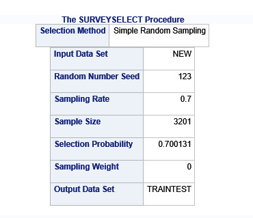
proc surveyselect data=new out=traintest seed = 123

samprate=0.7 method=srs outall;

run;

* lasso multiple regression with lars algorithm k=10 fold validation;

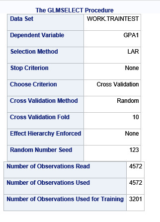
proc glmselect data=traintest plots=all seed=123;

partition ROLE=selected(train='1' test='0');

model gpa1 = male hispanic white black namerican asian alcevr1 marever1 cocever1

inhever1 cigavail passist expel1 age alcprobs1 deviant1 viol1 dep1 esteem1 parpres paractv

famconct schconn1/selection=lar(choose=cv stop=none) cvmethod=random(10);

run;

Explanation

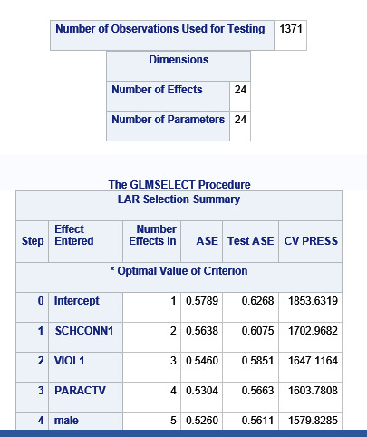
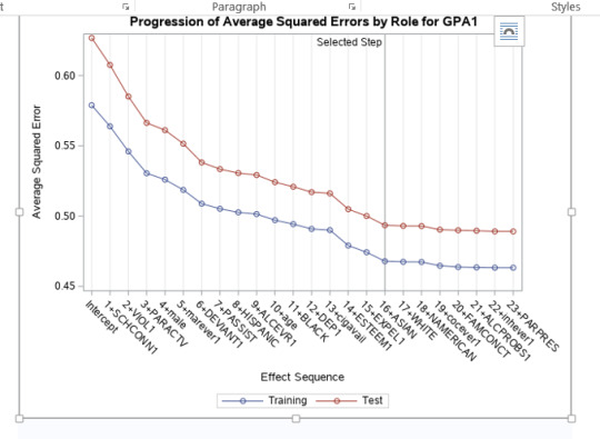
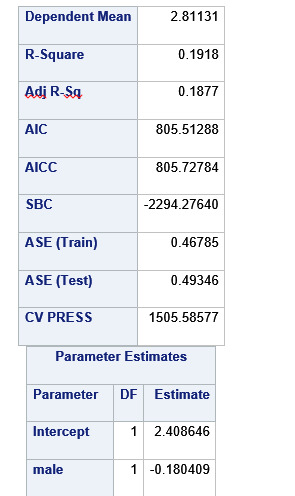
A lasso regression analysis was conducted to identify a subset of variables from a pool of 23 categorical and quantitative predictor variables that best predicted a quantitative response variable measuring grade point average in adolescents. Categorical predictors included gender and a series of 5 binary categorical variables for race and ethnicity (Hispanic, White, Black, Native American and Asian). Binary substance use variables were measured with individual questions about whether the adolescent had ever used alcohol, marijuana, cocaine or inhalants. Additional categorical variables included the availability of cigarettes in the home, whether or not either parent was on public assistance and any experience with being expelled from school. Quantitative predictor variables include age, school connectedness, alcohol problems, and a measure of deviance that included such behaviors as vandalism, other property damage, lying, stealing, running away, driving without permission, selling drugs, and skipping school. Another scale for violence, one for depression, and others measuring self-esteem, parental presence, parental activities, family connectedness and were also included. All predictor variables were standardized to have a mean of zero and a standard deviation of one.

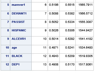
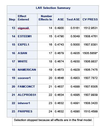
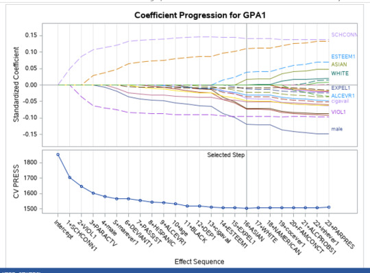
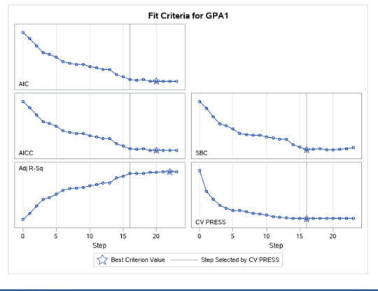
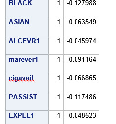
During the estimation process, school connectedness and violent behavior were most strongly associated with grade point average, followed by parental activities and male. Being male and violent behavior were negatively associated with grade point average, and school connectedness and parental activities were positively associated with grade point average. Other predictors associated with greater gpa included self esteem, Asian and White ethnicity, family connectedness, and parental involvement in activities. Other predictors associated with lower gpa included being Black and Hispanic ethnicities, age, alcohol, marijuana use, depression, availability of cigarettes at home, deviant behavior, parent was on public assistance, and history of being expelled from school. These 16 variables were selected for grade point average response variable. Ethnicity ASIAN was selected as best model.

Result

0 notes

happycloudwolf · 4 years ago

Link

Process Lasso 10.0.0.164 Serial key is software for setting the priority of the running process, monitor RAM, and also manage active applications

0 notes

taimoorrafique · 4 years ago

Text

Process Lasso Pro 9.8.7.18 Crack + Key Download [Latest]

Process Lasso Pro Crack Free Download is a professional version of a small utility that allows you to manually or automatically manipulate the running on your computer for maximum speed and stability. This utility is not a replacement for the standard process manager; rather, it adds new features that allow you to optimize CPU performance at maximum load.

Process Lasso Pro Activation Code Download allows you to determine the priority of Process Lasso Pro Key, and, at the request of the user, the priority will be set for all subsequent launches. Process Lasso Pro License Key is a unique new technology that will, amongst other things, improve your PCs responsiveness and stability.

Windows, by design, allows programs to monopolize your CPU without restraint – leading to freezes and hangs. Process Lasso Pro Serial Key 2021 (Process Balance) technology intelligently adjusts the priority of running programs so that badly behaved or overly active processes won’t interfere with your ability to use the computer.

Process Lasso Pro Key Features:

Unique Process Lasso Pro 9 Key technology safely and effectively improves PC responsiveness!

Max performance when active, but conserve energy when the PC is idle!

Automate & control process priorities, CPU affinities, power plans and more!

Activate the Bitsum Highest Performance power plan for max performance.

Localized to: English, German, French, Polish, Finnish, Italian, PTBR, Russian, Japanese, Chinese.

Ensures optimal performance at all times for real-time applications!

Native 64-bit code for maximum performance on Workstations and Servers!

Supports Windows XP to Windows 10, and all Server Variants (Server Edition only).

We are not a fan of RAM optimization, so created a SAFE and CONSERVATIVE algorithm for those who do need such.

How to Crack or Activate Process Lasso Pro 9.8.7.18 Keygen??

First download from the given link or button.

Uninstall the Previous version with IObit Uninstaller Pro

Turn off the Virus Guard.

Then extract the rar file and open the folder (Use Winrar or Winzip to extract).

Run the setup and close it from everywhere.

Open the “Crack” or “Patch” folder, copy and paste into installation folder and run.

Or use the serial key to activate the Program.

All done enjoy.

Also Download

WinRAR Crack 32/64-bit License Key Full [Latest 2021]

IDM Crack 6.38 Build 16 Keygen With Torrent Download (2021)

Ant Download Manager Pro Crack + Registration Key [Latest]

IOBIT Uninstaller Pro Crack + Serial Key Full (Updated 2021)

0 notes

ggonecrane-ml4daprojects · 4 years ago

Text

Week 3 Assignment - Running a Lasso Regression Analysis

Introduction

In this assignment I am going to perform a Lasso Regression analysis using k-fold cross validation to identify a subset of predictors from 24 or so of predictor variables that best predicts my response variable. My data set is from Add Health Survey, Wave 1.

My response variable is students’ academic performance in the measurement of students grade point average, labelled as GPA1, in which 4.0 is the maximum value.

The predictor variables I have used for this analysis are as follows:

Data Management

Since my original raw dataset contains quite a few missing values in some columns and rows, I have created a new dataset by removing any rows with missing data via Pandas’ dropna() function. Also, I have managed BIO_SEX variable by re-coding its female value to 0 and male value to 1, and called it a new variable MALE.

Program

My Python source for this analysis is appended at the bottom of this report.

Analysis

In this analysis, I have programmed to randomly split my dataset into a training dataset consisting of 70% of the total observations and a test dataset consisting of the other 30% of the observations. In terms of model selection algorithm, I have used Least Angle Regression (LAR) algorithm.

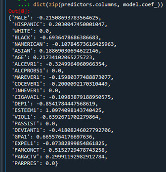
First, I have run k-fold cross-validation with k =10, meaning 10 random folds from the training dataset to choose the final statistical model. The following is the list of coefficient values obtained:

-------------------------------------------------------------------------------------

Coefficient Table (Sorted by Absolute Value)

-------------------------------------------------------------------------------------

{'WHITE': 0.0,

'INHEVER1': 0.0002990082208926463,

'PARPRES': -0.002527493803234668,

'FAMCONCT': -0.009013886132829411,

'EXPEL1': -0.009800613179381865,

'NAMERICAN': -0.011971527818286374,

'DEP1': -0.013819592163450321,

'COCEVER1': -0.016004694549008488,

'ASIAN': 0.019825632747609248,

'ALCPROBS1': 0.026109998722006623,

'ALCEVR1': -0.030053393438026644,

'DEVIANT1': -0.03398238436410221,

'ESTEEM1': 0.03791720034719747,

'PASSIST': -0.041636965715495806,

'AGE': -0.04199151644577515,

'CIGAVAIL': -0.04530490276829347,

'HISPANIC': -0.04638996070701919,

'MAREVER1': -0.06950247134179253,

'VIOL1': -0.07079177062520403,

'BLACK': -0.08033742139890393,

'PARACTV': 0.08546097579217665,

'MALE': -0.108287101884112,

'SCHCONN1': 0.11836667293459634}

As the result shows, there was one predictor at the top, WHITE ethnicity, of that regression coefficient shrunk to zero after applying the LASSO regression penalty. Hence, WHITE predictor would not be made to the list of predictors in the final selection model. Among the predictors made to the list though, the last five predictors turned out to be the most influential ones: SCHCONN1, MALE, PARACTV, BLACK, and VIOL1.

SCHCONN1 (School connectedness) and PARACTV (Activities with parents family) show the largest regression coefficients, 0.118 and 0.085, respectively. They apparently are strongly positively associated with students GPA. MALE (Gender), BLACK (Ethnicity), and VIOL1 (Violence) however, coefficients of -0.108, -0.080, and -0.070, respectively, are the ones strongly negatively associated with students GPA.

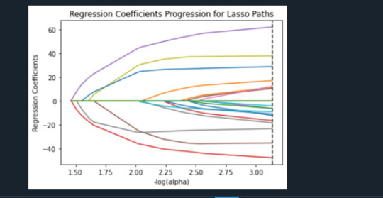
The following Lasso Path plot depicts such observations graphically:

The plot above shows the relative importance of the predictor selected at any step of the selection process, how the regression coefficients changed with the addition of a new predictor at each step, as well as the steps at which each variable entered the model. As we already saw in the list of the regression coefficients table above, two of positive strongest predictors are paths, started from low x-axis, with green and blue color, SCHCONN1 and PARACTV, respectively. Three of negative strongest predictors are the ones, started from low x-axis, drawn downward as the alpha value on the x-axis increases, with brown (MALE), grey (BLACK), and cyan (VIOL1) colors, respectively.

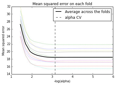
The following plot shows mean square error on each fold:

We can see that there is variability across the individual cross-validation folds in the training data set, but the change in the mean square error as variables are added to the model follows the same pattern for each fold. Initially it decreases rapidly and then levels off to a point at which adding more predictors doesn't lead to much reduction in the mean square error.

The following is the average mean square error on the training and test dataset.

-------------------------------------------------------------------------------------

Training Data Mean Square Error

-------------------------------------------------------------------------------------

0.4785435409557714

-------------------------------------------------------------------------------------

Test Data Mean Square Error

-------------------------------------------------------------------------------------

0.44960217328334645

As expected, the selected model was less accurate in predicting students GPA in the test data, but the test mean square error was pretty close to the training mean square error. This suggests that prediction accuracy was pretty stable across the two data sets.

The following is the R square for the proportion of variance in students GPA:

-------------------------------------------------------------------------------------

Training Data R-Square

-------------------------------------------------------------------------------------

0.20331942870725228

-------------------------------------------------------------------------------------

Test Data R-Square

-------------------------------------------------------------------------------------

0.2183030945000226

The R-square values were 0.20 and 0.21, indicating that the selected model explained 20 and 21% of the variance in students GPA for the training and test sets, respectively.

======== Program Source Begin =======

#!/usr/bin/env python3 # -*- coding: utf-8 -*- """ Created on Fri Feb 5 06:54:43 2021

@author: ggonecrane """

#from pandas import Series, DataFrame import pandas as pd import numpy as np import matplotlib.pylab as plt from sklearn.model_selection import train_test_split from sklearn.linear_model import LassoLarsCV import pprint

def printTableLabel(label): print('\n') print('-------------------------------------------------------------------------------------') print(f'\t\t\t\t{label}') print('-------------------------------------------------------------------------------------')

#Load the dataset data = pd.read_csv("tree_addhealth.csv")

#upper-case all DataFrame column names data.columns = map(str.upper, data.columns)

# Data Management recode1 = {1:1, 2:0} data['MALE']= data['BIO_SEX'].map(recode1) data_clean = data.dropna()

resp_var = 'GPA1' # 'SCHCONN1' # exp_vars = ['MALE','HISPANIC','WHITE','BLACK','NAMERICAN','ASIAN', 'AGE','ALCEVR1','ALCPROBS1','MAREVER1','COCEVER1','INHEVER1','CIGAVAIL','DEP1', 'ESTEEM1','VIOL1','PASSIST','DEVIANT1','GPA1','EXPEL1','FAMCONCT','PARACTV', 'PARPRES','SCHCONN1'] exp_vars.remove(resp_var)

#select predictor variables and target variable as separate data sets predvar= data_clean[exp_vars]

target = data_clean[resp_var]

# standardize predictors to have mean=0 and sd=1* predictors=predvar.copy() from sklearn import preprocessing

for key in exp_vars: predictors[key]=preprocessing.scale(predictors[key].astype('float64'))

# split data into train and test sets pred_train, pred_test, tar_train, tar_test = train_test_split(predictors, target, test_size=.3, random_state=123)

# specify the lasso regression model model=LassoLarsCV(cv=10, precompute=False).fit(pred_train,tar_train)

# print variable names and regression coefficients res_dict = dict(zip(predictors.columns, model.coef_)) pred_dict = dict(sorted(res_dict.items(), key=lambda x: abs(x[1]))) printTableLabel('Coefficient Table (Sorted by Absolute Value)') pprint.pp(pred_dict)

# plot coefficient progression m_log_alphas = -np.log10(model.alphas_) ax = plt.gca() plt.plot(m_log_alphas, model.coef_path_.T) plt.axvline(-np.log10(model.alpha_), linestyle='--', color='k', label='alpha CV') plt.ylabel('Regression Coefficients') plt.xlabel('-log(alpha)') plt.title('Regression Coefficients Progression for Lasso Paths')

# plot mean square error for each fold m_log_alphascv = -np.log10(model.cv_alphas_) plt.figure() plt.plot(m_log_alphascv, model.mse_path_, ':') plt.plot(m_log_alphascv, model.mse_path_.mean(axis=-1), 'k', label='Average across the folds', linewidth=2) plt.axvline(-np.log10(model.alpha_), linestyle='--', color='k', label='alpha CV') plt.legend() plt.xlabel('-log(alpha)') plt.ylabel('Mean squared error') plt.title('Mean squared error on each fold')

# MSE from training and test data from sklearn.metrics import mean_squared_error train_error = mean_squared_error(tar_train, model.predict(pred_train)) test_error = mean_squared_error(tar_test, model.predict(pred_test)) printTableLabel('Training Data Mean Square Error') print(train_error) printTableLabel('Test Data Mean Square Error') print(test_error)

# R-square from training and test data rsquared_train=model.score(pred_train,tar_train) rsquared_test=model.score(pred_test,tar_test) printTableLabel('Training Data R-Square ') print(rsquared_train) printTableLabel('Test Data R-Square ') print(rsquared_test)

======== Program Source End =======

0 notes

warez4wins · 4 years ago

Link

0 notes

lassoregression-blog1 · 5 years ago

Text

Lasso Regression

A lasso regression analysis was conducted to identify a subset of variables from categorical and quantitative predictor variables that best predicted a quantitative response variable measuring school connectedness in adolescents. Categorical predictors included gender and a series of 5 binary categorical variables for race and ethnicity (Hispanic, White, Black, Native American and Asian) to improve interpretability of the selected model with fewer predictors. Binary substance use variables were measured with individual questions about whether the adolescent had ever used alcohol, marijuana, cocaine or inhalants. Additional categorical variables included the availability of cigarettes in the home, whether or not either parent was on public assistance and any experience with being expelled from school. Quantitative predictor variables include age, alcohol problems, and a measure of deviance that included such behaviors as vandalism, other property damage, lying, stealing, running away, driving without permission, selling drugs, and skipping school. Another scale for violence, one for depression, and others measuring self-esteem, parental presence, parental activities, family connectedness and grade point average were also included. All predictor variables were standardized to have a mean of zero and a standard deviation of one.

The steps are-

1) Importing dataset – Here we load the dataset from the computer.

AH_data = pd.read_csv("tree_addhealth.csv")

2) Clean and manage the data

data_clean = data.dropna()

recode1 = {1:1, 2:0}

data_clean['MALE']= data_clean['BIO_SEX'].map(recode1)

3) select predictor variables and target variable as separate data sets.

predvar= data_clean[['MALE','HISPANIC','WHITE','BLACK','NAMERICAN','ASIAN',

'AGE','ALCEVR1','ALCPROBS1','MAREVER1','COCEVER1','INHEVER1','CIGAVAIL','DEP1',

'ESTEEM1','VIOL1','PASSIST','DEVIANT1','GPA1','EXPEL1','FAMCONCT','PARACTV',

'PARPRES']]

4) standardize predictors to have mean=0 and sd=1

predictors=predvar.copy()

from sklearn import preprocessing

predictors['MALE']=preprocessing.scale(predictors['MALE'].astype('float64'))

predictors['HISPANIC']=preprocessing.scale(predictors['HISPANIC'].astype('float64'))

predictors['WHITE']=preprocessing.scale(predictors['WHITE'].astype('float64'))

predictors['NAMERICAN']=preprocessing.scale(predictors['NAMERICAN'].astype('float64'))

predictors['ASIAN']=preprocessing.scale(predictors['ASIAN'].astype('float64'))

predictors['AGE']=preprocessing.scale(predictors['AGE'].astype('float64'))

predictors['ALCEVR1']=preprocessing.scale(predictors['ALCEVR1'].astype('float64'))

predictors['ALCPROBS1']=preprocessing.scale(predictors['ALCPROBS1'].astype('float64'))

predictors['MAREVER1']=preprocessing.scale(predictors['MAREVER1'].astype('float64'))

predictors['COCEVER1']=preprocessing.scale(predictors['COCEVER1'].astype('float64'))

predictors['INHEVER1']=preprocessing.scale(predictors['INHEVER1'].astype('float64'))

predictors['CIGAVAIL']=preprocessing.scale(predictors['CIGAVAIL'].astype('float64'))

predictors['DEP1']=preprocessing.scale(predictors['DEP1'].astype('float64'))

predictors['ESTEEM1']=preprocessing.scale(predictors['ESTEEM1'].astype('float64'))

predictors['VIOL1']=preprocessing.scale(predictors['VIOL1'].astype('float64'))

predictors['PASSIST']=preprocessing.scale(predictors['PASSIST'].astype('float64'))

predictors['DEVIANT1']=preprocessing.scale(predictors['DEVIANT1'].astype('float64'))

predictors['GPA1']=preprocessing.scale(predictors['GPA1'].astype('float64'))

predictors['EXPEL1']=preprocessing.scale(predictors['EXPEL1'].astype('float64'))

predictors['FAMCONCT']=preprocessing.scale(predictors['FAMCONCT'].astype('float64'))

predictors['PARACTV']=preprocessing.scale(predictors['PARACTV'].astype('float64'))

predictors['PARPRES']=preprocessing.scale(predictors['PARPRES'].astype('float64'))

5) split data into train and test sets.

pred_train, pred_test, tar_train, tar_test = train_test_split(predictors, target, test_size=.3, random_state=123)

6) Now we need to specify the lasso regression model.

model=LassoLarsCV(cv=10, precompute=False).fit(pred_train,tar_train)

7) plot coefficient progression

m_log_alphas = -np.log10(model.alphas_)

ax = plt.gca()

plt.plot(m_log_alphas, model.coef_path_.T)

plt.axvline(-np.log10(model.alpha_), linestyle='--', color='k', label='alpha CV')

plt.ylabel('Regression Coefficients')

plt.xlabel('-log(alpha)')

plt.title('Regression Coefficients Progression for Lasso Paths')

8) plot mean square error for each fold

m_log_alphascv = -np.log10(model.cv_alphas_)

plt.figure()

plt.plot(m_log_alphascv, model.cv-mse_path_, ':')

plt.plot(m_log_alphascv, model.cv_mse_path_.mean(axis=-1), 'k',

label='Average across the folds', linewidth=2)

plt.axvline(-np.log10(model.alpha_), linestyle='--', color='k',

label='alpha CV')

plt.legend()

plt.xlabel('-log(alpha)')

plt.ylabel('Mean squared error')

plt.title('Mean squared error on each fold')

9) Now mean square error from training and testing data

from sklearn.metrics import mean_squared_error

train_error = mean_squared_error(tar_train, model.predict(pred_train))

test_error = mean_squared_error(tar_test, model.predict(pred_test))

print ('training data MSE')

print(train_error)

print ('test data MSE')

print(test_error)

10) R-square from training and test data

rsquared_train=model.score(pred_train,tar_train)

rsquared_test=model.score(pred_test,tar_test)

print ('training data R-square')

print(rsquared_train)

print ('test data R-square')

print(rsquared_test

Code-

#from pandas import Series, DataFrame

import pandas as pd

import numpy as np

import matplotlib.pylab as plt

from sklearn.model_selection import train_test_split

from sklearn.linear_model import LassoLarsCV

#Load the dataset

data = pd.read_csv("tree_addhealth.csv")

#upper-case all DataFrame column names

data.columns = map(str.upper, data.columns)

# Data Management

data_clean = data.dropna()

recode1 = {1:1, 2:0}

data_clean['MALE']= data_clean['BIO_SEX'].map(recode1)

#select predictor variables and target variable as separate data sets

predvar= data_clean[['MALE','HISPANIC','WHITE','BLACK','NAMERICAN','ASIAN',

'AGE','ALCEVR1','ALCPROBS1','MAREVER1','COCEVER1','INHEVER1','CIGAVAIL','DEP1',

'ESTEEM1','VIOL1','PASSIST','DEVIANT1','GPA1','EXPEL1','FAMCONCT','PARACTV',

'PARPRES']]

target = data_clean.SCHCONN1

# standardize predictors to have mean=0 and sd=1