#subvector

[govindhtech]

Variational Quantum Circuit Framework for Multi-Chip Ensemble

Variable Quantum Circuit

The multi-chip ensemble Variational Quantum Circuit (VQC) framework was established to handle major Quantum Machine Learning (QML) difficulties, especially those caused by Noisy Intermediate-Scale Quantum (NISQ) devices. These include noise, scaling issues, and desolate plateaus.

The multi-chip ensemble VQC system partitions high-dimensional calculations among numerous smaller quantum chips and classically aggregates their measurements. In contrast to this modular method, typical single-chip VQCs compute on a single, bigger quantum circuit.

VQC framework architecture:

A tiny l-qubit quantum subcircuit is in each of the framework’s k disjoint quantum chips. These constitute a larger n-qubit quantum system (n = k × l). There are no gates linking chips, therefore the quantum action is a tensor product of subcircuit actions.

Processing data:

From input data, a high-dimensional vector x, subvectors are produced. Each subvector xi is processed by a separate quantum circuit Ui on a quantum device. Each chip encodes data into a quantum state using a unitary Vi.

Classical Aggregation:

Each chip’s quantum computation is measured. Classically aggregating the classical outputs from each chip using a combination function g yields the model’s final output. This function may be a weighted sum for regression or a shallow neural network for classification.

Training:

The framework remains hybrid quantum-classical. The parameters θ for each subcircuit are tuned collectively to decrease the total loss function. The ability to calculate gradients individually and in parallel for each subcircuit makes training efficient even with several subcircuits. The framework uses parameter-shift rule for backpropagation-based end-to-end training.

Multi-Chip Ensemble VQC Advantages:

Multi-chip ensemble Variational Quantum Circuit (VQC) frameworks have many advantages over single-chip VQCs, notably for NISQ restrictions.

Increased Scalability: It allows high-dimensional data analysis without classical dimension reduction or exponentially deep circuits, which can lose information. Instead than using larger chips, horizontal scalability is achieved by adding more chips that process data. Current NISQ devices with few qubits per chip can employ this method. Better Trainability: The architecture instantly addresses the bleak plateau. It limits entanglement to within-chip boundaries to avoid barren plateaus from global entanglement patterns. According to theoretical analysis and experimental results, partitioning into many chips greatly enhances gradient variation compared to a fully-entangled single-chip solution. The framework reduces barren plateaus without being classically simulable. If l grows with the system size (n) to avoid polynomial subspaces, simulating each subcircuit may become exponentially expensive. Since inter-chip entanglement is absent, the system cannot approximate a global 2-design, reducing exponential gradient degradation. Controlled entanglement provides implicit regularisation for better generalisability. Restricting global entanglement reduces overfitting by limiting the model’s ability to describe complex functions. Navigating the quantum bias-variance trade-off improves the model’s generalisation performance.

The architectural layout reduces quantum error variation and bias, improving noise resilience. When chips have limited operations, qubits are exposed to noise for less time. Classically averaging uncorrelated noise across chip outputs reduces total variance. For this dual reduction, the bias-variance trade-off of typical error mitigation schemes is avoided.

The multi-chip ensemble Variational Quantum Circuit (VQC) framework is compatible with both new modular quantum architectures and NISQ devices. It solves hardware issues including sparse connectivity, coherence time, and qubit count by spreading computations and using classical aggregate instead of noisy inter-chip quantum transmission. The architecture supports IBM, IonQ, and Rigetti’s modular systems and quantum interconnects.

The framework has been validated through experiments utilising genuine noise models (amplitude-damping and depolarising noise) to simulate NISQ settings and confirm effectiveness. These tests used benchmark datasets (MNIST, FashionMNIST, and CIFAR-10) and PhysioNet EEG. Multi-chip ensemble VQCs surpassed single-chip VQCs in performance, speed, convergence, generalisation loss, and quantum errors, especially when processing high-dimensional data without conventional dimension reduction. Using 272 chips with 12 qubits each to apply the multi-chip ensemble approach to a quantum convolutional neural network (QCNN) on 3264-dimensional PhysioNet EEG data yielded better accuracy and less overfitting than single-chip QCNNs and CNNs.

Conclusion

In conclusion, the multi-chip ensemble Variational Quantum Circuit (VQC) framework improves QML model scalability, trainability, generalisability, and noise resilience on near-term quantum hardware by using a modular, distributed architecture with classical output aggregation and controlled entanglement.

Read more on Govindhtech.com

[codingprolab]

COMP 3270 PROGRAMMING HOMEWORK

Empirical analysis of algorithms involves implementing, running and then analyzing the run-time data collected against theoretical predictions. This homework asks you to implement, and theoretically and empirically compute the complexities of algorithms with different orders of complexity to solve the problem of Maximum Sum Contiguous Subvector defined as follows:   Maximum Sum Contiguous…

[genetliaco-blog]

...preproduzioni per il nostro nuovo album partite!! 😍Oggi ci siamo visti a casa di @danielelasorella, e @meneghinimarco ha inciso le parti di batteria 😎 #rockband #metal #metalband #marco #drums #recording #newalbum #instafollow #instacool #instagood #subvector #subvectorband

[nostalgebraist]

Huh, the AlphaStar paper is finally up (linked in this DeepMind post)

I was mostly interested in the model architecture rather the training setup, although the paper focuses mostly on the latter.  In part this is understandable, since their training procedure -- with the “league” -- is more novel.

What’s strange to me, though, is that they downplay the model-design side of the work to the point of actually not telling you how they chose the components or tuned the hyperparameters, or indeed whether they tuned the hyperparameters at all.

Indeed, the entire training procedure they describe appears to have been done, not just with a single fixed model structure, but with a single fixed set of hyperparameters.  And we aren’t told how they arrived at them, or what else they tried.  The closest thing to a discussion of model selection is this boilerplate-ish paragraph:

Architecture components were chosen and tuned with respect to their performance in supervised learning, and include many recent advances in deep learning architectures. A high-level overview of the agent architecture is given in Extended Data Fig. 3, with more detailed descriptions in Supplementary Data, Detailed Architecture. AlphaStar has 139 million weights, but only 55 million weights are required during inference. Ablation Fig. 3f compares the impact of scatter connections, transformer, and pointer network.

And the term “hyper-parameter” (Nature apparently prefers the hyphen) appears only once in the paper, in this sentence:

All the neural architecture details and hyper-parameters can be found in the file ‘detailed-architecture.txt’ in the Supplementary Data.

What is “detailed-architecture.txt”?  It turns out to be an extensive 3747-word human-readable description of a single, very complicated ML model, with all the hyperparameters explicitly written out, and again no discussion of how they were chosen.  A few representative excerpts:

The transformer output is passed through a ReLU, 1D convolution with 256 channels and kernel size 1, and another ReLU to yield `entity_embeddings`. The mean of the transformer output across across the units (masked by the missing entries) is fed through a linear layer of size 256 and a ReLU to yield `embedded_entity`.

unit_counts_bow: A bag-of-words unit count from `entity_list`. The unit count vector is embedded by square rooting, passing through a linear layer, and passing through a ReLU mmr: During supervised learning, this is the MMR of the player we are trying to imitate. Elsewhere, this is fixed at 6200. MMR is mapped to a one-hot of min(mmr / 1000, 6) with maximum 6, then passed through a linear of size 64 and a ReLU cumulative_statistics: The cumulative statistics (including units, buildings, effects, and upgrades) are preprocessed into a boolean vector of whether or not statistic is present in a human game. That vector is split into 3 sub-vectors of units/buildings, effects, and upgrades, and each subvector is passed through a linear of size 32 and a ReLU, and concatenated together. The embedding is also added to `scalar_context` beginning_build_order: The first 20 constructed entities are converted to a 2D tensor of size [20, num_entity_types], concatenated with indices and the binary encodings (as in the Entity Encoder) of where entities were constructed (if applicable). The concatenation is passed through a transformer similar to the one in the entity encoder, but with keys, queries, and values of 8 and with a MLP hidden size of 32. The embedding is also added to `scalar_context`.

At a less granular level, the whole thing apparently looks like this:

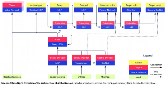
And you can go to “detailed-architecture.txt” to learn things like

the block labeled “Core" is “an LSTM with 3 hidden layers each of size 384” (why 3? why 384? why an LSTM?)

the one labeled “Entity encoder” is “a transformer with 3 layers of 2-headed self-attention [with 128-dim heads and 1024-dim feedforward]” -- this is what DeepMind means when they talk about AlphaStar using transformers, although it’s only 3 blocks, which is way smaller than all the NLP transformers

All of this is pretty mysterious to me.  It’s conventional wisdom by now that getting your architecture/hyperparamters right helps no matter how much data you have (indeed, it’s one of the things you use the data to do), and that simple but somehow “domain-correct” architectures like the transformer can beat convoluted ones planned out by humans using domain knowledge.

Like, compare this to other recent mind-blowers:

AlphaZero was a stack of 19 identical ResNet conv blocks (with some small specialized connectors at the start and end)

GPT/BERT/GPT-2 were between 12 and 48 identical transformer blocks

Yet AlphaStar is this gigantic complicated circuit diagram with all sorts of specialized blocks, with their various specialized knobs set to different, seemingly arbitrary powers of 2.

Are there information bottlenecks in there?  What might be holding it back?  Could the training have been less fancy if the least good aspect of the architecture (whatever it is) were improved?  What if it were simpler but just bigger (the whole thing is about the size of GPT-2-small)?  More fundamentally, why this, out of all the possible things you could do?

[myprogrammingsolver]

PROGRAMMING HOMEWORK SOLUTION

Empirical analysis of algorithms involves implementing, running and then analyzing the run-time data collected against theoretical predictions. This homework asks you to implement, and theoretically and empirically compute the complexities of algorithms with different orders of complexity to solve the problem of Maximum Sum Contiguous Subvector defined as follows: Maximum Sum Contiguous Subvector…

[evanvanness]

Annotated edition of May 10 Week in Ethereum News

I’ve started thinking of the annotated version as aimed at Eth holders.  There’s a large group of people who hold ETH who want to stay up to date on what is happening, but also have jobs outside of the industry and may not understand all the tech nuances nor have time to spend.  So the annotated edition will try to give you more narrative, more context, some opinion, maybe some 🌶️, as well as pointers to what might you want to read

Fun fact: you can find the #MostClicked and #MuchClicked on Twitter by just searching the hashtags. The usual caveats apply: the things most clicked are the things people hadn’t otherwise seen (not necessarily the most important), and my tweets auto-delete after a month or two, so the data only goes back a couple months.

Before clicking send, I knew for sure which would be the most clicked item this week.  I was right.

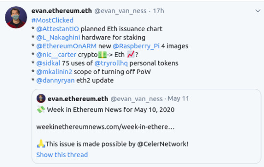
How did I know it would be the most clicked?  Because even among Ethereum enthusiasts it’s an undercommunicated thing how low eth issuance will be.  It is planned to sustainably be so low that it might at some points go negative (and perhaps be negative over long periods of time, which worries me a little!).  Perhaps part of the reason we don’t communicate this that loudly is because we just aren’t there yet.   But unlike Bitcoin which has no path to long-term sustainability, Eth has a logical plan to have very low issuance.  

As I said, I forgot this last week, but if I were clicking a few things this week:

chart of ETH issuance over time

A review of hardware for eth staking

MyCrypto’s history of Eth hard forks to celebrate 10m blocks

I might also check out the stuff about personal tokens, because personal money is an interesting subject to think about, even if you’re skeptical like I am.  The idea of “what is money” can take you down some fun intellectual rabbit holes: 

75 interesting uses of social money by Roll 

Personal tokens were the topic du jour, check out this overview from Dan Finlay

A little light this week on the high-level stuff.  The chart of Eth issuance I already discussed.  The hardware for Eth staking is a worthwhile jumping off point if you’re planning on staking.   And the hard fork history is worth knowing, or if you know it, then it’s a fun trip down memory lane.

Eth1

Step by step guide to running a Hyperledger Besu node on mainnet

Nethermind v1.18.30 query the chain and trace transactions within minutes with Beam sync

A primer on block witnesses

Installation guide to running eth1 nodes (or eth2 testnet) on RaspberryPi4

So this week we have a guide to running the ConseSys’s Besu client (part of Hyperledger) which is a Java client aimed at enterprise, but which can run mainnet.   More Nethermind and Besu nodes are good for client diversity.  So is OpenEthereum (formerly known as Parity), which had a release yesterday.

And if you like running nodes on RaspberryPi4, check that out.

This newsletter is made possible by Celer!

Celer has just released a new state channel mainnet upgrade enabling everyone to easily run a layer-2 state channel node and to utilize the low-cost and real-time transactions enabled by Celer. Game developers with no blockchain knowledge today monetize their games through CelerX gaming SDK that leverages the underlying layer-2 scaling technology with ease. Celer has also released the world’s first skill-based real money game apps where players can join multi-player game tournaments and win cryptocurrency prizes, Follow us on twitter, blog, discord and telegram.

Yay, thanks Celer! 

Eth2

Danny Ryan’s latest quick eth2 update – bug bounties doubled, latest IETF BLS standard

PegaSys’s Teku client is now syncing the Schlesi testnet – which has been much more stable than expected

Latest Prysmatic client update – reducing RAM usage, slashing protection

SigmaPrime’s Beacon fuzzer update, struct-aware, bugs found in Teku and Nimbus

Latest Eth2 networking call, gossipsub v1.1. Ben’s notes

Python notebook to simulate a network partition

Apostille, an Eth1x64 variant

Scoping what is necessary to port eth1 to an eth2 shard and turn off proof of work

Lots of talk of go-live this week. Is it July, q3, or q4?  We need to get audit reports and have multi-client testnets running long-term, though last I checked the Schlesi testnet has been quite stable.  And since publishing the newsletter, now PegaSys’s Teku client is fully validating on Schlesi.

Layer2

Demo of Synthetix on the OVM includes paper trading competition with 50k SNX prizepool. The details of how the Optimistic Virtual Machine enables EVM-in-EVM

Gods Unchained building an NFT exchange with StarkWare

Exit games in state channels

Celer Network’s Orion upgrade makes it easy to run a state channel node

I’m going to set up a Celer node later this week if I have a chance.

Also check out the Synthetix trading competition and help stress test the OVM.

Stuff for developers

Solidity v0.6.7, EIP165 (standard interface detection) support. Also survey results on what devs love and hate about Solidity

Solhint v3 – Solidity linter removes styling rules and recommends prettier Solidity instead

Open Zeppelin ethers.js based console

Etherplex: batch multiple JSON RPC calls into single call

Time-based Solidity tests with Brownie

MythX now has 46 detectors

Quiknode has an online tool to test endpoints

Reading Eth price from Maker’s medianizer v1

Build an app with Sablier’s constant streaming tutorial

Building a bot using MelonJS to automate your Melon fund

StarkWare found a vulnerability in Loopring’s frontend where passwords were being hashed to only 32 bit integers

Even the frontend bugs can get you!  

Ecosystem

A chart of ETH issuance over time. The best I’ve seen

Ethereum Foundation’s q1 grants list

A guide to bulk renewing your ENS names

ethereum.org looking for Vietnamese, Thai, Danish, Norwegian, Hungarian, Finnish, or Ukranian translators

A review of hardware for eth staking

A reminder that many ENS names have now expired and need to be renewed! There’s a 90 day grace period, but do it before you forget.

Enterprise

PegaSys’s Hyperledger Besu suite available on Azure Marketplace and Microsoft’s blockchain devkit now supports Besu

Quorum v2.6 – breaking database schema changes, update to geth v1.9.x

Microsoft continues to make the Ethereum dev experience better, with their VScode extension. 

Governance, DAOs, and standards

How to start a MolochDAO

Options for delegated voting in KyberDAO

EIP2633: Formalized upgradable governance

EIP2628: Header in StatusMessage

I oppose any sort of “formalized upgradeable governance” and I think most do.

Application layer

Use POAP for sybil-resistant voting or to determine Discord channel access

Yield: a revised implementation of Dan Robinson’s yTokens for fixed rate, fixed term loans that give a yield curve

Comparing total value locked in DeFi to unique active addresses

75 interesting uses of social money by Roll

Personal tokens were the topic du jour, check out this overview from Dan Finlay

Strike: perpetual swaps with 20x leverage

POAP as a quasi-KYC layer is pretty interesting to me.  Seems like there are some good uses in Ethereum land.

i’m excited to hear that DeFi will get a yield curve!

Tokens/Business/Regulation

Nic Carter: are stablecoins parasitic or beneficial?

OpenRaise: a continuous offering fundraiser for DAOs

dxDAO’s kickstarter using OpenRaise sold out before public announcement – though the curve is still live, plus a secondary Uniswap market

dxDao’s token is an interesting bit.  Most of the token supply goes to the DXDAO, but it’s an interesting experiment in building completely decentralized apps as a Dao with a community that lately has been burgeoning.  It’s also a bit of a check on rent-seeking because it is a credible threat to excessive fees.

One fun note is that the Uniswap market occurred almost immediately and (almost by definition) trades at a substantial discount to the main market.

General

Aggregatable Subvector Commitments, the future may not involve Merkle trees

This week, Ethereum mined its 10 millionth block.

Here’s MyCrypto’s history of Eth hard forks to celebrate 10m blocks

IPFS releases Testground suite for p2p networking tests

PayPal blocked tokenized real estate startup RealT despite a lack of chargebacks, so they’re switching to Wyre

10,000,000 blocks of Ethereum mainnet!

Capricious censorship in web2 and payments!  I’ve been in PayPal’s shoes managing a card not present merchant account, and so I’m somewhat understanding to them.  You’re trying to keep your fraud rate down in a system that sometimes seems rigged against you.  In RealT’s case, they likely also had large amounts coming through which combined with crypto seems scary to Paypal, even with a low chargeback rate.  

It’s not really anyone’s fault.  The system sucks, and this is why Ethereum matters.

Final note that you can see below in the calendar: RAC’s $TAPE dropped yesterday.  It’s a tradable ERC20 token sold on Uniswap (ie, a pre-set price curve).   Of course the price went from $20 to $1000, as the token is redeemable for a limited edition cassette tape of RAC’s new album Boy.

Housekeeping

Did you get forwarded this newsletter?  Sign up to receive it weekly

Permalink: https://weekinethereumnews.com/week-in-ethereum-news-may-10-2020/

Dates of Note

Upcoming dates of note (new/changes in bold):

May 11 – RAC’s $TAPE

May 12 – MakerDAO Sai shutdown deadline

May 22-31 – Ethereum Madrid public health virtual hackathon

May 29-June 16 – SOSHackathon

June 17 – EthBarcelona R&D workshop

[yahooresearch]

Introducing Similarity Search at Flickr

By Clayton Mellina, Software Development Engineer

At Yahoo, our Computer Vision team works closely with Flickr, one of the world’s largest photo-sharing communities. The billions of photos hosted by Flickr allow us to tackle some of the most interesting real-world problems in image and video understanding. One of those major problems is that of discovery. We understand that the value in our photo corpus is only unlocked when the community can find photos and photographers that inspire them, so we strive to enable the discovery and appreciation of new photos.

To further that effort, today we are introducing similarity search on Flickr. If you hover over a photo on a search result page, you will reveal a “...” button that exposes a menu that gives you the option to search for photos similar to the photo you are currently viewing.

In many ways, photo search is very different from traditional web or text search. First, the goal of web search is usually to satisfy a particular information need, while with photo search the goal is often one of discovery; as such, it should be delightful as well as functional. We have taken this to heart throughout Flickr. For instance, our color search feature, which allows filtering by color scheme, and our style filters, which allow filtering by styles such as “minimalist” or “patterns,” encourage exploration. Second, in traditional web search, the goal is usually to match documents to a set of keywords in the query. That is, the query is in the same modality—text—as the documents being searched. Photo search usually matches across modalities: text to image. Text querying is a necessary feature of a photo search engine, but, as the saying goes, a picture is worth a thousand words. And beyond saving people the effort of so much typing, many visual concepts genuinely defy accurate description. Now, we’re giving our community a way to easily explore those visual concepts with the “...” button, a feature we call the similarity pivot.

The similarity pivot is a significant addition to the Flickr experience because it offers our community an entirely new way to explore and discover the billions of incredible photos and millions of incredible photographers on Flickr. It allows people to look for images of a particular style, it gives people a view into universal behaviors, and even when it “messes up,” it can force people to look at the unexpected commonalities and oddities of our visual world with a fresh perspective.

What is “similarity?”

To understand how an experience like this is powered, we first need to understand what we mean by “similarity.” There are many ways photos can be similar to one another. Consider some examples.

It is apparent that all of these groups of photos illustrate some notion of “similarity,” but each is different. Roughly, they are: similarity of color, similarity of texture, and similarity of semantic category. And there are many others that you might imagine as well.

What notion of similarity is best suited for a site like Flickr? Ideally, we’d like to be able to capture multiple types of similarity, but we decided early on that semantic similarity—similarity based on the semantic content of the photos—was vital to wholly facilitate discovery on Flickr. This requires a deep understanding of image content for which we employ deep neural networks.

We have been using deep neural networks at Flickr for a while for various tasks such as object recognition, NSFW prediction, and even prediction of aesthetic quality. For these tasks, we train a neural network to map the raw pixels of a photo into a set of relevant tags, as illustrated below.

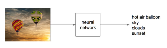
Internally, the neural network accomplishes this mapping incrementally by applying a series of transformations to the image, which can be thought of as a vector of numbers corresponding to the pixel intensities. Each transformation in the series produces another vector, which is in turn the input to the next transformation, until finally we have a vector that we specifically constrain to be a list of probabilities for each class we are trying to recognize in the image. To be able to go from raw pixels to a semantic label like “hot air balloon,” the network discards lots of information about the image, including information about  appearance, such as the color of the balloon, its relative position in the sky, etc. Instead, we can extract an internal vector in the network before the final output.

For common neural network architectures, this vector—which we call a “feature vector”—has many hundreds or thousands of dimensions. We can’t necessarily say with certainty that any one of these dimensions means something in particular as we could at the final network output, whose dimensions correspond to tag probabilities. But these vectors have an important property: when you compute the Euclidean distance between these vectors, images containing similar content will tend to have feature vectors closer together than images containing dissimilar content. You can think of this as a way that the network has learned to organize information present in the image so that it can output the required class prediction. This is exactly what we are looking for: Euclidian distance in this high-dimensional feature space is a measure of semantic similarity. The graphic below illustrates this idea: points in the neighborhood around the query image are semantically similar to the query image, whereas points in neighborhoods further away are not.

This measure of similarity is not perfect and cannot capture all possible notions of similarity—it will be constrained by the particular task the network was trained to perform, i.e., scene recognition. However, it is effective for our purposes, and, importantly, it contains information beyond merely the semantic content of the image, such as appearance, composition, and texture. Most importantly, it gives us a simple algorithm for finding visually similar photos: compute the distance in the feature space of a query image to each index image and return the images with lowest distance. Of course, there is much more work to do to make this idea work for billions of images.

Large-scale approximate nearest neighbor search

With an index as large as Flickr’s, computing distances exhaustively for each query is intractable. Additionally, storing a high-dimensional floating point feature vector for each of billions of images takes a large amount of disk space and poses even more difficulty if these features need to be in memory for fast ranking. To solve these two issues, we adopt a state-of-the-art approximate nearest neighbor algorithm called Locally Optimized Product Quantization (LOPQ).

To understand LOPQ, it is useful to first look at a simple strategy. Rather than ranking all vectors in the index, we can first filter a set of good candidates and only do expensive distance computations on them. For example, we can use an algorithm like k-means to cluster our index vectors, find the cluster to which each vector is assigned, and index the corresponding cluster id for each vector. At query time, we find the cluster that the query vector is assigned to and fetch the items that belong to the same cluster from the index. We can even expand this set if we like by fetching items from the next nearest cluster.

This idea will take us far, but not far enough for a billions-scale index. For example, with 1 billion photos, we need 1 million clusters so that each cluster contains an average of 1000 photos. At query time, we will have to compute the distance from the query to each of these 1 million cluster centroids in order to find the nearest clusters. This is quite a lot. We can do better, however, if we instead split our vectors in half by dimension and cluster each half separately. In this scheme, each vector will be assigned to a pair of cluster ids, one for each half of the vector. If we choose k = 1000 to cluster both halves, we have k2 = 1000 * 1000 = 1e6 possible pairs. In other words, by clustering each half separately and assigning each item a pair of cluster ids, we can get the same granularity of partitioning (1 million clusters total) with only 2*1000 distance computations with half the number of dimensions for a total computational savings of 1000x. Conversely, for the same computational cost, we gain a factor of k more partitions of the data space, providing a much finer-grained index.

This idea of splitting vectors into subvectors and clustering each split separately is called product quantization. When we use this idea to index a dataset it is called the inverted multi-index, and it forms the basis for fast candidate retrieval in our similarity index. Typically the distribution of points over the clusters in a multi-index will be unbalanced as compared to a standard k-means index, but this unbalance is a fair trade for the much higher resolution partitioning that it buys us. In fact, a multi-index will only be balanced across clusters if the two halves of the vectors are perfectly statistically independent. This is not the case in most real world data, but some heuristic preprocessing—like PCA-ing and permuting the dimensions so that the cumulative per-dimension variance is approximately balanced between the halves—helps in many cases. And just like the simple k-means index, there is a fast algorithm for finding a ranked list of clusters to a query if we need to expand the candidate set.

After we have a set of candidates, we must rank them. We could store the full vector in the index and use it to compute the distance for each candidate item, but this would incur a large memory overhead (for example, 256 dimensional vectors of 4 byte floats would require 1Tb for 1 billion photos) as well as a computational overhead. LOPQ solves these issues by performing another product quantization, this time on the residuals of the data. The residual of a point is the difference vector between the point and its closest cluster centroid. Given a residual vector and the cluster indexes along with the corresponding centroids, we have enough information to reproduce the original vector exactly. Instead of storing the residuals, LOPQ product quantizes the residuals, usually with a higher number of splits, and stores only the cluster indexes in the index. For example, if we split the vector into 8 splits and each split is clustered with 256 centroids, we can store the compressed vector with only 8 bytes regardless of the number of dimensions to start (though certainly a higher number of dimensions will result in higher approximation error). With this lossy representation we can produce a reconstruction of a vector from the 8 byte codes: we simply take each quantization code, look up the corresponding centroid, and concatenate these 8 centroids together to produce a reconstruction. Likewise, we can approximate the distance from the query to an index vector by computing the distance between the query and the reconstruction. We can do this computation quickly for many candidate points by computing the squared difference of each split of the query to all of the centroids for that split. After computing this table, we can compute the squared difference for an index point by looking up the precomputed squared difference for each of the 8 indexes and summing them together to get the total squared difference. This caching trick allows us to quickly rank many candidates without resorting to distance computations in the original vector space.

LOPQ adds one final detail: for each cluster in the multi-index, LOPQ fits a local rotation to the residuals of the points that fall in that cluster. This rotation is simply a PCA that aligns the major directions of variation in the data to the axes followed by a permutation to heuristically balance the variance across the splits of the product quantization. Note that this is the exact preprocessing step that is usually performed at the top-level multi-index. It tends to make the approximate distance computations more accurate by mitigating errors introduced by assuming that each split of the vector in the production quantization is statistically independent from other splits. Additionally, since a rotation is fit for each cluster, they serve to fit the local data distribution better.

Below is a diagram from the LOPQ paper that illustrates the core ideas of LOPQ. K-means (a) is very effective at allocating cluster centroids, illustrated as red points, that target the distribution of the data, but it has other drawbacks at scale as discussed earlier. In the 2d example shown, we can imagine product quantizing the space with 2 splits, each with 1 dimension. Product Quantization (b) clusters each dimension independently and cluster centroids are specified by pairs of cluster indexes, one for each split. This is effectively a grid over the space. Since the splits are treated as if they were statistically independent, we will, unfortunately, get many clusters that are “wasted” by not targeting the data distribution. We can improve on this situation by rotating the data such that the main dimensions of variation are axis-aligned. This version, called Optimized Product Quantization (c), does a better job of making sure each centroid is useful. LOPQ (d) extends this idea by first coarsely clustering the data and then doing a separate instance of OPQ for each cluster, allowing highly targeted centroids while still reaping the benefits of product quantization in terms of scalability.

LOPQ is state-of-the-art for quantization methods, and you can find more information about the algorithm, as well as benchmarks, here. Additionally, we provide an open-source implementation in Python and Spark which you can apply to your own datasets. The algorithm produces a set of cluster indexes that can be queried efficiently in an inverted index, as described. We have also explored use cases that use these indexes as a hash for fast deduplication of images and large-scale clustering. These extended use cases are studied here.

Conclusion

We have described our system for large-scale visual similarity search at Flickr. Techniques for producing high-quality vector representations for images with deep learning are constantly improving, enabling new ways to search and explore large multimedia collections. These techniques are being applied in other domains as well to, for example, produce vector representations for text, video, and even molecules. Large-scale approximate nearest neighbor search has importance and potential application in these domains as well as many others. Though these techniques are in their infancy, we hope similarity search provides a useful new way to appreciate the amazing collection of images at Flickr and surface photos of interest that may have previously gone undiscovered. We are excited about the future of this technology at Flickr and beyond.

Acknowledgements

Yannis Kalantidis, Huy Nguyen, Stacey Svetlichnaya, Arel Cordero. Special thanks to the rest of the Computer Vision and Machine Learning team and the Vespa search team who manages Yahoo’s internal search engine.

[ianasennus]

[Udemy] MATLAB Basics for Beginners – Learn from Top Experts

Learn From Top MATLAB Experts In The Field - MATLAB Basics, Data Visualization, Conditions, Loops and much more! What Will I Learn?   Working Knowledge of MATLAB Customize MATLAB to Your Preferences Perform Various Arithmetic Operations with MATLAB Understanding of Vectors Understanding of Matrices Basic Data Visualization Basic Conditional Statements - If/Else Basic Loops Basic Functions Requirements MATLAB already installed on your PC, free license works too No Prior Coding Knowledge is Required You will need ZIP software like WinZip or WinRar, to Unzip/Unrar the Source Code files Desire and Need to Learn MATLAB Description This course will transform you from a MATLAB Novice into a MATLAB Master. The course was developed under the strict oversight of Hristo Zhivomirov who is one of the top 50 MATLAB contributors Worldwide (search for his name in Google).    The course is structured in a way that is suitable for both beginners and those that already have some experience with MATLAB, there is a lot of information for everyone.    Everything in our world today can be viewed as some kind of a matrix, and I’m not talking about the Matrix Trilogy. For example Measuring the temperature of a patient every 2 hours, can be represented with a one dimensional matrix, which is also called a vector   Monochromatic (black and white) image is a two dimensional matrix, the values in each cell in the matrix is representing the gradation of the gray color    Measuring temperature in a room for example, rooms are 3D, so we need x, y, z to describe the position at which we take our measurements, and the value is the temperature, that is a three dimensional matrix    Measure now the change of that temperature over a period of time and the temperature becomes a fourth dimension Now add time in the mix and you get… a fifth dimension! Actually MATLAB has no restrictions on dimensions, you can work with 4, 5, 6 and more dimensions in a single matrix! How to handle The Matrix: It is not necessary to look for the red pill, like Neo had to – what you actually need is MATLAB, which means MATrix LABoratory contrary to popular belief. MATLAB is a programming language of high level and interactive programming environment that lets you easily implement numeric experiments and methods, allowing you to design algorithms, analyze data and visualize that data in a very, very powerful way.  You will learn:    Variables, everything you need to know about variables in matlab, their types or lack of types, converting between different types, naming conventions, the semicolon operator and more    Basic Arithmetic Operations in MATLAB, the most important thing in this section of the course are the Brackets and the Order of operations, many beginners get lost when they encounter complex expressions, and you will become a master of those Right after that we are diving into deep waters starting with Vectors, you will learn how to think in vectors and perform a variety of different operations on and with vectors. Concatenating vectors, extracting or selecting subvectors, and more    Matrices are next on the line, but you wont need any pills, because I have you covered, you will learn everything you need to know about working with Matrices in MATLAB and you will also learn a trick in this section that will help you optimize your code and make it run up to 100 times faster!  Data visualization, because, well, whats the point of working with Data if you cant understand it or share it with other people, visualizing data is key in any area of work    And finally we get to the actual MATLAB Programming by utilizing conditional statements, loops and functions to control the flow of your code, write less code, and make your code modular. Each section contains a source code file at the end so that you can download and review the code that I have written in the lectures! I hope that you will enjoy this course, as much as I did creating it, so lets dive right into it! I welcome you to the course! Who is the target audience? Academics Researchers Engineers Students Anyone who has interest in working with Data source https://ttorial.com/matlab-basics-beginners-learn-top-experts

source https://ttorialcom.tumblr.com/post/177064836798

[ttorialcom]

[Udemy] MATLAB Basics for Beginners – Learn from Top Experts

Learn From Top MATLAB Experts In The Field - MATLAB Basics, Data Visualization, Conditions, Loops and much more! What Will I Learn?   Working Knowledge of MATLAB Customize MATLAB to Your Preferences Perform Various Arithmetic Operations with MATLAB Understanding of Vectors Understanding of Matrices Basic Data Visualization Basic Conditional Statements - If/Else Basic Loops Basic Functions Requirements MATLAB already installed on your PC, free license works too No Prior Coding Knowledge is Required You will need ZIP software like WinZip or WinRar, to Unzip/Unrar the Source Code files Desire and Need to Learn MATLAB Description This course will transform you from a MATLAB Novice into a MATLAB Master. The course was developed under the strict oversight of Hristo Zhivomirov who is one of the top 50 MATLAB contributors Worldwide (search for his name in Google).    The course is structured in a way that is suitable for both beginners and those that already have some experience with MATLAB, there is a lot of information for everyone.    Everything in our world today can be viewed as some kind of a matrix, and I’m not talking about the Matrix Trilogy. For example Measuring the temperature of a patient every 2 hours, can be represented with a one dimensional matrix, which is also called a vector   Monochromatic (black and white) image is a two dimensional matrix, the values in each cell in the matrix is representing the gradation of the gray color    Measuring temperature in a room for example, rooms are 3D, so we need x, y, z to describe the position at which we take our measurements, and the value is the temperature, that is a three dimensional matrix    Measure now the change of that temperature over a period of time and the temperature becomes a fourth dimension Now add time in the mix and you get… a fifth dimension! Actually MATLAB has no restrictions on dimensions, you can work with 4, 5, 6 and more dimensions in a single matrix! How to handle The Matrix: It is not necessary to look for the red pill, like Neo had to – what you actually need is MATLAB, which means MATrix LABoratory contrary to popular belief. MATLAB is a programming language of high level and interactive programming environment that lets you easily implement numeric experiments and methods, allowing you to design algorithms, analyze data and visualize that data in a very, very powerful way.  You will learn:    Variables, everything you need to know about variables in matlab, their types or lack of types, converting between different types, naming conventions, the semicolon operator and more    Basic Arithmetic Operations in MATLAB, the most important thing in this section of the course are the Brackets and the Order of operations, many beginners get lost when they encounter complex expressions, and you will become a master of those Right after that we are diving into deep waters starting with Vectors, you will learn how to think in vectors and perform a variety of different operations on and with vectors. Concatenating vectors, extracting or selecting subvectors, and more    Matrices are next on the line, but you wont need any pills, because I have you covered, you will learn everything you need to know about working with Matrices in MATLAB and you will also learn a trick in this section that will help you optimize your code and make it run up to 100 times faster!  Data visualization, because, well, whats the point of working with Data if you cant understand it or share it with other people, visualizing data is key in any area of work    And finally we get to the actual MATLAB Programming by utilizing conditional statements, loops and functions to control the flow of your code, write less code, and make your code modular. Each section contains a source code file at the end so that you can download and review the code that I have written in the lectures! I hope that you will enjoy this course, as much as I did creating it, so lets dive right into it! I welcome you to the course! Who is the target audience? Academics Researchers Engineers Students Anyone who has interest in working with Data source https://ttorial.com/matlab-basics-beginners-learn-top-experts

[notstatschat]

Statistics on pairs

I'm interested in estimation for complex samples from structured data --- clustered, longitudinal, family, network --- and so I'm interested in intuition for estimating statistics of pairs, triples, etc.   This turns out to be surprisingly hard, so I want easy examples.  One thing I want easy examples for is the relationship between design-weighted $U$-statistics and design-weighted versions of their Hoeffding projections. That is, if you write a statistic as a sum over all pairs of observations, you can usually rewrite it as a sum of a slightly more complicated statistic over single observations, and I want to think about whether the weighting should be done before or after you rewrite the statistic.

The easiest possible $U$-statistic is the variance $$V = \frac{1}{N(N-1)}\sum_{i,j=1}^N (X_i-X_j)^2$$ where Hoeffding projection gives the usual form $$S = \frac{1}{N-1} \sum_{i=1}^N (X_i-\frac{1}{N}\sum_{j=1}^N X_j)^2.$$

These are identical, as everyone who has heard of $U$-statistics has probably been forced to prove.  In fact $$\begin{eqnarray*} S&=& \frac{1}{N-1}\sum_{i=1}^N (X_i - \frac{1}{N}\sum_{j=1}^N X_j)^2\\\\ &=&\frac{1}{N-1}\sum_{i=1}^N \left(\frac{1}{N}\sum_{j=1}^N (X_i-X_j)\right)^2\\\\ &=&\frac{1}{N-1}\sum_{i=1}^N \left(\frac{1}{N}\sum_{j=1}^N (X_i-X_j)\right)^2\\\\ &=&\frac{1}{N(N-1)}\sum_{i,j=1}^N (X_i-X_j)^2 + \frac{1}{N(N-1)}\sum_{(i,j)\neq(k,l)}^N (X_i-X_j)(X_k-X_l)\\\\ \end{eqnarray*}$$ with the second term zero by symmetry, because the $(i,j)$ terms cancel the $(j,i)$ terms and so on.

The idea is that we can estimate $S$ from a sample by putting in sampling weights $w_i$ where $w_i^{-1}$ is the probability of $X_i$ getting sampled, because the sums are only over one index at a time.  We get a weighted mean with another weighted mean nested inside it.   We can reweight $V$ with pairwise sampling weights $w_{ij}$ where $w_{ij}^{-1}$ is the probability that the pair $(i,j)$ are both sampled, because the sum is over pairs.  

Under general sampling, we'd expect the two weighted estimators to be different because one of them depends on joint sampling probabilities and the other doesn't. Unfortunately, the variance is too simple. For straightforward comparisons such as simple random sampling versus cluster sampling all the interesting stuff cancels out and the two estimators are the same. We do not pass `Go' and do not collect 200 intuition points.

The next simplest example is the Wilcoxon--Mann--Whitney test.

Setup

Suppose we have a finite population of pairs $(Z, G)$ , where $Z$ is numeric and $G$ is binary, and for some crazy reason we want to do a rank test for association between $Z$ and $G$.  In fact, we don't {\bf need} to assume we want a rank test, since the test statistics will be reasonable estimators of well-defined population quantities, but to be honest the main motivation is rank tests.  For a test to make any sense at all, we need a model for the population, and we'll start with pairs $(Z,G)$ chosen iid from some probability distribution. Later, we'll add covariates to give a bit more structure.

Write $N$ for the number of observations with $Z=1$ and $M$ for the numher with $Z=0$, and write $X$ and $Y$ respectively for the subvectors of $Z$. Write $\mathbb{F}$ for the empirical cdf of $X$, $\mathbb{G}$ for the empirical cdf of $Y$, and $\mathbb{H}$ for that of $Z$.  

The Mann--Whitney $U$ statistic (suitably scaled) is $$U_{\textrm{pop}} = \frac{1}{NM} \sum_{i=1}^N\sum_{j=1}^M \{X_i>Y_j\}$$ The Wilcoxon rank-sum statistic (also scaled) is $$W_{\textrm{pop}} = \frac{1}{N}\sum_{i=1}^N \mathbb{H}(X_i) -\frac{1}{M}\sum_{J=1}^M \mathbb{H}(Y_j)$$

Clearly, $U_\textrm{pop}$ is an unbiased estimator of $P(X>Y)$ if a single observation is generated with $G=0$ and $G=1$.  We can expand $\mathbb{H}$ in terms of pairs of observations: $$\mathbb{H}(x) = \frac{1}{M+N}\left(\sum_{i=1}^N \{X_i\leq x\} + \sum_{j=1}^M \{Y_j\leq x\}\right)$$ and substitute to get $$\begin{eqnarray*} W_{\textrm{pop}} &= &\frac{1}{N}\sum_{i=1}^N \frac{1}{M+N}\left(\sum_{i'=1}^N \{X_{i'}\leq X_i\} + \sum_{j'=1}^M \{Y_{j'}\leq X_i\}\right) \\\\ & &\qquad - \frac{1}{M}\sum_{j=1}^M \frac{1}{M+N}\left(\sum_{i'=1}^N \{X_{i'}\leq Y_j\} + \sum_{j'=1}^M \{Y_{j'}\leq Y_j\}\right)\\\\ &=& \frac{1}{N(M+N)} \sum_{i=1}^N\sum_{j'=1}^M  \{Y_{j'}\leq X_i\}-\frac{1}{M(M+N)}  \sum_{i'=1}^N \{X_{i'}\leq Y_j\} \\\\ &&\qquad +\frac{1}{N(M+N)}\sum_{i=1}^N\sum_{i'=1}^N \{X_{i'}\leq X_i\} - \frac{1}{M(M+N)}\sum_{j=1}^M\sum_{j'=1}^M \{Y_{j'}\leq Y_j\}\\\\ &=&\frac{M+N}{NM(M+N)}\sum_{i,j} \{X_i>Y_j\} + \frac{NM(M-1)/2-MN(N-1)/2}{NM(M+N)}\\\\ &=&\frac{1}{NM}\sum_{i,j} \{X_i>Y_j\} + \frac{M-N}{2(M+N)} \end{eqnarray*}$$

So,  $$U_\textrm{pop} =  W_\textrm{pop} + \frac{M-N}{2(M+N)}$$ and the two tests are equivalent, as everyone already knows. Again, there's a good chance you have been forced to do this derivation, and you probably took fewer tries to get it right than I did.

Definitions under complex sampling

We take a sample, with known marginal sampling probabilities $p_i$ for the $X$s, $q_j$ for the $Y$s and pairwise sampling probabilities $\pi_{i,j}$.  We write $n$ and $m$ for the number of sampled observations in each group, and relabel so that these are $i=1,\ldots,n$ and $j=1,\ldots,m$.  We write $\hat N$  and $\hat M$ for the Horvitz--Thompson estimates of $N$ and $M$, and $\hat F$ for the estimate of $\mathbb{F}$ (and so on).  That is $$\hat H(z) = \frac{1}{\hat M+\hat N}\left(\sum_{i=1}^n \frac{1}{p_i} \{X_i\leq z\} + \sum_{j=1}^m \frac{1}{q_i} \{Y_j\leq z\}\right)$$

The natural estimator of $W_\textrm{pop}$ is that of Lumley and Scott $$\hat W = \frac{1}{\hat N}\sum_{i=1}^n \frac{1}{p_i}\hat{H}(X_i) -\frac{1}{\hat M}\sum_{J=1}^m \frac{1}{q_i}\hat{H}(Y_j)$$

A natural estimator of $U_\textrm{pop}$ is $$\hat U= \frac{1}{\widehat{NM}} \sum_{i=1}^n\sum_{j=1}^m \frac{1}{\pi_{ij}}\{X_i>Y_j\}$$

Now

 $\hat U$ and $\hat W$ are consistent estimators of the population values

 Therefore, they are also consistent estimators of the superpopulation parameters

However, $\hat U$ depends explicitly on pairwise sampling probabilities and $\hat W$ does not

And there (hopefully) isn't enough linearity to make all the differences go away.

Expansions

We can try to substitute the definition of $\hat H$ into the definition of $\hat W$ and expand as in the population case.  To simplify notation I will assume that the sampling probabilities are designed or calibrated so that $N=\hat N$ and so on (or close enough that it doesn't matter). $$\begin{eqnarray*} \hat W &= &\frac{1}{N}\sum_{i=1}^n \frac{1}{p_i} \frac{1}{M+N}\left(\sum_{i'=1}^n \frac{1}{p_{i'}}\{X_{i'}\leq X_i\} + \sum_{j'=1}^m \frac{1}{q_{j'}} \{Y_{j'}\leq X_i\}\right) \\\\ & &\qquad - \frac{1}{M}\sum_{j=1}^m \frac{1}{q_{j}} \frac{1}{M+N}\left(\sum_{i'=1}^n\frac{1}{p_{i'}} \{X_{i'}\leq Y_j\} + \sum_{j'=1}^m\frac{1}{q_{j'}} \{Y_{j'}\leq Y_j\}\right)\\\\ &=& \frac{1}{N(M+N)} \sum_{i=1}^n\sum_{j'=1}^m\frac{1}{p_iq_{j'}}  \{Y_{j'}\leq X_i\}-\frac{1}{M(M+N)}  \sum_{i'=1}^n \sum_{j=1}^m\frac{1}{p_{i'}q_{j}} \{X_{i'}\leq Y_j\} \\\\ &&\qquad +\frac{1}{N(M+N)}\sum_{i=1}^n\sum_{i'=1}^n \frac{1}{p_{i'}p_{i}} \{X_{i'}\leq X_i\} - \frac{1}{M(M+N)}\sum_{j=1}^m\sum_{j'=1}^m \frac{1}{q_jq_{j'}} \{Y_{j'}\leq Y_j\}\\\\ &=&\frac{1}{MN}\sum_{i,j}\frac{1}{p_iq_j} \{X_i>Y_j\} + \textrm{ugly expression not involving $X$ and $Y$} \end{eqnarray*}$$

(The ugly expression involves the variance of the marginal sampling weights, since $$2\sum_{i,i'} p_i^{-1}p_{i'}^{-1}= (\sum_i p_i^{-1})^2- 2\sum_i p_i^{-2}.$$ It doesn't depend on $X$ and $Y$, and it is the same in, for example, simple random sampling of individuals and simple random sampling of clusters. )

That is, the reweighted $\hat W$ is a version of $\hat U$ using the product of marginal sampling probabilities rather than the joint ones.  They really are different, this time. Using $\hat W$ will give more weight to pairs within the same cluster than to pairs in different clusters.

It’s still not clear which one is preferable, eg,  how will the power of the tests compare in various scenarios? But it’s progress. 

[genetliaco-blog]

View this post on Instagram

A post shared by Subvector (@subvector_band)

3 Agosto! Vi aspettiamo al Penta Metal Fest! 👊🏻 . . . #subvectorband #subvector #concert #penta #metal #rock #rockband #band #newconcert #comingsoon (presso Arcola, Italy)

[genetliaco-blog]

Ecco cosa facevamo noi mentre @meneghinimarco stava incidendo le parti di batteria e Matteo era in conservatorio a studiare.. 😅😅 Che dire, siamo sfatti ma felici! Ci sentiamo domenica per le registrazioni del basso! 😍🎵 #subvectorband #subvector #storm #newalbum #comingsoon #day3 #drumrecording #drums #tamadrums #bullsrecordz (presso BULLS RECORDZ)

[myprogrammingsolver]

PROGRAMMING HOMEWORK SOLUTION

Empirical analysis of algorithms involves implementing, running and then analyzing the run-time data collected against theoretical predictions. This homework asks you to implement, and theoretically and empirically compute the complexities of algorithms with different orders of complexity to solve the problem of Maximum Sum Contiguous Subvector defined as follows:   Maximum Sum Contiguous…

[genetliaco-blog]

Buon natale dai Subvector!! 😂 (...a tra pochissimo con #MidnightPrincess😏) #natale #christmas #christmaspic #cappello #hat #rock #metal #band #subvectorband #auguri

[genetliaco-blog]

Due video dalla serata di venerdì, frammenti di #MidnightPrincess e #DriveMeToTheDawn, i nostri due singoli 🎶🎵 @meneghinimarco on the drums @danielelasorella and Gianluca on guitars Matteo on bass @z123b994 on vocals #rock #metal #rockband #metalband #subvector #subvectorband #contest #concert #massa #ms #theremin #club #italy #tuscany #marco #matteo #gianlu #power #zofia #instafollow #instagram #instalike#instagood #instacool #video #coolvideo #videos #instavideo (presso Theremin Club)

[genetliaco-blog]

Grazie a tutti per la bellissima serata! 🤘🏻 Noi ci mettiamo a lavorare all’album... alla prossima 💪🏻 . . . #subvectorband #subvector #concert #sarzana #music #musica #rock #metal #prog #drum #bass #vocals #guitars #sarzanastock (presso Sarzana)