cgknowhow

[cgknowhow]

GSoC ‘19 Final Report

GSoC is coming to an end. I’m glad to say that I’ve met all the goals as planned in the beginning. You can find out about it in my previous blog posts.

This post is going to be a very brief report of all the things implemented, goals accomplished, some stuff that’s left to do and future plans.

My project was to implement a Data Visualization library in Swift (similar to matplotlib). Before this project, no plotting framework had been written in Swift that could work on Linux, macOS, iOS, or the the other platforms Swift can target. A truly cross-platform Swift plotting framework was needed to fill a gap in the Swift data science ecosystem.

GitHub link to project: https://github.com/KarthikRIyer/swiftplot

What work was done?

The following features were implemented:

1. LineChart #4

2. Plotting functions in LineChart #11

3. SVG Renderer and AGG Renderer as backends. #3

4. Secondary axis in LineChart. #16

5. Bar Chart (both vertical and horizontal, with hatching). #21 #23

6. Scatter Plot (with various scatter patterns). #25

7. Histogram #30

8. Improved aesthetics and text rendering using FreeType. #33

9. A set of examples, to make sure addition of code doesn’t break the existing code. (initiated in #7 with many updates in subsequent PRs).

10. A pure Swift library to generate Jupyter display messages. It is used to display base64 images in a Jupyter notebook. #67

What’s left to do?

Although I’ve completed all the goals as planned, I have started work on a CoreGraphics rendering backend for the iOS and macOS platforms. The PR is currently under review, and little work is left before it is ready to be merged. #35

Also the updated documentation is yet to be merged. This PR has also been submitted for review. #36

Also, the latest work doesn’t work wih Jupyter Notebooks becuase it isn’t able to find the FreeType install on the system when in Jupyter. I haven’t been able to find a fix for this yet.

Future Work

These are some things I plan to work on, post GSoC:

1. Implement an OpenGL Rendering backend.

2. Work on adding support for real-time plotting. For example updating the plot while a machine learning model is training.

3. Implement more complex plot types, such as Contours and Fields.

Highlights and Challenges

A flexible architecture: This approach was slightly new to me. I had to implement an architecture that kept the rendering of primitives as far away from the plotting logic as possible. This provided the necessary flexibility to add more rendering backends when required.

Implementing a pure Swift display library for swift-jupyter: It took me some time to understand how Jupyter worked. I hadn’t ever used Jupyter notebook before, let alone write a library for it. Once I understood how Jupyter worked it was relatively easy to get it to work. But I still faced a few hurdles which were a little tricky to debug. Like, when I was sending a serialized c-string to the Jupyter kernel, it had a next line delimiter at the end. This caused problems with the Jupyter kernel. I required help from my mentors to solve this issue. I also got to explore SHA256 hashing while working on this. It was necessary for message signing. I used IBM’s BlueCryptor library for SHA256.

Allowing more input data types: Deciding which method to use to allow more input data types was time consuming. In the end we settled on generics. Implementing this also took some time, and it was a bit tricky to get the FloatConvertible protocol to work. FloatConvertible was a Swift protocol I wrote which took Numeric input which could be converted into Float. This isn’t perfect yet. It still has some trouble working with the Int Data type.

Working with FreeType: Working with FreeType was a little tricky. I needed a method to draw custom fonts to improve the aesthetics of the plot. Although AGG provides methods that uses FreeType to draw text, I needed a way to use FreeType with Swift Package Manager. One way was to include FreeType with SwiftPlot, but I couldn’t get it to build with Swift Package Manager. FreeType had it’s own build configuration and also had some Python files. The other option was to make Swift Package Manager find the FreeType install on the system, which came with the necessary headers and the compiled binaries. After a lot of legwork I found a way to do that. The next hurdle here was to test it on the macOS platform. I didn’t have a Mac and when I got access to one I wasn’t able to install FreeType on it. After some more legwork I was able to build FreeType on my own and install it from there. This section is also not perfect yet. It isn’t able to find the FreeType install on the system when in a Jupyter Notebook.

Conclusion

I got to learn a lot of things during the summers. I learnt a new language (Swift) and its conventions, approach to building flexible frameworks, how Jupyter works, and many more things. In other words I’ve had a great and productive summer, working under the guidance of the best mentors possible. Brad and Marc (my mentors) were very motivating and their solutions to my problems always worked! 

It was a great feeling to see my project take shape from scratch and even greater to see the community showing interest in it right from the start. I will definitely keep working on this project post GSoC and would like to see a community growing around it, and people contributing to it.

I hope that this project comes to the next GSoC too so that it keeps on maturing and its reach increases more. I would be more than willing to help people get started.

I’ll keep posting updates whenever there are any developments. So stay tuned!!

[cgknowhow]

GSoC Coding Phase - Part 4

Hey everyone!

It’s been a long time since I last posted. Since then I’ve passed the second evaluation, and am pretty close to the end of this years’s GSoC. The final evaluation period starts tomorrow.

This post will be a very brief account of the developments since the last time, and the future plans.

The first topic to address is how we plan to handle data other than Float. After some discussion it was decided that using Generics would be a good option. I wrote a FloatConvertible protocol, and wrote Float and Double extensions conforming to it. The protocol is as shown below:

public protocol FloatConvertible : Comparable{   init<T: FloatConvertible>(_ x: T)   init(_ other: Float)   init(_ other: Double)   init(_ other: Int)

  func toFloat() -> Float   func toDouble() -> Double   func toInt() -> Int   static func +(lhs: Self, rhs: Self) -> Self   static func -(lhs: Self, rhs: Self) -> Self   static func *(lhs: Self, rhs: Self) -> Self   static func /(lhs: Self, rhs: Self) -> Self }

extension Float: FloatConvertible {   public init<T: FloatConvertible>(_ x: T) {self = x.toFloat()}   public func toFloat() -> Float {return Float(self)}   public func toDouble() -> Double {return Double(self)}   public func toInt() -> Int {return Int(self)} }

extension Double: FloatConvertible {  public init<T: FloatConvertible>(_ x: T) {self = x.toDouble()}  public func toFloat() -> Float {return Float(self)}  public func toDouble() -> Double {return Double(self)}  public func toInt() -> Int {return Int(self)} }

Now, each plot class would have generics accepting values conforming to the FloatConvertible protocol. I’m using Floats for calculations at most places. As the input data conforms to FloatConvertible we can convert each value to a Float before any operation. This method also avoids type erasure. Most of you might notice that there’s no extension for the Int data type. That’s because I’m facing some issues with it. Whenever I use Integers I get a fatal error while execution, the reason to which I haven’t been able to figure out yet. So, currently we can use Float and Double.

The next issue I came across was when I was testing plotting different values. I had forgotten to consider a case when the range of values was less than 1, i.e. the plot markers had to have decimal values. So what I did was if the range was between 1 and 2, I plotted each marker with an increment of half times the inverse of the range. And when the range was less than 1, each increment was one-tenth of the range. I also rounded the values to two significant digits. This worked well for most cases.

Brad pointed out that the current plots weren’t as aesthetically pleasing as those generated by currently existing frameworks. The following needed to be changed:

1. Font

2. Line Size

3. Spacing of numbers from axis hatching

4. Enable a grid

Changing the line size, spacing and enabling a grid were simple tasks and didn’t take a lot of time. The tricky part was using a custom font. Let’s take a look at the approach used with both AGG and SVG Renderers.

AGG provides a way to draw text using custom fonts using the FreeType library. Either we need to include FreeType with SwiftPlot or we need a way so that Swift Package Manager can use a version of FreeType installed on the device. I initially wanted to include FreeType with SwiftPlot, but FreeType has its own build system and it also had a few Python files in its source. So I ruled that out. In order to use the install on the device I needed a module that lets SPM know which library to look for. I found this C module on github which with a few changes I got working. Then I changed the old text functions to use the FreeType functions provided by AGG. The default font I used was Roboto-Regular. I had two reasons for choosing this font. One, it was very clean and professional looking. Second, this font was available in the Google Fonts API(This came in useful for SVG).

I couldn’t find any simple way to use custom fonts in SVG that worked everywhere. The only method I found was to use CSS, which worked only in a browser. Brad said that people would use SVG primarily in a browser so supporting that could be a good beginning. The next problem was how to set a default font in SVG? We couldn’t include the font in the SVG file, and including the ttf file along with the SVG file would be very inconvenient. Here the Google Fonts API came in useful. We just need to specify the font family and it would fetch the font whenever the image was loaded into the browser.

This almost concludes my work on aesthetics. The only problem left is to get FreeType to work with Jupyter. Currently, It isn’t able to find the FreeType installed on the system.

Histogram with updated font and grid

Apart from this my main objectives are complete. In the leftover time I have started work on a CoreGraphics Renderer for macOS. This would be a great addition to the library and increase its audience.

That’s all for this post. I’ll post an update when I have CoreGraphics working. Stay tuned!

[cgknowhow]

GSoC Coding Phase - Part 3

The next thing to do was to get Jupyter notebooks to display the plots using pure Swift. Currently this was being done using the EnableIPythonDisplay.swift library bundled with swift-jupyter. The image was being passed to a display function after encoding it to the base64 format. The display function then used IPython’s display function along with the image format(i.e. PNG) to generate a display message, which was then sent to the Jupyter Kernel. And voila! The image was displayed!

For those who don’t know what a Jupyter Notebook is, quoting the Jupyter Notebook website:

The Jupyter Notebook is an open-source web application that allows you to create and share documents that contain live code, equations, visualizations and narrative text.

The way Jupyter displays thing is using messages. A message contains all the data that Jupyter requires to display anything.

The general format of a Jupyter message(as mentioned here) is :

{  # The message header contains a pair of unique identifiers for the  # originating session and the actual message id, in addition to the  # username for the process that generated the message.  This is useful in  # collaborative settings where multiple users may be interacting with the  # same kernel simultaneously, so that frontends can label the various  # messages in a meaningful way.  'header' : {                'msg_id' : str, # typically UUID, must be unique per message                'username' : str,                'session' : str, # typically UUID, should be unique per session                # ISO 8601 timestamp for when the message is created                'date': str,                # All recognized message type strings are listed below.                'msg_type' : str,                # the message protocol version                'version' : '5.0',     },  # In a chain of messages, the header from the parent is copied so that  # clients can track where messages come from.  'parent_header' : dict,  # Any metadata associated with the message.  'metadata' : dict,  # The actual content of the message must be a dict, whose structure  # depends on the message type.  'content' : dict,  # optional: buffers is a list of binary data buffers for implementations  # that support binary extensions to the protocol.  'buffers': list, }

To display images/graphics the message type(msg_type tag in the header) is display_data. 

So what I had to do was, generate such display messages using Swift and send them over to the Jupyter Kernel.

Initially I found it pretty difficult to understand how messaging worked in Jupyter, so I had next to no idea about what I had to do. I decided to give it a few days and i finally started to understand what it all was. I made a naive implementation of the message generating code but only to fail. I got some error which seemed like gibberish to me. Even Googling didn’t help me here. Then Marc came to rescue. In swift-jupyter we send the message to the kernel in a serialized form(a utf8 CString). Marc found that while converting to this form, an extra null terminator was added to it, which created an error with Jupyter. Also in my implementation the message wasn’t an optional. So if a message was empty, it was still getting sent and this caused some errors. So, Marc removed the null terminators and made the message an optional. 

But just sending messages wasn’t enough. Jupyter also needed message signing. A unique signature was generated for each message which was verified by Jupyter and if successful, only then we could see the result appear in the notebook. All this time we wore working by disabling message signing in Jupyter like this:

jupyter notebook --Session.key='b""'

The signature is the HMAC hex digest of the concatenation of:

A shared key (typically the key field of a connection file)

The serialized header

The serialized parent header

The serialized metadata

The serialized content

The hashing function to be used was sha256.

The problem that I faced here was, how do I get the HMAC hex digest? Implementing it on my own was out of question, because there was no way to guarantee its security. There are no cryptographic functions in Swift available on Linux. On Mac we could use CommonCrypto. It is an Obj-C library that one could import using bridging headers between Obj-C and Swift. The obstacle here was that using CommmonCrypto wouldn’t make it cross-platform, and also I had no idea of how to use bridging headers with swift-jupyter. 

Brad suggested that we could use IBM’s BlueCryptor library. This was a cross-platform Swift cryptography library. On the Mac platform it used the CommonCrypto module and on Linux it used the libssl-dev package.

So to use the pure swift library the user had to install BlueCryptor before, or disable message signing.

Using BlueCryptor was pretty straightforward. The exact way to get an HMAC hex digest was given in the documentation. I had a few hiccups doing this initially, because I did not know that the key and data for hashing were to be provided as hex strings. I was using simple strings before and therefore wasn’t getting any results. Also the Swift toolchain I was using had some problems due to which it couldn’t compile BlueCryptor. The only Swift toolchains compatible with swift-jupyter were the S4TF nightly builds, which for some reason didn’t have python3.6 support on that specific day, which was a must for swift-jupyter. So I had to build it myself. This took a lot more time than I expected. 

After all these hassles, finally I got it working. Yipee!!

You can find the implementation here: EnableJupyterDisplay.swift

Then I submitted a PR, which was reviewed many times. The comments were mostly about code formatting and style. I still hadn’t gotten used to the Swift style. I did what was asked and the PR was merged. There is still work to be done on this, like supporting more file formats, maybe include audio playback, etc. But all of that can come later. Right now the focus is just on making the data visualization library.

When I had taken a break from thinking about messaging in Jupyter I got to wotk on fixing the plot dimensions issue with the AGG Renderer.

How the AGG Renderer works is that, on initializing an instance of the renderer creates a buffer that holds all the pixels of the image. One could easily say that to have a custom size, one could pass in the image dimensions in the initializer/constructor of the respective class and allocate a buffer of the required size. But on doing this I got a segmentation fault. On investigating the issue using gdb, I found that the error had to do something with the row_accessor not being able to access a pixel. Essentially we were trying to access a wrong memory location somewhere. But even after going through the code many a times I couldn’t figure out where i was going wrong. The previous implementation had the buffer declared globally. It worked that way, but not when the buffer was part of the class.

I decided to dig a bit deeper and tried to find out answers online. There seemed to be no such answers anywhere but, I found an AGG mailing list, that had been inactive for more than two years. I did not have high hopes, but there was no harm in giving it a try. I’ll add the link to the mailing list at the end if anyone would need it in the future.

class Plot{  public:    agg::rasterizer_scanline_aa<> m_ras;    agg::scanline_p8              m_sl_p8;    agg::line_cap_e roundCap = agg::round_cap;    renderer_aa ren_aa;    int pngBufferSize = 0;    unsigned char* buffer;    agg::int8u*           m_pattern;    agg::rendering_buffer m_pattern_rbuf;    renderer_base_pre rb_pre;    Plot(float width, float height, float subW, float subH){      frame_width = width;      frame_height = height;      sub_width = subW;      sub_height = subH;      buffer = new unsigned char[frame_width*frame_height*3];      agg::rendering_buffer rbuf = agg::rendering_buffer(buffer, frame_width, frame_height, -frame_width*3);      pixfmt pixf = pixfmt(rbuf);      renderer_base rb = renderer_base(pixf);      ren_aa = renderer_aa(rb);      pixfmt_pre pixf_pre(rbuf);      rb_pre = renderer_base_pre(pixf_pre);    }

This was the part of the code I was using to initialize the renderer. I sent this snippet to the mailing list. Fortunately someone called Stephan Abmus responded to my mail and pointed out that all the objects required for rendering needed to stay in memory while rendering. I won’t bore you with excessive details but here is a brief summary. I was declaring the pixf and rendering buffer in the constructor and as soon as it went out of scope those declarations went out of memory too and thus we got an error. I am still not sure why making the buffer global worked. Even declaring the buffer and pixf outside the constructor didn’t help. Actually pixf is a typedef for pix_fmt, which holds the format of the pixel to be used in the image, for example RGBA. In fact I couldn’t declare pixf outside the constructor because it didn’t have a default constructor. I had to pass in the rendering buffer while declarinf the pixf object. This meant I couldn’t declare the rendering_buffer outside of the constructor. The only option left was to declare the rendering buffer object and the pixf object inside every function that renderer something onto the image. This method worked!I had finally fixed the bug I was racking my brains on from the first day!

The next task to accomplish was to provide a better way to give data input to the plots, than the Point type. I was still trying to think of a way to do that. I had tried out generics but at the time it didn’t seem like a viable method. This topic is still under development and once something is finalized I’ll write about it.

The goals for my first milestone were done. 

On June 28, the results of the 1st evaluation were declared. I had finally passed the first evaluation. But I did know beforehand that I’d be passing the evaluation as I had already spoken about it with Brad and Marc. Both of them had given me positive feedback regarding it.

Nonetheless, I’ll describe very briefly what the evaluation was. Both the stuent and the mentors were to fill out an evaluation form. The mentor had to give an evaluation of how well the student had performed, and if he/she should pass or not, and the student had to answer a few questions about their GSoC experience and how well they were able to communicate with the mentors.

Phase 1 went pretty smoothly. There were a few ups and downs, but I’ve the got possibly the best mentors ever who guided me through the whole process. I got to know about Swift, it’s coding format and style. I learnt a lot about building frameworks through my mentors’ answers to  my questions. I observes=d how they think about the features to implement and what kind of implementation would be best for both the developer and the end user of the product.

This was the feedback I received from my mentors. It was a really great motivator for me and I want to give my best now more than ever. 

I hope the rest of the summers stays on to be the great experience I’ve had till now.

I’ve worked on implementing Histogram since then, and I also seem to have made some progress on the Data Input front. I’ll talk about any further developments in the next post.

See you next time! 

[cgknowhow]

GSoC Coding Phase - Part 2

Last time we left off at where I’d implemented some code to display plots in a Jupyter notebook. The next task was to get an independent y-axis working in the Line Graph. I looked at other plotting frameworks’ implementation of this feature. What matplotlib did was that it had different kinds of plots added to an axes, ad the axes was then plotted. To get independent axes, it was twinned with one of the axes. For example if you have a primary axis and twin a secondary axis with it, they will be plotted opposite to each other. ggplot required you to explicity set the scale for the secondary axis relative to the primary axis. After some thinking I decide that having a primary and secondary axis with series of data being added to either one of them would be a good options. The scaling would be done automatically of course. But how would you differentiate between a plot on either axis? A simple solution for now could be to make the secondary plot lines dashed, so that’s what I went with. Remember I had told you that setting up the tests in the beginning helped me with a bug? While implementing multiple y axes, I gave negative input points for the first time and noticed that I hadn’t though of this while implementing the logic. I could easily check the difference in old and new plots by using git. If the newly rendered image was different it would show up as updated in git. I had lifted the logic directly from Graph-Kit the android library I’d made and it seems I’d made that mistake there too. So I spent some time rectifying that.

The next task was to implement Bar Graph. This seemed like an easy enough task as I distinctly remembered it to be less work even when implementing it in Graph-Kit. Bu this time I didn’t repeat the same mistake as I did with Line graph. Although I did initially lift the logic again I immediately checked for loopholes such as negative coordinates. I had to rewrite some of the code to get that done. Additional features planned for Bar Graph were plot hatching and stacked plots. Hatching is the patterns you fill inside the bars, something like shading the bars. For implementing hatching there were two options. One was to use primitives to generate the patterns. As this would be implemented using primitives everything could be done using Swift. This would make all the renderers support hatching. The other option was to have an enum/list of possible hatching patterns and pass a unique value for each case to the renderer and all the pattern generation will be handled independently by the renderer. This meant that each renderer implementation would need to have some logic to generate the patterns, and maybe some renderers would not have out of the box support for this. The former had some disadvantages. If we generated all the pattersn in Swift using primitives we’d have to handle the edge cases i.e when half of a pattern was inside the rectangle and half of it outside, we’d have to clip it. Then there would also be the logic for drawing the pattern in the bound area of the rectangle. Basically we’d have to reinvent the wheel. Even if this was done, in the case of SVG, a lot of statements to render primitives would be added to the file. This would take a lot of time to parse and therefore delay the final image generation. Both the renderers I was using had the pattern generation feature built right into them. They would easily handle all edge cases and filling the pattern in the required area. So I went with the second option. I just had to implement some logic to generate the shapes to be used in the hatching pattern. The patterns I implemented were forward slash backward slash, hollow circle and grid to name a few. Then I went on to implement stacked bars. This could be used when multiple series of data were to be plotted on the came graph. The next series of data was placed over or below the previous series’ bar depending on whether the data point was positive or negative. There were no specific challenges to this other than the usual debugging one does to get any feature working. The last part left in Bar Graph was to allow horizontal bars too. I just had to switch the x and y values if the graph was to be plotted horizontally.

I went on to implement Scatter Plot. This wasn’t a very difficult task as the logic was pretty much the same as that of Line Graph, the difference being that the line weren’t to be joined by lines and instead be replaced with shapes. I added functions to the renderers to draw triangles and polygons. Generating the points to draw shapes like triangle, hexagon, stars was simple trigonometry and rotation of points. I also added a helper function to rotate points about a center. This wrapped up Scatter Plot.

While implementing Bar Graph, the plot had to accept String input also. So I had to add String variables to the Point type. This raised a question. Was the current way of using Point to accept data the correct way? We had to think of other ways to support other data types such as Double, Int, etc. Is generics the right way to proceed? This is a topic that’s currently under discussion. 

Meanwhile I started work on a python free implementation to display plots in Jupyter Notebooks. I also simultaneously fixed the plot dimensions issue with the AGG Renderer. I’ll discuss this next time, so stay tuned!

[cgknowhow]

GSoC Coding Phase - Part 1

Hello everyone!

A lot has happened since the GSoC results were declared! I’ve got quite a few things implemented in my project, I’ll be breaking the discussion of the first part of the coding phase into two or three parts. So lets get into it without further ado.

According to my proposal here, I had one week of community bonding, during which I had to make sure that I had everything I needed to begin with the project, and discuss with the mentors what i should be doing ahead of time. I received a mail from my mentors, Brad and Marc welcoming me to the program. After some discussion it was decided that I should modify my milestones a little bit. Swift for TensorFlow is being used in the Fast.ai course. And there’s a lot of interest in displaying plots in Jupyter notebooks, which is being driven by this. This was to be moved to the first milestone. I have never worked with Jupyter notebooks before let alone editing code that communicated with a Jupyter Kernel. Marc guided me through this. It was decided that for an initial implementation I could use the Swift-Python interoperability to display base64 images in a relatively straightforward manner. Once I implemented some of the planned plots I could work on a pure Swift implementation.

One of the most important parts of building a framework is that it functions as expected. There will definitely be many revisions and changes to the code later on. This warranted a need for the presence of some tests included in the project repository. This would help in making sure that new changes did not break the previously working plots. (I am really glad that we decided to include this in the first milestone itself. It helped me find a really important bug! We’ll come to it in later on)

I have been a little vague in my proposal about implementation of Sub Plots. For those who don’t know what Sub Plots are, they are multiple graphs included in a single display/image. They can be of any type(Line Graph, Bar Graph, etc.). It was necessary to include Sub Plots in the first milestone itself because each Plot would have to be coded in a way that it could be part of a Sub Plot. Implementing all the plots independently and later adding Sub Plot support would be a lot of extra work!

So this is what was decided. In the first milestone I would do the following:

Make a simple Line Chart implementation with Sub Plot support.

Setup tests that saves images.

Get a base64 encoded PNG and use it in Jupyter notebook. Later work on python free implementation.

Complete line chart implementation in the leftover time.

The rest of the stuff for the first milestone according to my proposal were to be moved to the second milestone.

It didn’t take long for me to complete the simple line chart. I used most of the code from the prototype I had made with a few changes.

Let’s look briefly at the LineGraph implementation. All the further discussion will be applicable to Linux (I am using Ubuntu 18.04 LTS) unless otherwise specified.

The first step was to set up the Swift Package. For absolute beginners, this is how you initialise a Swift Package using the Swift Package manager:

Execute this command in the terminal.

swift package init --type library

This will initialise a package that is primarily meant to be a library. If you want a package with an executable as the build product, you can change the type flag to executable.

Before implementing the plots I had to set up the renderers because they were the entities that would handle all the image generation. The plan was to have almost no plotting logic in the Renderers. They would just allow you to draw primitives such as Lines, Rectangles, Text, etc.

One of the Renderers part of the project is the Anti-Grain Geometry C++ library, developed by the late Maxim Shemanarev. I wrote some code to render simple primitives necessary for a Line Graph. Although Swift Package Manager can compile C++ code, C++ functions aren’t directly accessible from Swift code. So I had to write a bridging C-headers. You can call the C-functions from Swift directly which in turn call the C++ functions. You can find the implementation here.

One other aim of implementing different rendering backends was to facilitate adding more backends in the future. This required all the Renderers to have some main stuff in common. So I made a Renderer protocol that included the main functions that every Renderer must have. Each Renderer will have to conform to that protocol. 

The AGGRenderer worked fine apart from one thing. The plot dimensions and and therefore the buffer size were hard coded. This meant that the user couldn’t change the size of the image rendered. This was obviously a big handicap to the end user. But for the moment I decided to focus on implementing the plot and getting the basic structure up and running. I could deal with it later on.

The other Renderer I planned to implement was a simple SVGRenderer written in Swift. The implementation is pretty simple and straightforward just like the SVG format. It has a String variable that will describe the image. Whenever you need to draw a primitive you pass the data to the SVGRenderer and it concatenates the relevant tag to the String. In the end the Renderer saves the String into a .svg file. 

We’re talking about passing the plotting data to the Renderer, but how does that happen? I have defined a Point type which is a struct. It contains two Floats, x and y.  You can pass the plotting data to the Renderer in the form of Point variable, or Point arrays. But the end user need not worry about this. All this will be handled by the Plots. Which brings us to the LineGraph implementation.

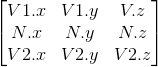
What I noticed first was that each plot would have to have the support of being a SubPlot. Therefore the renderer would need each image and plot to have separate dimensions in case of a SubPlot.  Lets take an example of two SubPlots stacked horizontally. An easy way to go about it would be to do all the plot calculations of each plot in its own independent co-ordinate system and the shift the origin of each plot as required while drawing it.So what I did was create a Plot protocol with a PlotDimensions type that held the image size and the dimesions of the current plot being rendered, and two offset variables, xOffset and yOffset respectively. In this case the xOffset of the second SubPlot will be a positive number and the yOffset will be zero for both of them. The plot dimensions will be equal divisions of the net image space available to all the Sub Plots. The Renderer will just shift the origin of each SubPlot by (xOffset, yOffset). This did the job. 

The Plot protocol has just one more method called drawGraph(). This was because each Plot had to have the functionality to just draw the plot in memory irrespective of what mode of output(like saving images in case of AGG, or displaying an image in a window in case an OpenGL implementation was written) the used Renderer would have. Also this facilitated drawing each SubPlot separately to the image before generating the final output. 

Then I took the plotting logic from my prototype and the basic Line Graph was done. 

The next step was to set up the tests. I created an examples directory with individual executable modules, each demonstrating a single feature. In this directory I made a Reference directory with two separate directories for AGG and SVG renders. So that anyone could run all the tests easily in one go, I made a simple bash script with the commands to run each example like so:

swift run <Executable Example Module Name>

Then came the time to let the users show the plots in a Jupyter Notebook. Initially the way I did this was, save the image as usual using the AGGRenderer, re read it from the disk encode it to base64 in C++ code, and send back the String to Swift code. But there was a better way that my mentors suggested. The library that I was using to encode PNGs, lodepng, allowed you to encode the image in memory and not save it to the disk. I could return a pointer to a buffer with the encoded bytes, to the Swift code and use some functions under Foundation to do the base64 encoding in Swift itself. This could come in handy sometime later if another Renderer could generate images that coudl be encoded to base64. I did the encoding using a function like this:

public func encodeBase64PNG(pngBufferPointer: UnsafePointer<UInt8>, bufferSize: Int) -> String {    let pngBuffer : NSData = NSData(bytes: pngBufferPointer, length: bufferSize)    return pngBuffer.base64EncodedString(options: .lineLength64Characters) }

To display the image in Jupyter I added these lines to the EnableIPythonDisplay.swift file in the swift-jupyter repository:

func display(base64EncodedPNG: String) {  let displayImage = Python.import("IPython.display")  let codecs = Python.import("codecs")  let imageData = codecs.decode(Python.bytes(base64EncodedPNG, encoding: "utf8"), encoding: "base64")  displayImage.Image(data: imageData, format: "png").display() }

To display the plot the only thing the user has to do is to include this file in their jupyter notebook, get the base64 image from the plot object and pass it to the display function.

This completed all the main stuff I had planned for my first milestone well before the deadline. By this time the official coding period hadn’t started yet. The first deadline was June 24 and I had almost a month left. I could cover a lot more stuff in my first milestone itself, so I decided to complete the Line Plot and keep at least the Bar Chart implementation in my first milestone.

You can find all the code here.

This post has already gotten pretty long, so I’ll sign off here. I’ll be discussing the rest of my Line Graph implementation, Bar Chart implementation and how setting up the tests beforehand helped me avoid a bug, all in my next post.

Stay tuned!

PS: Don’t forget to subscribe to the Swift for TensorFlow newsletter to stay up to date with the work being done and the happenings of the S4TF community!

Here’s the link: https://www.s4tfnews.com/

PPS: Also recently a Swift for TensorFlow Special Interest Group has been announced to help steer the framework. Weekly meetings will be held discussion the progress and plan ahead. Anyone interested can sign up to the mailing list here.

[cgknowhow]

GSoC with TensorFlow

Hello everyone!

I’ve been selected as a Google Summer of Code developer under TensorFlow. Yaay! 

It’s been a long time since the results came out, and I’ve finally got around to writing about it... so my next few posts will be about my GSoC experience with TensorFlow.

Let’s start at the very beginning...a very good place to start...

January 2019

It was that time of year when everyone was gearing up for GSoC. The organisations for 2019 were to be announced on February 27.  There were many who had already started to contribute to open-source organisations that came to GSoC in the past years, to get a head start. This was the most frustrating experience of my life, because I was having a hard time choosing an organization. I had been exploring computer graphics for the past few months and really wanted to do something in that area...But which org to choose...I was also in doubt if the organizations that came last year would come this year or not...

February 2019

Finally on February 27, the list of orgs was out...I had almost given up, but that day I received a message from a senior at college, that TensorFlow had come to GSoC this year and there was a project that would interest me, something related to Data Visualisation. I was a bit confused if I would be able to contribute or not, considering that TensorFlow was an organisation working in Machine Learning. There was no harm in taking a look at the projects, so I did...

The idea my senior was talking about caught my eye. The idea was:

A library for data visualization in Swift

Once data has been cleaned and processed into a standard format, the next step in any data science project is to visualize it. This project aims to provide a Swift library similar to matplotlib. Desired features:

1. Two-dimensional plots: horizontal and vertical bar chart, histogram, scatterplot, line chart 2. Support for images, contours, and fields 3. Support for detailed subplots, axes, and features Desired languages: C, C++, Swift

I immediately decided to apply for this project. I had made a plotting framework for Android before and this seemed to be something similar but way more involved. I’d have to work with Swift, a language I hadn’t worked with before. It included graphics work that I wanted to do and I would be working under the guidance of people from the TensorFlow team! This seemed like a great opportunity to learn something new.

It turned to to be exactly that. I enquired about the project and guidelines on the Swift for TensorFlow mailing list. I got excellent guidance from the project mentors Brad Larson, Marc Rasi and other community members. I did some digging on my end, got a prototype working and shared it with the S4TF community.

March 2019

Then came the time to work on my proposal. The projects aim was to make a Swift library that works cross-platform. Currently available Swift plotting frameworks worked only on Mac and iOS. So the library had to have multiple rendering backends so that the end user may choose one that worked best on their platform. It was important that I implement at least two rendering backends, so that the library would be architectured in a way that made it simple enough to add more backends later on. After several reviews and revisions from the mentors I finalised my proposal and made the submission on March 25.

Then next month went into preparing and appearing for my end semester examinations, but GSoC results were always on my mind.

May 2019

My exams were over and the results were to be declared in 6 days. 

On 7 May I received a mail:

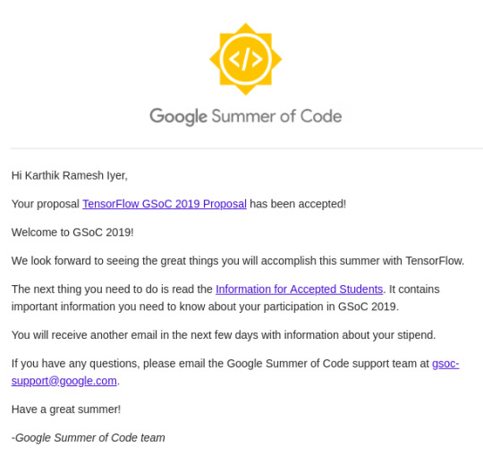
Thus began my GSoC journey with TensorFlow.

Next time I’ll discuss how I got started with my project and share some brief implementation details. Stay tuned!

[cgknowhow]

Here's the result of our work during last Summer. Graph-Kit: An Android Library to plot and edit graphs https://github.com/jsuyash1514/Graph-Kit https://www.instagram.com/p/Bq67SHolUvIbHzeloeF2fYHir_amJ45P6MEQUU0/?utm_source=ig_tumblr_share&igshid=daicc2mk1vo1

[cgknowhow]

Android Vector Drawables

There are two basic ways an image can be represented in: Bitmaps and Vector Drawables. Normal Bitmaps are represented in the form of pixels in a grid. A Vector Drawable  defines the image in the form of geometry, i.e as a set of points in the Cartesian plane, connected through lines and curves, with their associated color information.

In this post we’ll be focusing on static Vector Drawables and some of their advanced features. Animated Vector Drawables will be covered very briefly.

Why Vector Drawables?

Vector Drawables are,

Sharp

All Bitmaps have a specific resolution, which when displayed on a different density display may pixelate or might introduce unwanted artifacts. Vector Drawables look sharp on each display independent of display density, i.e. the same file is resized for different screen densities.

Small

A Bitmap of higher resolution means more pixels. More pixels means larger file size. Vector Drawables do not store pixels therefore they are of the same size independent of display density. This results in smaller APK files and less developer maintenance.

Flexible

Vector Drawables are highly flexible. One can also animate them using multiple XML files.

The support for Vector Drawables was added in API Level 21(Lollipop). Prior to this release if anyone wanted to represent images through Vector Graphics they had to do it manually though Java Code. If Bitmaps were used, developers had to use different images, one for each display resolution. Imagine using animated Bitmaps in such a situation!

There are two classes that help you use Vector Drawables: VectorDrawable and AnimatedVectorDrawable.

There are two basic ways an image can be represented in: Bitmaps and Vector Drawables. Normal Bitmaps are represented in the form of pixels in a grid. A Vector Drawable  defines the image in the form of geometry, i.e as a set of points in the Cartesian plane, connected through lines and curves, with their associated color information.

In this post we’ll be focusing on static Vector Drawables and some of their advanced features. Animated Vector Drawables will be covered very briefly.

The VectorDrawable Class

This class defines a static drawable object. It is defined in a manner similar to the SVG format.

Image Courtesy: developer.android.com

It follows a tree hierarchy consisting of groups and paths. The path contains the actual geometric data to draw the object. The group contains data for transformation of the shape. The path is always a leaf of the tree. The path will be joined in same order in which it appears in the file.

The group text is an internal node of the tree. A path object inherits all the transformation of it’s ancestor groups.

Let’s take a look at a sample Vector Graphic as an SVG file and its corresponding XML Vector Drawable.

SVG

<svg xmlns="http://www.w3.org/2000/svg" width="24" height="24" viewBox="0 0 24 24">

<path fill-opacity=".3" d="M15.67 4H14V2h-4v2H8.33C7.6 4 7 4.6 7 5.33V8h5.47L13 7v1h4V5.33C17 4.6 16.4 4 15.67 4z"/>

<path d="M13 12.5h2L11 20v-5.5H9L12.47 8H7v12.67C7 21.4 7.6 22 8.33 22h7.33c.74 0 1.34-.6 1.34-1.33V8h-4v4.5z"/>

<path d="M0 0h24v24H0z" fill="none"/>

</svg>

XML

<?xml version="1.0" encoding="utf-8"?> <vector xmlns:android="http://schemas.android.com/apk/res/android"    android:width="24dp"    android:height="24dp"    android:viewportWidth="24"    android:viewportHeight="24">    <path        android:fillColor="#000000"        android:fillAlpha=".3"        android:pathData="M15.67 4H14V2h-4v2H8.33C7.6 4 7 4.6 7 5.33V8h5.47L13 7v1h4V5.33C17 4.6 16.4 4 15.67 4z" />    <path        android:fillColor="#000000"        android:pathData="M13 12.5h2L11 20v-5.5H9L12.47 8H7v12.67C7 21.4 7.6 22 8.33 22h7.33c0.74 0 1.34-0.6 1.34-1.33V8h-4v4.5z" />    <path        android:pathData="M0 0h24v24H0z" /> </vector>

This Vector Drawable renders an image of a battery in charging mode.

There’s a lot more you can do with Vector Drawables. For example you can specify the tint for the image. You needn’t worry if the SVG the designer gave has the right shade of grey you need. The same Vector Drawable renders with different colors according to the set theme.

The same image rendered in a light and dark theme.

(Image Courtesy: Android Dev Summit ‘18)

All you need to do to set the tint is add this attribute to the vector:

android:tint="?attr/colorControlNormal"

You can also use theme colors for specific parts of your image. For example in order to use colorPrimary in you image add this attribute to your path:

android:fillColor="?attr/colorPrimary"

The same images rendered with different primary colors.

(Image Courtesy: Android Dev Summit ‘18)

Many a times we need to change the color of icons depending on the state of the button. These changes might be as minor as a different colored stroke. You can accomplish this using different colored images, but when the rendering is the same for most of the part, using ColorStateList inside the Vector Drawable is a much better way. You can avoid a lot of duplication in this manner.

The way to accomplish this is the same as that of a regular ColorStateList. Create a ColorStateList in the color resource directory, and use a reference to it in the fillColor attribute in the path.

If your ColorStateList is csl_image.xml, the add this line:

android:fillColor="@color/csl_image"

Vectors also support gradients. You can have three types of gradients:

Linear

<gradient android:startColor="#1b82bd"android:endColor="#a242b4" android:startX="12" android:endX="12" android:startY="0" android:endY="24" android:type="linear"/>

(Image Courtesy: Android Dev Summit ‘18)

Radial

<gradient android:startColor="#1b82bd"android:endColor="#a242b4" android:centerX="0" android:centerY="12" android:type="radial"/>

Sweep

<gradient android:startColor="#1b82bd"android:endColor="#a242b4" android:centerX="0" android:centerY="12" android:type="sweep"/>\

(Image Courtesy: Android Dev Summit ‘18)

We can also define individual color stops using <item> tag to get more fine grained gradients as show below:

<gradient...> <item android:offset="0.0"          android:color="#1b82bd"/> <item android:offset="0.72"          android:color="#6f5fb8"/> <item android:offset="1.0"          android:color="#a242b4"/> </gradient>

This sets the color at 72% of the gradient direction parameter.

(Image Courtesy: Android Dev Summit ‘18)

Just as we define ColorStateLists in the color resource directory, we can define gradients and then add their reference in our Vector Drawable in the fillColor attribute.

An alternative to this is to define the gradient using inline resource syntax to embed it inside the vector definition itself as shown below.

<vector...>      <path...> <aapt:attr name="android:fillColor">      <gradient        android:type="sweep"        android:centerX="0"        android:centerY="0"        android:startColor="#1b82bd"        android:endColor="#a242b4"

     </aapt:attr>

     </path> </vector>

Here the AAPT(Android Asset Packaging Tool) will extract this to a color resource at build time and insert a reference for it.Gradients are very useful in situations where you need shadows in Vector Drawables. Vector don’t support shadows, but it can be faked using gradients. You can also use it to create customised spinners using a radial gradient.

If the gradient doesn’t fill the entire image, you may choose to so any of the following:

Clamp

This is the default mode. It just continues the color outwards from the last offset point

You may accomplish this by adding the following line in the gradient:

<gradient...  android:tileMode="clamp"/>

(Image Courtesy: Android Dev Summit ‘18)

Repeat

This repeats the gradient until the whole image is filled.

You may accomplish this by adding the following line in the gradient:

<gradient...  android:tileMode="repeat"/>

(Image Courtesy: Android Dev Summit ‘18)

Mirror

This goes back and forth through the gradient.

You may accomplish this by adding the following line in the gradient:

<gradient...  android:tileMode="mirror"/>

(Image Courtesy: Android Dev Summit ‘18)

We can also make gradients that do not go from color to color but have regions of solid color.

This can be accomplished by using the same color between two color stops, as shown below:

<gradient...> <item android:offset="0.0"          android:color="#1b82bd"/> <item android:offset="0.5"          android:color="#1b82bd"/> <item android:offset="0.5"          android:color="#a242b4"/> <item android:offset="1.0"          android:color="#a242b4"/> </gradient>

Vector Drawables are great to reduce the size of the APK file, and reduce the number of images required.They are extremely flexible, but sometimes they come with a significant performance trade-off. Therefore VectorDrawables should be used only when the image is simple up-to a maximum size of 200 x 200 dp, for example icons for Buttons. Shapes should be used instead of Vector Graphics wherever possible.

The AnimatedVectorDrawable Class

This class adds animation to the properties of a VectorDrawable. We can define animated vector drawables in two ways:

Using three XML files

A VectorDrawable file, an AnimatedVectorDrawable file and an animator XML file.

Using a single XML file

You can also merge related XML files using XML Bundle Format.

To support vector drawable and animated vector drawable on devices running platform versions lower than Android 5.0 (API level 21), VectorDrawableCompat  and AnimatedVectorDrawableCompat are available through two support libraries: support-vector-drawable and animated-vector-drawable, respectively.

Support Library 25.4.0 and higher supports the following features:

Path Morphing (PathType evaluator) Used to morph one path into another path.

Path Interpolation Used to define a flexible interpolator (represented as a path) instead of the system-defined interpolators like LinearInterpolator.

Support Library 26.0.0-beta1 and higher supports the following features:

Move along path The geometry object can move around, along an arbitrary path, as part of an animation.

For more information about Animated Vector Drawables you can refer to the links posted at the end of the post.

Performance trade-off for Vector Drawables

Although the XML file used for Vector Drawables is usually smaller than conventional PNG images, it has significant computational overhead at runtime in case the drawn object is complex. When the image is rendered for the first time, a Bitmap cache is created to optimize redrawing performance. Whenever the image needs to be redrawn, the same Bitmap cache is used unless the image size is changed. So, for example you rotate your device, if the size of the rendered image remains the same, it will be rendered using the same cach otherwise the cache will be rebuilt. Therefore in comparison to raster images they take longer to render for the first time.

As the time taken to draw them is longer, Google recommends a maximum size of 200 x 200 dp.

Conclusion

Vector Drawables are great to reduce the size of the APK file, and reduce the number of images required.They are extremely flexible, but sometimes they come with a significant performance trade-off. Therefore VectorDrawables should be used only when the image is simple upto a maximum size of 200 x 200 dp, for example icons for Buttons. Shapes should be used instead of Vector Graphics wherever possible.

Useful Links

Adding multi-density vector graphics in Android Studio

Optimizing the Performance of Vector Drawables

Harnessing the Power of Animated vector Drawables

Vector Drawables Overview

Advanced VectorDrawable Rendering (Android Dev Summit '18)

[cgknowhow]

Path Tracing and Global Illumination

Introduction

Path Tracing is a Monte Carlo method of rendering realistic images of 3-D scenes by simulating light bounces around the scene.

We can speak of illumination in a scene in two ways – Direct and Indirect Illumination. Direct Illumination is due to the light received by objects directly from the light sources. When observe the real world, occluded objects are never completely dark. This is because they receive light reflected off other nearby objects. This is Indirect Illumination.In the Path Tracing algorithm we need to simulate both these effects.

Tracing rays from the light sources in the scene to the camera is very inefficient. A lot of computational power is wasted in tracing rays that won’t ever reach the camera. The solution for this is backward ray-tracing. We shoot rays from the camera into the scene and if the ray finally reaches a light source we can calculate the point’s illumination.

We’ll consider only point light sources and diffuse materials for further discussion, specifically Lambertian materials. The property of Lambertian materials is that they appear equally bright when viewed from any angle. The luminous intensity obeys Lambert’s cosine law. According to this law the radiant intensity or luminous intensity observed, from an ideal diffusely reflecting surface or ideal diffuse radiator is directly proportional to the cosine of the angle θ between the direction of the incident light and the surface normal.

Direct Illumination

Calculating Direct Illumination is pretty straightforward. Consider a single pixel for which we need to calculate illumination. Get the point of intersection of the ray cast into the scene by iterating through the objects in the scene, calculate its distance from the camera. If the distance is lesser then any previous distance calculated for the pixel under consideration, check if the point is shadowed by any other object. The way to do this is to cast a ray from the point towards the light source and check if the ray intersects any other geometry other than the light source. If it is shadowed there’ll be no direct illumination on that point. This gives us an image with completely dark shadows, which is not how the real world looks.

Direct Illumination

Indirect Illumination

The way we’ll use to calculate Indirect Illumination is MonteCarlo Integration.

The above equation is the simplified version of the Rendering equation given by Jim Kajiya. The LHS is what we need to calculate. It the the radince at the given point. In other words it is the colour of that point. L(ωi) is the radiance received at that point from the direction ωi. BRDF is the Bidirectional reflectance distribution function. It includes the colour and properties of the surface. For lambertian surfaces the BRDF is ρ/π, where ρ is the albedo of the surface. Albedo is the ratio of the light reflected to the light received by the surface.  The π in the denominator is the energy conserving coefficient. The light energy leaving the surface after scattering can never be more than what the surface received. Therefore,

where Cd is a constant.

The incoming light is fixed, therefore,

δω is a direction in the unit sphere with centre at the point under consideration. Writing the above equation in polar coordinates:

On integrating we get,

So, if we want to keep the diffuse material colour between 0 and 1 we need to divide it by  π.

To integrate the function at the point under consideration we’ll cast a number of secondary rays from the point into the scene and trace them recursively. Monte Carlo method work when we choose our sample randomly. So the next problem we need to tackle is sample of direction in a unit hemisphere with centre at the point under consideration.

This is a Monte Carlo estimator with probability distribution function pdf(x).

Any PDF must integrate to 1 over the sample space. In our case each sample is equally probable so out PDF will be a constant.

p(ω) is a constant so it comes out to be 1/2π.

We need to generate the samples in polar coordinates and not solid angle ω.

Therfore,

p(θ,ϕ) dθ dϕ = p(ω) dω

p(θ,ϕ) dθ dϕ = p(ω) sinθ dθdϕ.

p(θ,ϕ) = p(ω)sinθ,

p(θ,ϕ) = sinθ/ 2π

In our case, the pdf is seperable, which means that we can say

p(θ) = sinθ

p(ϕ )= 1/ 2π

To sample from the above PDF we need to find the Cumulative probability distribution function and then find its inverse.

Inverting the CDF

y = 1 − cosθ,

θ = cos−1(1−y)

As y is some random number between 0 and 1, 1-y will also be distributed uniformly between 0 an 1. So we can replace 1-y by y.

y=ϕ/ 2π

ϕ=y* 2π

We can then choose x and z to get a unit vector.

Creating a Co-ordinate System

The above method generates random samples in a coordinate system centred at the origin. But, we need samples at a point on one of the objects of the scene. Therefore we need to create another coordinate system at that point, generate samples and then convert the samples back to world coordinates.

Let the normal be at origin.

Consider a plane with the equation Nx *x + Ny∗ y + Nz∗ z = 0.

If we choose a vector with y-coordinate as 0, we get Nx *x + Nz∗ z = 0.

This will be satisfied when Nx * x = −Nz * z.

So, choose one vector as Vector(N.z, 0, -N.x) or Vector(-N.z, 0, N.x). --> V1

To get the third vector(V2) we can calculate the cross product of the Normal with the above vector,

and there we have a coordinate system oriented along the normal at the point under considertion.

If the normal’s y coordinate is greater than he x coordinate it is better to choose the first vector with x coordinate zero, for the sake of numerical robustness. Then, the vector would be Vector(0, -N.z, N.y).

Transform sample to World Co-ordinates

To transform our sample to world coordinates we multiple it by a matrix built from vectors in the cartesian coordinate system.

Now, to calculate Indirect Illumination recursively we write,

indirectIllumination += rand1 * castRay(hitPt+ε,....);

Bumping the secondary ray and other finishing touches

Here we add a small vector in direction of ray-casting to the hit Point to avoid self shadowing of objects. So now the secondary ray will intersect objects other that the object of it’s origin.

Then, we divide the indirect illumination calculated by the PDF 1/2π and average it over the number of samples taken, to get the correct estimate.

Indirect Illumination just gives the intensity of the indirect light. So, before adding it to the direct contribution we need to multiply it by the objects’s albedo(colour).

Direct + Indirect Illumination(128 samples)

Conclusion

The image above is very noisy. The source of the noise is the Monte Carlo method itself. It doesn't give us the exact values, instead it gives us an estimate. If we calculate 100 estimates we’ll get 100 different values. The noise decreases as we increase the number of samples.

Direct + Indirect Illumination(10 samples)

This is how Path Tracing works. The method is good but this isn’t the best that’s available out there. This method fails in cases where we have bright indirect lights in our scene, like a bright bulb behind an ajar door. It also fails miserably in computing caustics i.e. the bright patterns one sees near refractive objects like a glass of water kept on a table, or the bottom surface of a swimming pool. To solve these problems advanced methods like Metropolis Light Transport, Bidirectional Path Tracing and Photon Mapping are used.

A naive implementation of Path Tracing for diffuse materials:

https://github.com/KarthikRIyer/CG/tree/master/Path-tracing_and_Global_Illumination

References:

Computer Graphics Principles and Practice(3rd ed)

ww.scratchapixel.com

[cgknowhow]

Some basic terms and Camera Tracking (Part I)

In the last post, I discussed what Animation is and some types of animation. At the end of the post, there was a video that used Camera tracking. In this post, I’ll be giving an overview of what was done to get that result.

The software that I used is Blender. It is a free open-source software developed by Blender Foundation. Before getting into the specifics of the post let’s have a look at the interface of the software and some basic terms of 3D animation.

This is the start-up screen.

1.      Camera

2.      Lamp/Light Source

3.      Timeline

4.      Render options

5.      Option to set frame rate

6.      Default object- cube

In 3D animation, we try to mimic the real world. Just like a movie is shot using a camera and light sources, even 3D softwares have these in digital form. The timeline shows us the number of frames that we’ll be using in our animation. We can change it as per our needs and also go to the frame on which we want to work. Render option gives us the option to render a single frame or the whole animation, as per our needs. If you do not know what rendering is, don’t worry. I’ll get to it soon. We can also set the frame rate for our animation. The default is set at 24 frames per second(fps).  At the start, a default cube is given, which can be deleted, and we can add or create our own objects.

Rendering: This is the process of generating an image from a 3D model or a scene through a computer software. The software used to render a scene is called Render engine. They use different algorithms to render a scene. Some algorithms are rasterization, ray casting and ray tracing. Ray tracing is a bit efficient and better algorithm than the other two. Here the software simulates emission of rays from the camera onto the scene and calculates the bouncing of light from surfaces until it reaches the light source or bounces for a specific no of times. This saves a lot of work because now the number of light rays to be calculated is phenomenally lesser than that if they would have been emitted from the lamp.

Post processing: This is the process of quality improvement image processing. It allows us to add some effects to the images to improve their quality and maybe make it look aesthetically better.

Compositing: This is the process of combing images from different sources into one image to create the illusion as if they are part of the same scene. Whenever live-action shooting is done for compositing it is called chroma key, blue screen or green screen animation. 

I’ll talk about Camera tracking in my next post! Stay tuned!

[cgknowhow]

The mesmerising world of Animation

For as long as I can remember I’ve been fascinated by the world of Animation and VFX.  Whenever I watched an animated movie, I used to wonder how they were made. I could make out that the characters weren’t real people acting, but didn’t know what the gods of that virtual world did, to make that world and the characters so full of life. Three years ago, I came across an awesome open-source 3-D animation software- ‘Blender’. Immediately I fell head over heels in love with this software. Since then I’ve got a basic insight as to what are the components of animation.

For those animation enthusiasts like me, or even those who just like watching animated movies or movies with visual effects, this post will give an introduction to what animation is, and how it developed.

What is Animation?

Animation is the process of making the illusion of motion and the illusion of change by means of the rapid succession of sequential images that differ very little from each other. This phenomenon of perceiving motion from a series of still images is called the ‘phi phenomenon’ and its reasons are still unknown.

This animation is a series of these 15 still images at a rate of 15 frames per second. 

The earliest proof of people trying to depict motion through images can be found in cave paintings.  Ancient Chinese records also contain references to devices depicting motion. Later on, in the 19th-century devices like the phenakistoscope, zoetrope and praxinoscope came up that showed a series of pictures to simulate moving birds and animals.

Flipbook animation is a technique where many pictures are drawn in succession on the pages of a book and the pages are flipped through quickly. A major development came in this technology with the advent of motion pictures.

The earliest animation used in motion pictures was Traditional Animation (or cel animation) where each frame was drawn by hand on paper and recorded onto film. This technique became obsolete it the 21st century. Now all the drawings are made directly in a computer.

The world’s first complete animation film using cel technique is Fantasmagorie. 

An example of traditional animation is ‘The Lion King (1994)’.

Another technique is stop-motion animation where real-world manipulatable models are created and are photographed one frame at a time to create the illusion of motion. Stop-motion animation is less expensive and more time-consuming than computer animation. 

The most recent form is Computer animation which has a number of techniques but the common factor is that it is created digitally on a computer. It may be 2D or 3D.

3D animation involves modelling and manipulating all the characters and their environment.  This begins by creating a 3D polygon mesh. A mesh is a structure consisting of vertices connected by edges or faces. To manipulate characters, their meshes are given a skeleton called armature and the different body parts are given weights, i.e. assigned to the skeleton. This process is called rigging. Other techniques under this include mathematical formulation to simulate physical processes or object, such as gravity, collisions, water simulation, wind, particles, fire, hair and fur.

The world’s first completely animated 3D feature film was Toy Story by Disney and Pixar. 

The above video was made using Camera tracking technique in Blender. Curious to know how it was done? I’ll be writing about it in my next few posts. Stay tuned!