saurabh3494 - Tumblr blog

saurabh3494 · 5 years ago

Text

Is alcohol Dependence associated with Anxiety Disorder?

This blog is an example on how logistic regression model problem is set up. These general steps help describe data management steps coherently. In this case dysthymia was added to the logistic regression model to check for the evidence of confounding.

Problem Set up:

Sample

The sample is from the National Epidemiologic Survey on Alcohol and Related Conditions (NESARC), that is designed to determine the magnitude of alcohol use and psychiatric disorders in the U.S. population. With participants (N=43,093) from various ethnic backgrounds to various statuses of living. Moreover, its oversampling of Blacks and Hispanics as well as the inclusion of Hawaii and Alaska in its sampling frame yielded enough minority respondents to make NESARC an ideal vehicle for addressing the critical issue of race and/or ethnic disparities in comorbidity and access to health care services. This study includes data analytic sample of participants 18+ years old who drank atleast 1 alcohol drink in the span of one year. (N=1843)

Procedure

Data were collected in face-to-face, computer-assisted personal interviews conducted in respondents’ homes. The NESARC response rate was 81 percent. Respondents who consented to participate after receiving this information were interviewed. The unprecedented sample size of NESARC (n = 43,093) made it possible to achieve stable estimates of even rare conditions. Moreover, its oversampling of Blacks and Hispanics as well as the inclusion of Hawaii and Alaska in its sampling frame yielded enough minority respondents to make NESARC an ideal vehicle for addressing the critical issue of race and/or ethnic disparities in comorbidity and access to health care services. The research protocol, including informed-consent procedures, received full ethical review and approval from the U.S. Census Bureau and the U.S. Office of Management and Budget.

Measures

Generalized Anxiety (i.e those experienced in past 12 months and prior to the past 12 months) was assessed. NESARC’s diagnostic classifications were based on the Alcohol Use Disorder and Associated Disability Interview Schedule–DSM–IV Version (AUDADIS– IV), a state-of-the-art, semi structured diagnostic interview schedule designed for use by lay interviewers. The reliability and validity of this instrument have been documented in a wide range of international settings, using both general population and clinical samples. In the current study, the alcohol consumption status was evaluated through both drinking quantity and drinking frequency coded dichotomously to represent presence and absence of alcohol abuse/dependence. Where drinking quantity denotes number of drinks consumed at a single sitting and drinking frequency denotes number of days an individual has consumed alcohol. The quantitative variable in this case was number of drinks ranging from 1 to 98 drinks.

Solution:

Explanatory Variable: Alcohol Dependence (Categorical)

Response Variable: Generalized Anxiety (Categorical) Dysthymia (Categorical) - for confounding study

In this case the null hypothesis is

H_o = There is no relationship between the Explanatory variable and Response Variable.

And the alternative hypothesis is

H_1 = There is a relationship between the Explanatory variable and Response Variable.

NOTE: The problem is setup in such a way that it is coded as “0” if there is no alcohol dependence and in if there is alcohol dependence/abuse observed it is coded “1”.

According to the logistic regression model (smf.logit function in python) we observe:

It could be observed that the p value in this study is less than 0.05. i.e 0. This suggests that the null hypothesis could be rejected.

Which means, there is a significant relationship between Alcohol Dependence and Generalized Anxiety.

Odds Group:

The odds ratio is the probability of an even occurring in one group compared to the probability of an event occurring in another group.

Odds ratio = 1 means model is statistically non significant Odds ratio > 1 as explanatory variable increases, response variable more likely. Odds ratio < 1 as explanatory variable increases, response variable is less likely.

In this case the Odds Ratios are as follows.

There is 95% chance that the value will fall between upper confidence interval and lower confidence interval.

People having generalized anxiety are 1.25 times likely to have alcohol dependence than the people without.

Confounding study:

In this study, dysthymia is added to the model to check how it affects the overall model and the results are as follows

It could be observed that dysthymia is not associated with the model since the P value is greater than 0.05. The results show that there is no evidence of confounding for the association between the primary explanatory variable and the response variable.

Python Code and Data Used

PYTHON CODE:

# -*- coding: utf-8 -*-

"""

Created on Sat Aug 8 22:34:29 2020

@author: Saurabh

"""

import numpy

import pandas

import statsmodels.api as sm

import seaborn

import statsmodels.formula.api as smf

import matplotlib.pyplot as plt

# bug fix for display formats to avoid run time errors

pandas.set_option('display.float_format', lambda x:'%.2f'%x)

data = pandas.read_csv('nesarc_pds.csv', low_memory=False)

############################################################################

#DATA MANAGEMENT

############################################################################

#setting variables you will be working with to numeric

data['IDNUM'] =pandas.to_numeric(data['IDNUM'], errors='coerce')

data['TAB12MDX'] = pandas.to_numeric(data['TAB12MDX'], errors='coerce')

data['MAJORDEPLIFE'] = pandas.to_numeric(data['MAJORDEPLIFE'], errors='coerce')

#data['NDSymptoms'] = pandas.to_numeric(data['NDSymptoms'], errors='coerce')

data['SOCPDLIFE'] = pandas.to_numeric(data['SOCPDLIFE'], errors='coerce')

data['DYSLIFE'] = pandas.to_numeric(data['DYSLIFE'], errors='coerce')

data['S3AQ3C1'] = pandas.to_numeric(data['S3AQ3C1'], errors='coerce')

data['AGE'] =pandas.to_numeric(data['AGE'], errors='coerce')

data['SEX'] = pandas.to_numeric(data['SEX'], errors='coerce')

data['TABLIFEDX'] = pandas.to_numeric(data['TABLIFEDX'], errors='coerce')

data['GENAXLIFE'] = pandas.to_numeric(data['GENAXLIFE'], errors='coerce')

data['ALCABDEPP12DX'] = pandas.to_numeric(data['ALCABDEPP12DX'], errors='coerce')

data['age_c']= (data['AGE']-data['AGE'].mean())

data['ANTISOCDX2'] = pandas.to_numeric(data['ANTISOCDX2'], errors='coerce')

def ALCOHOLDEP (x):

if x['ALCABDEPP12DX']==1:

return 1

else:

return 0

data['ALCOHOLDEP'] = data.apply (lambda x: ALCOHOLDEP (x), axis=1)

#data.loc[data['ALCABDEPP12DX'] != 0 , 'ALCABDEPP12DX'] = 1

## logistic regression with social phobia

#lreg1 = smf.logit(formula = 'ALCABDEPP12DX ~ GENAXLIFE', data = data).fit()

#print (lreg1.summary())

lreg1 = smf.logit(formula = 'ALCOHOLDEP ~ GENAXLIFE', data = data).fit()

print (lreg1.summary())

#%%

print ("Odds Ratios")

print (numpy.exp(lreg1.params))

# odd ratios with 95% confidence intervals

params = lreg1.params

conf = lreg1.conf_int()

conf['OR'] = params

conf.columns = ['Lower CI', 'Upper CI', 'OR']

print (numpy.exp(conf))

#%%

# logistic regression with social phobia and depression

lreg2 = smf.logit(formula = 'ALCOHOLDEP ~ ANTISOCDX2', data = data).fit()

print (lreg2.summary())

lreg3 = smf.logit(formula = 'ALCOHOLDEP ~ GENAXLIFE + ANTISOCDX2', data = data).fit()

print (lreg3.summary())

#lreg3 = smf.logit(formula = 'ALCOHOLDEP ~ GENAXLIFE + age_c', data = data).fit()

#print (lreg3.summary())

# odd ratios with 95% confidence intervals

params = lreg2.params

conf = lreg2.conf_int()

conf['OR'] = params

conf.columns = ['Lower CI', 'Upper CI', 'OR']

print (numpy.exp(conf))

# odd ratios with 95% confidence intervals

params = lreg3.params

conf = lreg3.conf_int()

conf['OR'] = params

conf.columns = ['Lower CI', 'Upper CI', 'OR']

print (numpy.exp(conf))

1) National Epidemiologic Survey of Drug Use and Health Code Book https://d396qusza40orc.cloudfront.net/phoenixassets/data-management-visualization/NESARC%20Wave%201%20Code%20Book%20w%20toc.pdf

2) National Epidemiologic Survey of Drug Use and Health Data Sethttps://d18ky98rnyall9.cloudfront.net/_cf16dab6c94262cc58a6bd4e0f753e56_nesarc_pds.csv?Expires=1591228800&Signature=Du9GwUu0lBCV5qy4IXbtfk09cdDXsXN5wFUmbkmBLjmuJ0chhURpBIE2CTRY8fzMoxnsvHcb3~zwEHE2GzFPjkwewqFFaGjpFxK5tGFIc7R6bKASBsQtBLqKBtpS-82JVbMcFYtfj1bPRccs~0ChboSq5PAnK02wgpZLpD7wPVM_&Key-Pair-Id=APKAJLTNE6QMUY6HBC5A

3) Introduction to the National Epidemiologic Survey on Alcohol and Related Conditions

https://pubs.niaaa.nih.gov/publications/arh29-2/74-78.htm

#logistic regression #data analysis

2 notes · View notes

saurabh3494 · 5 years ago

Text

Is breast cancer associated with urban rate and co2 emissions?

This blog is an example of how a multiple regression model problem is set up. These general steps help describe data management steps coherently.

Sample

GapMinder is a non-‐profit venture promoting sustainable global development and achievement of the United Nations Millennium Development Goals. The sample includes annual estimates for breast cancer per 100k (Explanatory variable) among individual women 15-49 years old and total estimated numbers, all ages per country. The sample includes estimates of total Urban rate (quantitative response variable) for each country. The number of countries (n=214) is considered where the number of inhabitants is more than 100,000.

Procedure

Data for breast cancer rates were collected by data reporting procedures in countries and compiled by Global health data exchange in 2017. (http://ghdx.healthdata.org/)

Measures The measure of breast cancer per 100k women (Explanatory variable) was drawn from gapminder data set which is made available for download through the Gapminder web site (www.gapminder.org). The measure of urban rate and co2 emissions per country (quantitative variables) is made available for download through the Gapminder web site (www.gapminder.org).

Explanatory Variable: Breast Cancer per 100k (Quantitative)

Response Variable:

Urban Rate (Quantitative)

Co2 Emissions(Quantitative)

In this case, the null hypothesis is

H_o = There is no relationship between the Explanatory variable and Response Variable.

And the alternative hypothesis is

H_1 = There is a relationship between the Explanatory variable and Response Variable.

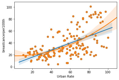
The figure below shows the fit of the linear and quadratic regression model for breast cancer per 100k and urban rate of the country.

Linear Regression Analysis:

According to the linear regression modeling (smf.ols function in python)

The linear model indicates that the P-value for urban rate is very low (0.00) indicating the null hypothesis could be rejected. i.e. there is a significant relationship between breast cancer and urban rate. One thing to note here is that R squared is 0.336 which means this linear model captures/fits 33.6% of the values.

In this case the linear regression could be modeled as follows

y = mx +b

Where,

y = breast cancer per 100k x = Urban rate m = 0.5868 b = 37.60

Quadratic Regression Analysis:

According to the quadratic regression modeling (smf.ols function in python)

The quadratic model indicates that the P-value for urban rate is very low (0.00) for the linear coefficient of urban rate and lower than 0.05 for the quadratic coefficient of urban rate indicating the null hypothesis could be rejected for this analysis. i.e. there is a significant relationship between breast cancer and urban rate.

The quadratic model fits this sample size better than the linear model. One thing to note here is that R squared is now 0.352 which means this quadratic model captures/fits 35.2% of the values. This quadratic model fits this sample better than the linear model.

In this case, the quadratic regression could be modeled as follows y = mx + m1(x^2) +b

Where y = breast cancer per 100k

x = Urban rate m = 0.6075 m1 = 0.0056 b = 34.78

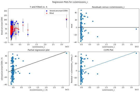
Multiple Regression Analysis:

Note: Here we add Co2 Emissions to the model check whether there is any association.

According to the multiple regression modeling (smf.ols function in python)

It could be observed that the p-value of all the coefficients urban rate, (urban rate)^2 and Co2 Emissions in this study are less than 0.05. This suggests that the null hypothesis could be rejected.

Which means, there is a significant relationship between Breast Cancer and urban rate with co2 emissions as a confounding variable.

Q-Q Plot

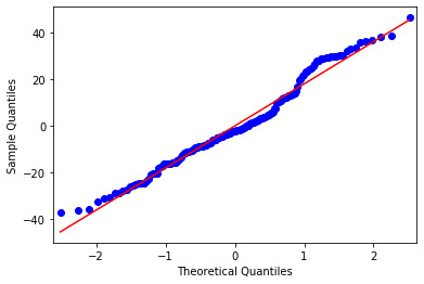
This plot shows how large the residuals are. The Straight-line in this plot indicates normally distributed residuals. In this case, the residuals do not follow a perfectly normal distribution. This could mean that the curvilinear association that we observed in our scatter plot may not be fully estimated by the quadratic urban rate term. There might be other explanatory variables that we might consider in our model to improve the estimation of observed curvilinearity.

The simple plot of Residuals:

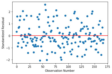
This plot shows that the most residuals lie between 2 and -2 with a few outliers.

Additional regression diagnostic plots:

leverage plot:

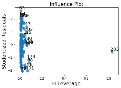
This plot shows if there are any outliers. A point with zero leverage has no effect on the regression model. In this case, the most outliers have lower leverage and value with high H leverage is not an outlier since it is close to 0. The result of this analysis could be improved by adding more explanatory variables.

Data Used:

1) The GapMinder data that includes one year of numerous country-level indicators of health, wealth and development.

https://d18ky98rnyall9.cloudfront.net/_5e80885b18b2ac5410ea4eb493b68fb4_gapminder.csv?Expires=1591747200&Signature=iXByc49QLCkuCMJLwySGjmKp0d1jopWN8HglbZ-fwUkJxtDK48zJDHK1TyLOsOENn7M-V25F4lCh7pNJe05Me~YnEnNJwGGjgmgCOl7A8BWvR1pxXHOiGUft4VKhxIyhWI8aPO9BDllXT2xecw4VVA~sjVaHGCD7wsfuL6b7ooA_&Key-Pair-Id=APKAJLTNE6QMUY6HBC5A

2) The GapMinder data Codebook

https://d396qusza40orc.cloudfront.net/phoenixassets/data-management-visualization/GapMinder%20Codebook%20.pdf

3) Python Code: # -*- coding: utf-8 -*-

"""

Created on Tue Jul 28 18:42:12 2020

@author: Saurabh

"""

import numpy

import pandas

import matplotlib.pyplot as plt

import statsmodels.api as sm

import statsmodels.formula.api as smf

import seaborn

# bug fix for display formats to avoid run time errors

pandas.set_option('display.float_format', lambda x:'%.2f'%x)

data = pandas.read_csv('C:/Users/Saurabh/Desktop/Coursera/Regression Modeling in Practice/Week 3/gapminder.csv')

# convert to numeric format

data['internetuserate'] = pandas.to_numeric(data['internetuserate'], errors='coerce')

data['urbanrate'] = pandas.to_numeric(data['urbanrate'], errors='coerce')

data['femaleemployrate'] = pandas.to_numeric(data['femaleemployrate'], errors='coerce')

data['co2emissions'] = pandas.to_numeric(data['co2emissions'], errors='coerce')

data['employrate'] = pandas.to_numeric(data['employrate'], errors='coerce')

data['alcconsumption'] = pandas.to_numeric(data['alcconsumption'], errors='coerce')

data['breastcancerper100th'] = pandas.to_numeric(data['breastcancerper100th'], errors='coerce')

data['lifeexpectancy'] = pandas.to_numeric(data['lifeexpectancy'], errors='coerce')

#data['breastcancerper100th'] = pandas.to_numeric(data['breastcancerper100th'], errors='coerce')

data['urbanrate_c'] = (data['urbanrate'] - data['urbanrate'].mean())

#sub1['internetuserate_c'] = (sub1['internetuserate'] - sub1['internetuserate'].mean())

data['co2emissions_c'] = (data['co2emissions'] - data['co2emissions'].mean())

#%%

## center quantitative IVs for regression analysis

#sub1['urbanrate_c'] = (sub1['urbanrate'] - sub1['urbanrate'].mean())

##sub1['internetuserate_c'] = (sub1['internetuserate'] - sub1['internetuserate'].mean())

#sub1['co2emissions_c'] = (sub1['co2emissions'] - sub1['co2emissions'].mean())

##sub1['breastcancerper100th_c'] = (sub1['breastcancerper100th'] - sub1['breastcancerper100th'].mean())

#sub1[["lifeexpectancy", "urbanrate_c", "co2emissions_c"]].describe()

#%%

# listwise deletion of missing values

#sub1 = data[['lifeexpectancy','urbanrate', 'femaleemployrate', 'internetuserate', 'co2emissions', 'employrate', 'alcconsumption', 'breastcancerper100th']].dropna()

sub1 = data[['breastcancerper100th','urbanrate_c', 'co2emissions_c', 'urbanrate']].dropna()

####################################################################################

# POLYNOMIAL REGRESSION

####################################################################################

# first order (linear) scatterplot

scat1 = seaborn.regplot(y="breastcancerper100th", x="urbanrate", scatter=True, data=sub1)

plt.ylabel('breastcancerper100th')

plt.xlabel('Urban Rate')

# fit second order polynomial

# run the 2 scatterplots together to get both linear and second order fit lines

scat1 = seaborn.regplot(y="breastcancerper100th", x="urbanrate", scatter=True, order=2, data=sub1)

plt.ylabel('breastcancerper100th')

plt.xlabel('Urban Rate')

#%%

# linear regression analysis

reg1 = smf.ols('breastcancerper100th ~ urbanrate_c', data=sub1).fit()

print (reg1.summary())

#%%

# quadratic (polynomial) regression analysis

# run following line of code if you get PatsyError 'ImaginaryUnit' object is not callable

#del I

reg2 = smf.ols('breastcancerper100th ~ urbanrate_c + I(urbanrate_c**2)', data=sub1).fit()

print (reg2.summary())

#%%

####################################################################################

# EVALUATING MODEL FIT

####################################################################################

# adding CO2 emissions use rate

reg3 = smf.ols('breastcancerper100th ~ urbanrate_c + I(urbanrate_c**2) + co2emissions_c',data=sub1).fit()

print (reg3.summary())

#%%

#Q-Q plot for normality

fig4=sm.qqplot(reg3.resid, line='r')

#%%

# simple plot of residuals

fig8=pandas.DataFrame(reg3.resid_pearson)

plt.plot(fig8, 'o', ls='None')

l = plt.axhline(y=0, color='r')

plt.ylabel('Standardized Residual')

plt.xlabel('Observation Number')

# additional regression diagnostic plots

fig2 = plt.figure(figsize=(12,8))

fig2 = sm.graphics.plot_regress_exog(reg3, "co2emissions_c", fig=fig2)

# leverage plot

fig3=sm.graphics.influence_plot(reg3, size=8)

print(fig3)

#regression analysis Multiple Regression Data Analysis

1 note · View note

saurabh3494 · 5 years ago

Text

Is generalized anxiety associated with alcohol consumption in adults?

In this blog, an attempt was made to fit the relation between the generalized anxiety and alcohol dependence among the individuals in a linear regression model.

Problem Set up:

Sample

Procedure

Measures

Solution:

Explanatory Variable: Alcohol Dependence (Categorical)

Response Variable: Generalized Anxiety (Categorical)

In this case the null hypothesis is

H_o = There is no relationship between the Explanatory variable and Response Variable.

And the alternative hypothesis is

H_1 = There is a relationship between the Explanatory variable and Response Variable.

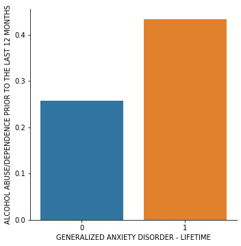
The problem is setup in such a way that if there is no alcohol dependence then it is coded as “0” and in if there is alcohol dependence/abuse observed it is coded “1”.

According to the linear regression modelling (smf.ols function in python)

It could be observed that the p value for F statistic in this study is very less than 0.05. i.e 6.11e-67. This suggests that the null hypothesis could be rejected.

Which means, there is a significant relationship between Alcohol Dependence and Generalized Anxiety.

In this case the linear regression could be modelled as follows

y = mx +b

Where

y = Generalized Anxiety

x = Alcohol Dependence

m = 0.179

b = 0.257

Generalized Anxiety = (0.179 * Alcohol Dependence) + 0.257

In summary:

Explanatory Variable: Alcohol Dependence (Categorical)

Response Variable: Generalized Anxiety (Categorical)

Result of linear regression modelling:

P value was 6.11e-67 (less than 0.05). Hence null hypothesis was rejected.

It was observed that there is a significant relationship between Alcohol Dependence and Generalized Anxiety.

Model:

Generalised Anxiety = (0.179 * Alcohol Dependence) + 0.257

Program and Data Used:

# -*- coding: utf-8 -*- """ Created on Sat Jul 25 16:24:24 2020

@author: Saurabh """

import numpy import pandas import statsmodels.api as sm import seaborn import statsmodels.formula.api as smf import matplotlib.pyplot as plt

# bug fix for display formats to avoid run time errors pandas.set_option('display.float_format', lambda x:'%.2f'%x) data = pandas.read_csv('nesarc_pds.csv', low_memory=False)

############################################################################ #DATA MANAGEMENT ############################################################################

#setting variables you will be working with to numeric data['IDNUM'] =pandas.to_numeric(data['IDNUM'], errors='coerce') data['TAB12MDX'] = pandas.to_numeric(data['TAB12MDX'], errors='coerce') data['MAJORDEPLIFE'] = pandas.to_numeric(data['MAJORDEPLIFE'], errors='coerce') #data['NDSymptoms'] = pandas.to_numeric(data['NDSymptoms'], errors='coerce') data['SOCPDLIFE'] = pandas.to_numeric(data['SOCPDLIFE'], errors='coerce') data['DYSLIFE'] = pandas.to_numeric(data['DYSLIFE'], errors='coerce') data['S3AQ3C1'] = pandas.to_numeric(data['S3AQ3C1'], errors='coerce') data['AGE'] =pandas.to_numeric(data['AGE'], errors='coerce') data['SEX'] = pandas.to_numeric(data['SEX'], errors='coerce') data['TABLIFEDX'] = pandas.to_numeric(data['TABLIFEDX'], errors='coerce') data['GENAXLIFE'] = pandas.to_numeric(data['GENAXLIFE'], errors='coerce') data['ALCABDEPP12DX'] = pandas.to_numeric(data['ALCABDEPP12DX'], errors='coerce')

#def ALCOHOLDEP (x): # if x['ALCABDEPP12DX']==0: # return 0 # else: # return 1

data.loc[data['ALCABDEPP12DX'] != 0 , 'ALCABDEPP12DX'] = 1

############################################################################ # CATEGORICAL EXPLANATORY VARIABLES ############################################################################ # depression ## modelname = smf.ols(formula='QUANT_RESPONSE ~ QUANT_EXPLANATORY', data=dataframe).fit() ## print(modelname.summary())

reg1 = smf.ols('ALCABDEPP12DX ~ GENAXLIFE', data=data).fit()

print (reg1.summary()) #%% ## listwise deletion for calculating means for regression model observations sub1 = data[['ALCABDEPP12DX', 'GENAXLIFE']].dropna()

# group means & sd print ("Mean") ds1 = sub1.groupby('GENAXLIFE').mean() print (ds1) print ("Standard deviation") ds2 = sub1.groupby('GENAXLIFE').std() print (ds2) #%% # bivariate bar graph seaborn.factorplot(x="GENAXLIFE", y="ALCABDEPP12DX", data=sub1, kind="bar", ci=None) plt.xlabel('GENERALIZED ANXIETY DISORDER - LIFETIME') plt.ylabel('ALCOHOL ABUSE/DEPENDENCE PRIOR TO THE LAST 12 MONTHS')

1) National Epidemiologic Survey of Drug Use and Health Code Book https://d396qusza40orc.cloudfront.net/phoenixassets/data-management-visualization/NESARC%20Wave%201%20Code%20Book%20w%20toc.pdf

2) National Epidemiologic Survey of Drug Use and Health Data Set https://d18ky98rnyall9.cloudfront.net/_cf16dab6c94262cc58a6bd4e0f753e56_nesarc_pds.csv?Expires=1591228800&Signature=Du9GwUu0lBCV5qy4IXbtfk09cdDXsXN5wFUmbkmBLjmuJ0chhURpBIE2CTRY8fzMoxnsvHcb3~zwEHE2GzFPjkwewqFFaGjpFxK5tGFIc7R6bKASBsQtBLqKBtpS-82JVbMcFYtfj1bPRccs~0ChboSq5PAnK02wgpZLpD7wPVM_&Key-Pair-Id=APKAJLTNE6QMUY6HBC5A

3) Introduction to the National Epidemiologic Survey on Alcohol and Related Conditions

https://pubs.niaaa.nih.gov/publications/arh29-2/74-78.htm

#Linear Regression #Data Analysis #Regression Analysis

1 note · View note

saurabh3494 · 5 years ago

Text

Is generalized anxiety associated with alcohol consumption in adults?

This blog is an example on how a regression model problem is set up. These general steps help describe data management steps to others coherently.

Sample

Procedure

Measures

In summary

Explanatory Variable: Drinking frequency (Quantitative)

Drinking quantity (Quantitative) with alcohol abuse/dependence (Categorical)

Response Variable:

Generalized Anxiety (Categorical)

Data Used:

1) National Epidemiologic Survey of Drug Use and Health Code Book https://d396qusza40orc.cloudfront.net/phoenixassets/data-management-visualization/NESARC%20Wave%201%20Code%20Book%20w%20toc.pdf

2) National Epidemiologic Survey of Drug Use and Health Data Set https://d18ky98rnyall9.cloudfront.net/_cf16dab6c94262cc58a6bd4e0f753e56_nesarc_pds.csv?Expires=1591228800&Signature=Du9GwUu0lBCV5qy4IXbtfk09cdDXsXN5wFUmbkmBLjmuJ0chhURpBIE2CTRY8fzMoxnsvHcb3~zwEHE2GzFPjkwewqFFaGjpFxK5tGFIc7R6bKASBsQtBLqKBtpS-82JVbMcFYtfj1bPRccs~0ChboSq5PAnK02wgpZLpD7wPVM_&Key-Pair-Id=APKAJLTNE6QMUY6HBC5A

3) Introduction to the National Epidemiologic Survey on Alcohol and Related Conditions https://pubs.niaaa.nih.gov/publications/arh29-2/74-78.htm

#Data Analysis Regression Modeling #regression modeling

1 note · View note

saurabh3494 · 5 years ago

Text

How are grades associated with the number of hours a student spends watching TV per week?

Here, I try to find relation between the number of hours a student spends watching TV per week vs their Grades in Mathematics. I used ANOVA (Analysis Of Variance) to support this data analysis. To take this study further, I used a moderator to check whether getting enough sleep affects this study or not.

Here I used following as my explanatory and response variables for Case 1 and Case 2:

Case 1 without moderator

Explanatory Variable: Grades (2 level Categorical, A or less)

Response Variable: Number of hours spend watching TV per week (Quantitative 0-99 hrs/week)

Case 2 with moderator

Explanatory Variable : Grades (2 level Categorical, A or less)

Moderator: Getting enough sleep (2 level Categorical, yes or no)

Response Variable: Number of hours spend watching TV per week (Quantitative 0-99 hrs/week)

Note both the Explanatory and Response variables are Quantitative.

The null hypothesis will be: H_0 : There is no relation between the explanatory and response variables.

And the alternate hypothesis will be H_a : There is relation between the explanatory and response variables.

The National Longitudinal Study of Adolescent Health (AddHealth) is a representative school-based survey of adolescents in grades 7-12 in the United States. The Wave 1 survey focuses on factors that may influence adolescents’ health and risk behaviors, including personal traits, families, friendships, romantic relationships, peer groups, schools, neighborhoods, and communities.

CASE 1 without a moderator:

Study 1.0

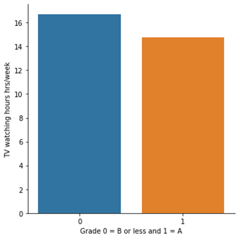
According to ANOVA test on this Data, it was found that:

The P value (1.32e-5) is significantly lower than 0.05 in which gives us significant confidence to conclude that null hypothesis can be rejected. In other words, there is a relationship number of hours spent watching TV and Getting an A in mathematics. Students spending less time watching TV scored A grade in mathematics.

Means and Standard deviations are shown above. Based on ANOVA, it could be concluded that the mean hours of watching TV 16.6 hrs/week and 14.7 hrs/week are significantly different from each other.

CASE 2:

Does getting enough sleep has anything to do with getting better grades in case 1?

Here ’getting enough sleep’ was set as a moderator to check how case 1 results affect.

Two separate studies were done to check how getting enough sleep affects the above study.

Study 2.1:

In the case where students get enough sleep, it was found that there is a relationship between the number of hours spent watching TV and Getting an A in mathematics. Students spending less time watching TV scored A grade in mathematics.

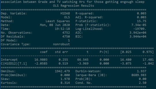
The P value (7.34e-5) is significantly lower than 0.05 in which gives us significant confidence to conclude that null hypothesis can be rejected.

Study 2.2:

In the case where students did not get enough sleep, it was found that there is no relationship between the number of hours spent watching TV and Getting an A in mathematics. Students spending less time watching TV scored A grade in mathematics.

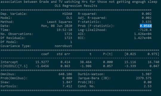
The P value (0.0568) is not significantly lower than 0.05 in which gives us significant confidence to conclude that null hypothesis accepted. i.e. there is no relationship between the Explanatory variable and Response Variable .

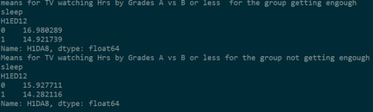
Further checking the means of both the studies (study 2.1 and study 2.2) , it could be concluded that the null hypothesis can be rejected in study 2.1 i.e. 16.9 hrs/week and 14.92 hrs/week are significantly different. Getting enough sleep has a significant effect on this study.

And

the null hypothesis can be accepted in study 2.2 i.e. there is no significant difference between 15.9 hrs/week and 14.28 hrs/week. Not getting enough sleep has no significant effect on this study.

Data Used

1) The National Longitudinal Study of Adolescent Health (AddHealth) CodeBook

https://d396qusza40orc.cloudfront.net/phoenixassets/data-management-visualization/AddHealth%20Wave%201%20Codebooks.zip

2) The National Longitudinal Study of Adolescent Health (AddHealth) Data Set:

https://d18ky98rnyall9.cloudfront.net/_e9d2d409bf11bb736eb1bd355871c3f6_addhealth_pds.csv?Expires=1591747200&Signature=adYIvJgC-qo5FTfCgmoKife3-H9wRiUvJ~jvt-8PWrz0ShXolyuxn0AIQx874gT0pJ3fpImZtm~4B4ngPCfDG3LQLrjWFvuP8GkSWUqcGqqyzurEgT21FMR53pgBgPUljrkJrnro2GPR6jPv0os8oWD-Ax-oeEZvnRLerb3mQaw_&Key-Pair-Id=APKAJLTNE6QMUY6HBC5A

3) Python CODE:

# -*- coding: utf-8 -*- """ Created on Mon Jun 8 17:36:00 2020

@author: Saurabh """

# ANOVA

import numpy import pandas import statsmodels.formula.api as smf import statsmodels.stats.multicomp as multi import seaborn import matplotlib.pyplot as plt

data = pandas.read_csv('addhealth_pds.csv', low_memory=False)

#data["H1ED12"] = data["H1ED12"].astype('category') data['H1DA8']= pandas.to_numeric(data['H1DA8'], errors='coerce')

#dir(smf) data = data[(data['H1DA8']>=0) & (data['H1DA8']<=99)] data.loc[data['H1ED12'] != 1 , 'H1ED12'] = 0

model1 = smf.ols(formula='H1DA8 ~ C(H1ED12)', data=data).fit() print (model1.summary())

sub1 = data[['H1DA8', 'H1ED12']].dropna()

print ("means for mean 'TV watching hours' by 'Grade less vs. A") m1= sub1.groupby('H1ED12').mean() print (m1)

print ("standard deviation for mean 'TV watching hours' by 'Grade less vs. A") st1= sub1.groupby('H1ED12').std() print (st1)

seaborn.factorplot(x="H1ED12", y="H1DA8", data=data, kind="bar", ci=None) plt.xlabel('Grade 0 = B or less and 1 = A') plt.ylabel('TV watching hours hrs/week')

#%% data.loc[data['H1GH52'] != 1 , 'H1GH52'] = 0 sub2=data[(data['H1GH52']== 1)] sub3=data[(data['H1GH52']== 0)]

print ('association between Grade and TV watching Hrs for those getting engough sleep') model2 = smf.ols(formula='H1DA8 ~ C(H1ED12)', data=sub2).fit() print (model2.summary())

print ('association between Grade and TV watching Hrs for those not getting engough sleep') model3 = smf.ols(formula='H1DA8 ~ C(H1ED12)', data=sub3).fit() print (model3.summary())

print ("means for TV watching Hrs by Grades A vs B or less for the group getting engough sleep") m3= sub2.groupby('H1ED12').mean() print (m3['H1DA8']) #hrs1 = m3['H1DA8'] #seaborn.factorplot(x="H1ED12", y=hrs1, data=data, kind="bar", ci=None) #plt.xlabel('Grade 0 = B or less and 1 = A') #plt.ylabel('TV watching hours hrs/week')

print ("Means for TV watching Hrs by Grades A vs B or less for the group not getting engough sleep") m4 = sub3.groupby('H1ED12').mean() print (m4['H1DA8']) #hrs2 = m4['H1DA8'] #seaborn.factorplot(x="H1ED12", y=hrs2, data=data, kind="bar", ci=None) #plt.xlabel('Grade 0 = B or less and 1 = A') #plt.ylabel('TV watching hours hrs/week')

#Data Analysis Tools #Data Analysis #ANOVA #Saurabh3494

1 note · View note

saurabh3494 · 5 years ago

Text

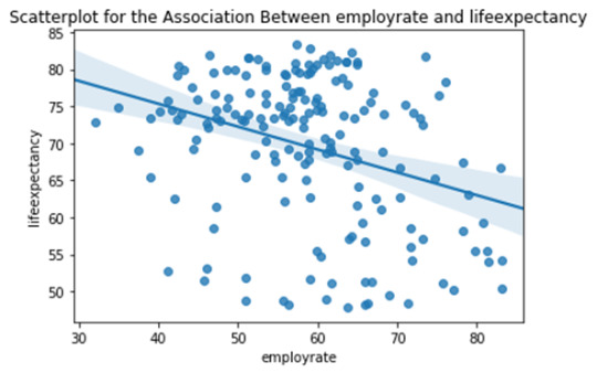
How are life expectancy and female employ rate associated with the overall employ rate of the country?

In this short study, I try to figure out relation between the life expectancy vs the overall employment rate and Female employment rate vs the overall employment rate. I used Pearson Correlation to support the data analysis.

Here I used following as my explanatory and response variables for Case 1 and Case 2:

Case 1 Explanatory Variable: overall employment rate (Quantitative)

Response Variable: Female employment rate (Quantitative)

Case 2 Explanatory Variable: overall employment rate (Quantitative)

Response Variable: life expectancy (Quantitative) Note both the Explanatory and Response variables are Quantitative.

The null hypothesis in this case will be: H_0 : There is no linear relation between the explanatory and response variables.

And the alternate hypothesis in this case will be H_a : There is linear relation between the explanatory and response variables.

GapMinder is a non-profit venture promoting sustainable global development and achievement of the United Nations Millennium Development Goals. It seeks to increase the use and understanding of statistics about social, economic, and environmental development at local, national, and global levels. The GapMinder data includes one year of numerous country-level indicators of health, wealth and development

According to Pearson Correlation on GapMinder Data, it was found that:

The P value is lower than 0.05 in both the cases which gives us significant confidence to conclude that null hypothesis can be rejected in both the cases.

Pearson ‘r’ takes value from -1 to 1. Where negative values indicate linear decremental relationship and vice versa. Values closer to 0 (Zero) indicate weak linear relationship i.e the graph will more scattered while the values closer to 1 or -1 indicate stronger linear relationship. In other words, looking at the Pearson ‘r’ values and p values of the both the cases we could conclude that

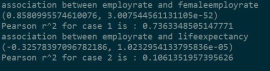
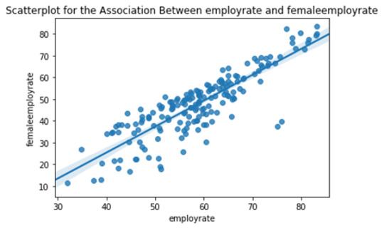
CASE1: There is a strong incremental linear relationship between the female employment rate and overall employment rate in the countries. i.e. countries having better overall employment rates tend to have better female employment rates.

CASE2: There is a moderately weak decremental linear relationship between the life expectancy and overall employment rate in the countries. i.e. countries having better overall employment rates tend to have slightly worse life expectancy.

Note: Each dot in the above scatter plots represents each country in the world.

Importance of ‘r’ value :

r^2 (r square) value indicates the fraction of variability of one variable that can be predicted by other variable.

This means that, For CASE1 : r^2 = 0.736 i.e If we know the overall employment rate of the country, we can predict 73.6% of the variability we will see in the rate of female employment.

For CASE2 : r^2 = 0.106 i.e If we know the overall employment rate of the country, we can predict only 10.6% of the variability we will see in the life expectancy.

----------------------------------------------------------------------------------------------------------

Data used:

1) The GapMinder data that includes one year of numerous country-level indicators of health, wealth and development.

2) The GapMinder data Codebook

https://d396qusza40orc.cloudfront.net/phoenixassets/data-management-visualization/GapMinder%20Codebook%20.pdf

3) Python Code

import pandas

import numpy import seaborn import scipy import matplotlib.pyplot as plt

data = pandas.read_csv('gapminder.csv', low_memory=False)

#setting variables you will be working with to numeric data['lifeexpectancy'] = pandas.to_numeric(data['lifeexpectancy'], errors='coerce') data['femaleemployrate'] = pandas.to_numeric(data['femaleemployrate'], errors='coerce') data['employrate'] = pandas.to_numeric(data['employrate'], errors='coerce')

data['employrate']=data['employrate'].replace(' ', numpy.nan)

f1 = plt.figure(1)

scat1 = seaborn.regplot(x="employrate", y="femaleemployrate", fit_reg=True, data=data) plt.xlabel('employrate') plt.ylabel('femaleemployrate')

plt.title('Scatterplot for the Association Between employrate and femaleemployrate')

f2 = plt.figure(2)

scat2 = seaborn.regplot(x="employrate", y="lifeexpectancy", fit_reg=True, data=data) plt.xlabel('employrate') plt.ylabel('lifeexpectancy') plt.title('Scatterplot for the Association Between employrate and lifeexpectancy')

plt.show()

data_clean=data.dropna()

print ('association between employrate and femaleemployrate') C1 = scipy.stats.pearsonr(data_clean['employrate'], data_clean['femaleemployrate']) print (C1) i1, i2 = C1 i1 = (i1)**2 print ("Pearson r^2 for case 1 is : {}".format(i1))

print ('association between employrate and lifeexpectancy') C2 = scipy.stats.pearsonr(data_clean['employrate'], data_clean['lifeexpectancy']) print (C2) j1, j2 = C2 j1 = (j1)**2

print ("Pearson r^2 for case 2 is : {}".format(j1))

Code output: association between employrate and femaleemployrate (0.8580995574610076, 3.007544561131105e-52) Pearson r^2 for case 1 is : 0.7363348505147771 association between employrate and lifeexpectancy (-0.32578397096782186, 1.0232954133795836e-05) Pearson r^2 for case 2 is : 0.1061351957395626

#Data Analysis Tools #Data Analysis #Pearson Correlation #Saurabh3494

1 note · View note

saurabh3494 · 5 years ago

Text

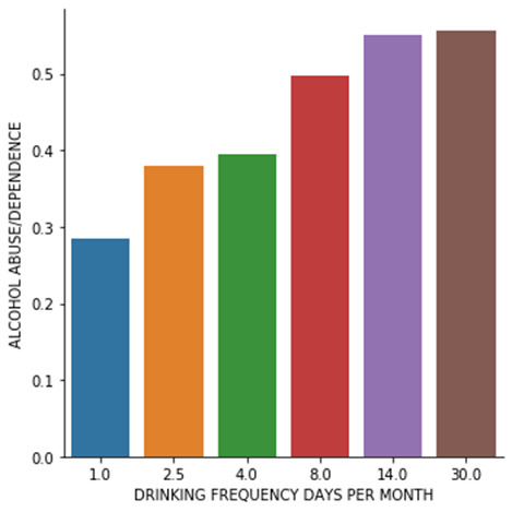
Is frequency of drinking alcohol associated with alcohol abuse/dependence among adults?

In this short study, I try to figure out whether there is relation between the frequency of drinking alcohol and alcohol abuse/alcohol dependence among adults. Here I used CHI Square Test to study the relation between the two categorical variables.

Here I used following as my explanatory and response variables:

Explanatory Variable: Drinking frequency (Categorical with 6 levels: drinking 1,2.5,4,8,14,30 days/month)

Response Variable: alcohol abuse/dependence (Categorical with 2 levels: yes, no)

The null hypothesis in this case will be: H_0 : There is no relation between the explanatory and response variables. i.e Frequency of drinking alcohol among adults is not associated with alcohol abuse/dependence.

And the alternate hypothesis in this case will be H_a : There is relation between the explanatory and response variables. (alternate hypothesis). i.e Frequency of drinking alcohol among the adults is associated with alcohol abuse/dependence.

The U.S. National Epidemiological Survey on Alcohol and Related Conditions (NESARC) is a survey designed to determine the magnitude of alcohol use and psychiatric disorders in the U.S. population. It is a representative sample of the non-institutionalized population 18 years and older.

According to Chi Square Test on NESARC survey, it was found that:

The P value (1.09e-125) is lower than 0.05 which gives us significant confidence to reject the null hypothesis. Here we accept the alternate hypothesis. In other words, looking at the chi-square value and p value in this case, it could be concluded that both the mean frequencies of alcohol consumption are significantly different in alcohol abuse/dependence case. i.e alcohol abuse/dependence and drinking is associated with each other.

POST HOC TEST FOR CHI SQUARE STUDY

Bonferroni Adjustment.

Since Explanatory variable has 6 categorical levels, the total number of paired comparisons will be 5+4+3+2+1 = 15. The Bonferroni Adjustment in this case will be p/c = 0.05/15 = 0.0033 where, p = min p value required to accept the null hypothesis and c = number of comparisons.

The pairs compared in the post HOC study are 1) 1day/month vs 2.5 days/month 2) 1day/month vs 4 days/month ..... .... ....

15) 14 days/month vs 30 days/month Pairwise P values of each Post HOC comparison is shown in the table below.

(Python code and results posted in ‘keep reading’ section below)

For two values to be significantly different, the observed P value should be smaller than adjusted Bonferroni P value of 0.0033.

It could be observed that frequency 1 day/month is significantly different than all other frequencies. The graphical illustration of all the comparisons is attempted below.

The Post HOC results could be readjusted and graphically shown as below:

-----------------------------------------------------------------------------------------------------------

Data Used:

1) National Epidemiologic Survey of Drug Use and Health Code Book https://d396qusza40orc.cloudfront.net/phoenixassets/data-management-visualization/NESARC%20Wave%201%20Code%20Book%20w%20toc.pdf

2) National Epidemiologic Survey of Drug Use and Health Data Set https://d18ky98rnyall9.cloudfront.net/_cf16dab6c94262cc58a6bd4e0f753e56_nesarc_pds.csv?Expires=1591228800&Signature=Du9GwUu0lBCV5qy4IXbtfk09cdDXsXN5wFUmbkmBLjmuJ0chhURpBIE2CTRY8fzMoxnsvHcb3~zwEHE2GzFPjkwewqFFaGjpFxK5tGFIc7R6bKASBsQtBLqKBtpS-82JVbMcFYtfj1bPRccs~0ChboSq5PAnK02wgpZLpD7wPVM_&Key-Pair-Id=APKAJLTNE6QMUY6HBC5A

3) Python CODE:

# -*- coding: utf-8 -*- """ Created on Sat Jun 6 13:48:38 2020

@author: Saurabh """

import pandas import numpy import scipy.stats import seaborn import matplotlib.pyplot as plt import itertools

data = pandas.read_csv('nesarc_pds.csv', low_memory=False) data['ALCABDEPP12DX'] = pandas.to_numeric(data['ALCABDEPP12DX'], errors='coerce') data['CONSUMER'] = pandas.to_numeric(data['CONSUMER'], errors='coerce') data['S2AQ8A'] = pandas.to_numeric(data['S2AQ8A'], errors='coerce') data['S2AQ11'] = pandas.to_numeric(data['S2AQ11'], errors='coerce') data['AGE'] = pandas.to_numeric(data['AGE'], errors='coerce')

#converting 0 ,1 ,2, 3 into 0 and 1 i.e 0 - No alcohol diagnosis and 1 - alcohol diagnosis #subset data to adults age 18 to 65 who are consumer of alcohol data.loc[data['ALCABDEPP12DX'] != 0, 'ALCABDEPP12DX'] = 1 sub1=data[(data['AGE']>=18) & (data['AGE']<=65) & (data['CONSUMER']== 1) ]

#make a copy of new subsetted data sub2 = sub1.copy()

# recode missing values to python missing (NaN) sub2['S2AQ8A']=sub2['S2AQ8A'].replace(8, numpy.nan) sub2['S2AQ8A']=sub2['S2AQ8A'].replace(9, numpy.nan) sub2['S2AQ8A']=sub2['S2AQ8A'].replace(10, numpy.nan) sub2['S2AQ8A']=sub2['S2AQ8A'].replace(11, numpy.nan) sub2['S2AQ8A']=sub2['S2AQ8A'].replace(99, numpy.nan) sub2['S2AQ11']=sub2['S2AQ11'].replace(99, numpy.nan)

#recoding values for S2AQ8A into a new variable, USFREQMO recode1 = {1: 30, 2: 30, 3: 14, 4: 8, 5: 4, 6: 2.5, 7: 1} sub2['USFREQMO']= sub2['S2AQ8A'].map(recode1)

# contingency table of observed counts ct1=pandas.crosstab(sub2['ALCABDEPP12DX'], sub2['USFREQMO']) print (ct1)

# column percentages colsum=ct1.sum(axis=0) colpct=ct1/colsum print(colpct)

# chi-square print ('chi-square value, p value, expected counts') cs1= scipy.stats.chi2_contingency(ct1) print (cs1) # # set variable types sub2["USFREQMO"] = sub2["USFREQMO"].astype('category') sub2['ALCABDEPP12DX'] = pandas.to_numeric(sub2['ALCABDEPP12DX'], errors='coerce')

# graph percent with alocohol abuse/dependence dependence within each alcohol consumption frequency group seaborn.factorplot(x="USFREQMO", y="ALCABDEPP12DX", data=sub2, kind="bar", ci=None) plt.xlabel('DRINKING FREQUENCY DAYS PER MONTH') plt.ylabel('ALCOHOL ABUSE/DEPENDENCE') #

#Paired Combination Iterations

for pair in itertools.combinations([1,2.5,4,8,14,30], 2):

int1, int2 = pair recode = {int1:int1, int2:int2 } ct=pandas.crosstab(sub2['ALCABDEPP12DX'], sub2['USFREQMO'].map(recode)) print("chi sq test of subcategory: {}".format(pair)) print (ct) colsum=ct.sum(axis=0) colpct1=ct/colsum print(colpct1) print("chi sq test of subcategory: {}".format(pair)) cs = scipy.stats.chi2_contingency(ct) print (cs) ----------------------------------------------------------------------------------------------------------- CHI SQUARE TEST RESULT: USFREQMO 1.0 2.5 4.0 8.0 14.0 30.0 ALCABDEPP12DX 0 1734 2022 1801 1335 1064 1066 1 692 1237 1172 1320 1299 1336 USFREQMO 1.0 2.5 4.0 8.0 14.0 30.0 ALCABDEPP12DX 0 0.714757 0.620436 0.605785 0.502825 0.450275 0.443797 1 0.285243 0.379564 0.394215 0.497175 0.549725 0.556203 chi-square value, p value, expected counts (591.9713868394573, 1.0977806293259079e-125, 5, array([[1361.32429407, 1828.75345192, 1668.26757059, 1489.82522702, 1325.97250902, 1347.85694738], [1064.67570593, 1430.24654808, 1304.73242941, 1165.17477298, 1037.02749098, 1054.14305262]])) POST HOC RESULTS: chi sq test of subcategory: (1, 2.5) USFREQMO 1.0 2.5 ALCABDEPP12DX 0 1734 2022 1 692 1237 USFREQMO 1.0 2.5 ALCABDEPP12DX 0 0.714757 0.620436 1 0.285243 0.379564 chi sq test of subcategory: (1, 2.5) (54.770698468039214, 1.3544517385419353e-13, 1, array([[1602.82427441, 2153.17572559], [ 823.17572559, 1105.82427441]])) chi sq test of subcategory: (1, 4) USFREQMO 1.0 4.0 ALCABDEPP12DX 0 1734 1801 1 692 1172 USFREQMO 1.0 4.0 ALCABDEPP12DX 0 0.714757 0.605785 1 0.285243 0.394215 chi sq test of subcategory: (1, 4) (69.69478952340515, 6.922873814322958e-17, 1, array([[1588.42563438, 1946.57436562], [ 837.57436562, 1026.42563438]])) chi sq test of subcategory: (1, 8) USFREQMO 1.0 8.0 ALCABDEPP12DX 0 1734 1335 1 692 1320 USFREQMO 1.0 8.0 ALCABDEPP12DX 0 0.714757 0.502825 1 0.285243 0.497175 chi sq test of subcategory: (1, 8) (237.16710978927773, 1.6308613236724482e-53, 1, array([[1465.34028735, 1603.65971265], [ 960.65971265, 1051.34028735]])) chi sq test of subcategory: (1, 14) USFREQMO 1.0 14.0 ALCABDEPP12DX 0 1734 1064 1 692 1299 USFREQMO 1.0 14.0 ALCABDEPP12DX 0 0.714757 0.450275 1 0.285243 0.549725 chi sq test of subcategory: (1, 14) (343.6361803742184, 1.0303562387865595e-76, 1, array([[1417.40405095, 1380.59594905], [1008.59594905, 982.40405095]])) chi sq test of subcategory: (1, 30) USFREQMO 1.0 30.0 ALCABDEPP12DX 0 1734 1066 1 692 1336 USFREQMO 1.0 30.0 ALCABDEPP12DX 0 0.714757 0.443797 1 0.285243 0.556203 chi sq test of subcategory: (1, 30) (362.64890146193477, 7.4610349684920965e-81, 1, array([[1406.95940348, 1393.04059652], [1019.04059652, 1008.95940348]])) chi sq test of subcategory: (2.5, 4) USFREQMO 2.5 4.0 ALCABDEPP12DX 0 2022 1801 1 1237 1172 USFREQMO 2.5 4.0 ALCABDEPP12DX 0 0.620436 0.605785 1 0.379564 0.394215 chi sq test of subcategory: (2.5, 4) (1.3461082339165986, 0.24595963457382342, 1, array([[1999.2228819, 1823.7771181], [1259.7771181, 1149.2228819]])) chi sq test of subcategory: (2.5, 8) USFREQMO 2.5 8.0 ALCABDEPP12DX 0 2022 1335 1 1237 1320 USFREQMO 2.5 8.0 ALCABDEPP12DX 0 0.620436 0.502825 1 0.379564 0.497175 chi sq test of subcategory: (2.5, 8) (81.98141569491013, 1.3737232237288822e-19, 1, array([[1849.92610754, 1507.07389246], [1409.07389246, 1147.92610754]])) chi sq test of subcategory: (2.5, 14) USFREQMO 2.5 14.0 ALCABDEPP12DX 0 2022 1064 1 1237 1299 USFREQMO 2.5 14.0 ALCABDEPP12DX 0 0.620436 0.450275 1 0.379564 0.549725 chi sq test of subcategory: (2.5, 14) (159.49488059167192, 1.4588542363941614e-36, 1, array([[1788.91390964, 1297.08609036], [1470.08609036, 1065.91390964]])) chi sq test of subcategory: (2.5, 30) USFREQMO 2.5 30.0 ALCABDEPP12DX 0 2022 1066 1 1237 1336 USFREQMO 2.5 30.0 ALCABDEPP12DX 0 0.620436 0.443797 1 0.379564 0.556203 chi sq test of subcategory: (2.5, 30) (173.31103550758314, 1.3997260876822529e-39, 1, array([[1777.74103515, 1310.25896485], [1481.25896485, 1091.74103515]])) chi sq test of subcategory: (4, 8) USFREQMO 4.0 8.0 ALCABDEPP12DX 0 1801 1335 1 1172 1320 USFREQMO 4.0 8.0 ALCABDEPP12DX 0 0.605785 0.502825 1 0.394215 0.497175 chi sq test of subcategory: (4, 8) (59.84368736597389, 1.0269822030382857e-14, 1, array([[1656.59701493, 1479.40298507], [1316.40298507, 1175.59701493]])) chi sq test of subcategory: (4, 14) USFREQMO 4.0 14.0 ALCABDEPP12DX 0 1801 1064 1 1172 1299 USFREQMO 4.0 14.0 ALCABDEPP12DX 0 0.605785 0.450275 1 0.394215 0.549725 chi sq test of subcategory: (4, 14) (127.43002159243181, 1.4958322334350576e-29, 1, array([[1596.26030735, 1268.73969265], [1376.73969265, 1094.26030735]])) chi sq test of subcategory: (4, 30) USFREQMO 4.0 30.0 ALCABDEPP12DX 0 1801 1066 1 1172 1336 USFREQMO 4.0 30.0 ALCABDEPP12DX 0 0.605785 0.443797 1 0.394215 0.556203 chi sq test of subcategory: (4, 30) (139.4246551914622, 3.55656003277558e-32, 1, array([[1585.78437209, 1281.21562791], [1387.21562791, 1120.78437209]])) chi sq test of subcategory: (8, 14) USFREQMO 8.0 14.0 ALCABDEPP12DX 0 1335 1064 1 1320 1299 USFREQMO 8.0 14.0 ALCABDEPP12DX 0 0.502825 0.450275 1 0.497175 0.549725 chi sq test of subcategory: (8, 14) (13.626977552572807, 0.00022295851672377766, 1, array([[1269.29952172, 1129.70047828], [1385.70047828, 1233.29952172]])) chi sq test of subcategory: (8, 30) USFREQMO 8.0 30.0 ALCABDEPP12DX 0 1335 1066 1 1320 1336 USFREQMO 8.0 30.0 ALCABDEPP12DX 0 0.502825 0.443797 1 0.497175 0.556203 chi sq test of subcategory: (8, 30) (17.3849257183094, 3.052372229409848e-05, 1, array([[1260.56060906, 1140.43939094], [1394.43939094, 1261.56060906]])) chi sq test of subcategory: (14, 30) USFREQMO 14.0 30.0 ALCABDEPP12DX 0 1064 1066 1 1299 1336 USFREQMO 14.0 30.0 ALCABDEPP12DX 0 0.450275 0.443797 1 0.549725 0.556203 chi sq test of subcategory: (14, 30) (0.17687528965654875, 0.6740724342219784, 1, array([[1056.28331584, 1073.71668416], [1306.71668416, 1328.28331584]]))

-----------------------------------------------------------------------------------------------------------

#data analysis tools #Chi square #chi2 #Saurabh3494

1 note · View note

saurabh3494 · 5 years ago

Text

Is gender and ethnic group associated with quantity of beer that current young adults drink?

It is claimed that males drink more beer than females. In this short study, I tried to find whether this claim is true or false. I used ANOVA (Analysis of Variance) to study how quantity of beer consumed by males and females differs. I also took this study further in determining the relation between different ethnic groups and amount of beer consumed by each of those groups.

Here I used following as my explanatory and response variables:

Explanatory Variable : Gender (Categorical) Response Variable : Beer Quantity (Quantative)

The null hypothesis in this case will be: H_0 : There is no relation between the explanatory and response variables. i.e Males and Females drink equal amount of beer. Mean amount of beer consumed by males is equal to that consumed by the females.

The alternate hypothesis in this will be H_a : There is relation between the explanatory and response variables. (alternate hypothesis). i.e Males and Females drink different amount of beer. Mean amount of beer consumed by males is not equal to that consumed by the females.

According to ANOVA F Test on NESARC survey, it was found that:

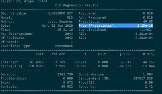
P value of the F statistic is lower than 0.05 which gives us confidence to conclude that null hypothesis could be rejected. In other words, looking at the means and standard deviations of the both the groups (1. males and 2. females) it could be concluded that both the means are not equal i.e males in fact drink more beers than females. It could be concluded that mean amount of beers consumed by Males is greater than mean amount of beers consumed by Females by 19 beers per month.

Another study was done to understand the relation between the ethnic groups and amount of beers consumed.

Is Ethnicity associated with the quantity of beer consumed?

Here, the null hypothesis will be:

H_0 : There is no relation between the explanatory and response variables. i.e all ethnic groups drink equal amount of beer. Mean amount of beer consumed by all the ethnic groups is equal.

Here I took Explanatory Variable : Ethnicity (Categorical) Response Variable : Beer Quantity (Quantative)

Running ANOVA test we get the following results.

Such low value of Prob (F-Statistic) shows that the null hypothesis could be rejected. i.e the amount of beer consumed in different ethnic groups is different.

Using Tukey HSD post HOC test it could be concluded that

Group 3 drinks most number of beers than all other ethnic groups.

The mean beer consumption between the other ethnic groups could be assumed to be equal.

Post HOC Test results are shown below.

Data used:

1) National Epidemiologic Survey of Drug Use and Health Code Book https://d396qusza40orc.cloudfront.net/phoenixassets/data-management-visualization/NESARC%20Wave%201%20Code%20Book%20w%20toc.pdf

2) National Epidemiologic Survey of Drug Use and Health Data Set https://d18ky98rnyall9.cloudfront.net/_cf16dab6c94262cc58a6bd4e0f753e56_nesarc_pds.csv?Expires=1591228800&Signature=Du9GwUu0lBCV5qy4IXbtfk09cdDXsXN5wFUmbkmBLjmuJ0chhURpBIE2CTRY8fzMoxnsvHcb3~zwEHE2GzFPjkwewqFFaGjpFxK5tGFIc7R6bKASBsQtBLqKBtpS-82JVbMcFYtfj1bPRccs~0ChboSq5PAnK02wgpZLpD7wPVM_&Key-Pair-Id=APKAJLTNE6QMUY6HBC5A

3) Python CODE:

import numpy

import pandas

import statsmodels.formula.api as smf

import statsmodels.stats.multicomp as multi

data = pandas.read_csv('nesarc_pds.csv', low_memory=False)

#setting variables you will be working with to numeric

data['S2AQ5B'] = pandas.to_numeric(data['S2AQ5B'], errors='coerce')

data['S2AQ5D'] = pandas.to_numeric(data['S2AQ5D'], errors='coerce')

data['S2AQ5A'] = pandas.to_numeric(data['S2AQ5A'], errors='coerce')

#subset data to young adults age 18 to 25 who have drank beers in the past 12 months

sub1=data[(data['AGE']>=18) & (data['AGE']<=25) & (data['S2AQ5A']==1)]

#SETTING MISSING DATA

sub1['S2AQ5B']=sub1['S2AQ5B'].replace(99, numpy.nan)

sub1['S2AQ5B']=sub1['S2AQ5B'].replace(8, numpy.nan)

sub1['S2AQ5B']=sub1['S2AQ5B'].replace(9, numpy.nan)

sub1['S2AQ5B']=sub1['S2AQ5B'].replace(10, numpy.nan)

sub1['S2AQ5D']=sub1['S2AQ5D'].replace(99, numpy.nan)

#recoding number of days drank beer in the past month

recode1 = {1: 30, 2: 30, 3: 14, 4: 8, 5: 4, 6: 2.5, 7: 1}

sub1['USFREQMO']= sub1['S2AQ5B'].map(recode1)

#converting new variable USFREQMMO to numeric

sub1['USFREQMO']= pandas.to_numeric(sub1['USFREQMO'], errors='coerce')

# Creating a secondary variable multiplying the days drank beer/month and the number of beers/per day

sub1['NUMBEERMO_EST']=sub1['USFREQMO'] * sub1['S2AQ5D']

sub1['NUMBEERMO_EST']= pandas.to_numeric(sub1['NUMBEERMO_EST'], errors='coerce')