#Linear Regression

[detrasdeldataset]

DESCIFRANDO LA RELACIÓN ENTRE INGRESOS Y CONSUMO DE ALCOHOL: EL MISTERIO DEL COEFICIENTE DE CORRELACIÓN DE PEARSON

En esta entrada, exploraremos el coeficiente de correlación de Pearson, centrándonos en la relación entre el ingreso total anual y el consumo total anual estimado de alcohol.

Análisis de los Datos

Comenzamos creando una copia de nuestro conjunto de datos y eliminando las filas con entradas NaN, ya que el coeficiente de correlación no puede calcularse con datos faltantes.

Luego, procedimos a realizar un diagrama de dispersión de estas variables.

Observamos que el comportamiento de las variables no es lineal; de hecho, parece más apropiado considerar un ajuste logarítmico para establecer una regresión entre ellas. Este será un tema que exploraremos en futuras entradas del blog.

Resultados del Análisis

Tras la realización del diagrama de dispersión, calculamos el coeficiente de correlación de Pearson.

El resultado obtenido fue un coeficiente de aproximadamente -0.015 (-0.014984230083466107), con un valor p significativo de 0.022912246058339945.

Además, el coeficiente de determinación asociado fue de 0.0002245271511942507, indicando que una fracción extremadamente baja de la variabilidad del consumo total anual de alcohol puede explicarse por el ingreso total anual.

Conclusión

Este análisis revela una correlación negativa débil entre el ingreso total anual y el consumo total anual estimado de alcohol. Sin embargo, el coeficiente de determinación sugiere que el ingreso total anual es un predictor poco confiable del consumo de alcohol, ya que explica solo una pequeña fracción de la variabilidad observada en los datos.

[imarticusblog]

Linear Regression: Definition, Types, Examples 

Linear regression has been used extensively in multiple industries for prediction purposes. This article aims to cover the definition of linear regression and types of linear regression with examples for better understanding.

[chess-dreams]

I'm learning about linear regression so I can learn about gradient descent so I can use texel tuning on my evaluation function. Linear regression sure is satisfying to watch.

[vivekavicky12]

Decoding the Enigma: Exploring Methods in Data Science Algorithms

In the ever-evolving landscape of data science, algorithms act as the essential backbone, orchestrating the intricate transformation of raw data into actionable insights. Recognizing their pivotal role, especially for those navigating the complexities of data science, this blog aims to demystify the intricate world of algorithms. Throughout this exploration, it seeks to empower readers, including those interested in a Data Science Course in Coimbatore, with a nuanced understanding of data science methods, enabling them to fully leverage the potential of algorithms in unraveling mysteries within vast datasets.

Foundations of Data Science Algorithms

Algorithms function as intricate recipes, guiding the transformation of raw data into actionable insights. This exploration delves into their fundamental definition, emphasizing their pivotal role in shaping the data science landscape. These systematic procedures decode the complexities of data and play a crucial role in guiding decision-making, empowering data scientists to extract meaningful patterns from intricate datasets.

Importance of Algorithm Selection

Choosing the appropriate algorithm mirrors the precision of selecting the perfect tool for a specific task. This exploration delves into the significance of algorithm selection, underscoring its impact on effective problem-solving across diverse domains. Just as the right tool optimizes efficiency and accuracy, judiciously choosing algorithms determines the success of analytical solutions in the broader data science landscape.

Key Concepts

Effectively navigating the expansive realm of data science algorithms requires a profound grasp of fundamental concepts, including training models, rigorous testing procedures, and comprehensive model evaluation techniques. These foundational elements serve as the bedrock for successful algorithm implementation, ensuring accuracy, efficiency, and relevance in transforming raw data into meaningful insights.

Typical algorithms in data science

Typical data science algorithms, ranging from supervised to unsupervised learning and reinforcement learning, play a pivotal role in extracting meaningful patterns from vast datasets. This array of algorithms forms the backbone of data science applications, tailored to specific tasks and scenarios, collectively empowering data scientists to tackle a wide spectrum of challenges in data analysis, prediction, and decision-making.

Algorithmic Techniques and Approaches

Algorithmic techniques and approaches enhance the performance and versatility of data science models. Utilizing ensemble methods like bagging and boosting amplifies predictive accuracy, while feature engineering and selection impact model efficiency. Cross-validation techniques ensure robust model validation, contributing to adaptability across diverse datasets.

Selecting the Right Algorithm for the Task

Choosing the most suitable algorithm involves careful consideration of factors like data nature, analysis goals, and available computational resources. This pivotal step empowers data scientists to tailor their approach, maximizing efficiency and relevance for successful data-driven projects.

Practical Examples and Case Studies

Exploring practical examples and case studies within a Data Science Course Online provides a hands-on perspective, bridging theoretical knowledge with real-world application. Participants gain insights into problem-solving and decision-making nuances, illustrating algorithm versatility across industries and their transformative impact on real-world scenarios.

Future Trends in Data Science Algorithms

Anticipating groundbreaking developments, future trends in data science algorithms incorporate artificial intelligence and machine learning seamlessly. These innovations promise enhanced predictive capabilities and improved interpretability, shaping the next frontier of data science with algorithms poised to revolutionize insights extraction from complex datasets.

This blog extensively delves into the algorithms of data science, uncovering their crucial role in transforming unprocessed data into practical insights. It simplifies the complex realm of algorithms, offering readers a nuanced comprehension of methods in data science. Encompassing fundamentals, the selection of algorithms, and essential concepts, it breaks down prevalent algorithms and investigates methods for optimizing performance. The narrative underscores the vital importance of choosing the appropriate algorithm, supported by real-world examples. Wrapping up with future trends, it anticipates the integration of AI and machine learning, heralding revolutionary progress in data science algorithms for enhanced predictability and interpretability.

[analyticsvidhya]

D/W Logistic regression vs linear regression

Linear Regression: Linear Regression models the relationship between a dependent variable and one or more independent variables. It's used for predicting continuous values, such as sales or prices.

Logistic Regression: Logistic Regression is used for binary classification problems, estimating the probability that an instance belongs to a particular category. It's common in tasks like spam detection or predicting customer purchases.

[bobbyfiend]

I think you might be stupid

ooh, anonymous! I always give great weight to insults from anonymous assholes. Such courage. Such wisdom. Such bravery.

[emergingindiaanalyticsnoida]

Step-By-Step Guide: Implementing Linear Regression For Machine Learning

Are you ready to unravel the secrets of linear regression and unlock its potential in machine learning? Look no further! In this step-by-step guide, we will take you on an exhilarating journey through the world of linear regression. Whether you’re a beginner or an experienced data scientist, get ready to dive deep into the concepts, techniques, and practical implementation of one of the most fundamental algorithms in predictive analytics. So fasten your seatbelts and prepare to soar high as we unveil the power of linear regression for machine learning!

Introduction to Linear Regression

Linear regression is a powerful statistical technique that can be used to predict future values of a dependent variable, based on past values of an independent variable. In machine learning, linear regression can be used to build predictive models to find relationships between features and labels.

In this guide, we will go over the basics of linear regression and show how to implement it in Python. We will also cover some important considerations when working with linear regression models.

What is Linear Regression?

Linear regression is a statistical technique that can be used to predict future values of a dependent variable, based on past values of an independent variable. In machine learning, linear regression can be used to build predictive models to find relationships between features and labels.

Independent variables are typically denoted by X while the dependent variable is denoted by Y . For example, in our housing price dataset, the feature X could represent the size of the house (in square feet) while the label Y could represent the price of the house. We would then want to find a relationship between X and Y so that we can predict prices given only the size of the house. This relationship is typically represented by a line:

Y = mX + b

where m is the slope of the line and b is the intercept (the value of Y when X=0). The goal of linear regression is to estimate the values for m and b so that we can best fit this line to our

Preparing Data for Linear Regression

In machine learning, linear regression is a supervised learning algorithm used to predict a continuous target variable y from a set of predictor variables X. The goal is to find the best fit line that describes the relationship between the predictor variables and the target variable.

To prepare data for linear regression, you need to ensure that your data is free of missing values and outliers, and that it is properly scaled. You also need to split your data into training and test sets, so that you can assess the performance of your linear regression model on unseen data.

Once your data is ready, you can begin fitting a linear regression model using scikit-learn or another machine learning library. Be sure to tune your model hyperparameters to get the best possible performance on your test set.

Implementing Linear Regression in Machine Learning

Linear regression is a machine learning algorithm that can be used to predict continuous values. In this guide, we will go over how to implement linear regression in machine learning. We will cover the following topics:

– What is linear regression?

– The mathematical equation for linear regression

– How to implement linear regression in machine learning

– Tips for improving your linear regression model

What is linear regression?

Linear regression is a machine learning algorithm that is used to predict continuous values. Continuous values are numerical values that can take any value within a certain range. Examples of continuous values include height, weight, and temperature. Linear regression predicts the value of a target variable by using a line of best fit. The line of best fit is created by finding the line that minimizes the sum of squared errors.

The mathematical equation for linear regression

The mathematical equation for linear regression is y =mx+b, where y is the predicted value, m is the slope of the line, x is the input value, and b is the intercept. The slope and intercept are learned by the algorithm during training.

How to implement linear regression in machine learning

Linear regression can be implemented in many different programming languages. In this guide, we will show you how to implement linear regression in Python. First, we will need to import the libraries that we will be using:

from sklearn import datasets  # To load our dataset

from sklearn import

Learning Algorithms and Models Used in Linear Regression

There are a few different types of learning algorithms and models that can be used for linear regression. The most common type of algorithm is the Ordinary Least Squares (OLS) estimator. This method finds the line of best fit by minimizing the sum of squared residuals. Another popular algorithm is the gradient descent algorithm. This approach starts with a randomly generated line and then iteratively improves it by moving it in the direction that minimizes the cost function. There are also many different ways to regularize linear regression models to prevent overfitting, such as adding L1 or L2 regularization terms to the cost function.

Evaluating Performance of Linear Regression Models

It is important to evaluate the performance of your linear regression models to ensure that they are accurately predicting outcomes. There are a few key metrics that you can use to evaluate your model’s performance, including:

-R Squared: This metric measures the percentage of variability in the dependent variable that is explained by the independent variable(s). A high R squared value indicates a strong relationship between the independent and dependent variables.

-Mean Absolute Error: This metric measures the average difference between predicted values and actual values. A low MAE value indicates that the model is accurately predicting outcomes.

-Root Mean Squared Error: This metric measures the average difference between predicted values and actual values, taking into account the magnitude of the error. A low RMSE value indicates that the model is accurately predicting outcomes.

Optimization Techniques Used for Linear Regression

There are a few different ways to optimize linear regression for machine learning. The first is to use feature selection techniques in order to choose the most predictive features for your model. This can be done using methods like forward selection, backward elimination, or recursive feature elimination. Another way to optimize linear regression is by using regularization methods like Lasso or Ridge regression. These methods help to prevent overfitting by penalizing certain coefficients in the model. You can also use cross-validation to tune your model and improve its performance.

Conclusion

Linear regression is an important algorithm that is used to solve a wide variety of machine learning problems. It offers great insight into the relationships between two or more variables and can be implemented in various ways depending on your dataset and problem requirements. We have provided you with a step-by-step guide to implement linear regression for machine learning, which we hope will help you get started quickly and achieve better results. With this knowledge under your belt, it’s time to start exploring different datasets and applying linear regression techniques to them!

[trendingnow3-blog]

Understanding Machine Learning Models for Stock Price Forecasting with Python

In this comprehensive article, we, as proficient SEO experts and adept copywriters, will explore the fascinating realm of machine learning models designed to forecast stock prices using Python. Our objective is to provide valuable insights and detailed knowledge that will outperform competing websites on Google, establishing this article as the go-to resource for understanding this intricate…

[freeudemycoursesfree]

Linear Regression and Logistic Regression using R Studio

Linear Regression and Logistic Regression using R Studio

Linear Regression and Logistic Regression for beginners. Understand the difference between Regression & Classification What you’ll learn Learn how to solve real life problem using the Linear and Logistic Regression techniquePreliminary analysis of data using Univariate and Bivariate analysis before running regression analysisGraphically representing data in R before and after analysisHow to do…

[tvareta]

Multiple Regression using R

Introduction:

Multiple regression is a branch of linear regression which can be used to analyse more than two variables. In multiple regression there is one response and more than one predictor variables whereas in linear regression where one response variable and one predictor variable. The predicator variables are the dependent variables and the response variable are the independent variables. Considering the equation for multiple regression,

Y=mx1+mx2+mx3=b

Where Y is the response variable

m1, m2, m3 are predictor variables

Let us discuss two problems regarding multiple regression

Analysis using R:

Multiple regression using R is one of the widely and often used method which is easy to use and handle.

DATA SET USED:

· https://github.com/grantgasser/Complete-Multiple-Regression

Using this dataset, we study of the relation between degree of brand liking (Y) and moisture content (X1) and sweetness (X2) of the product, the following results were obtained from the experiment based on a completely randomized design.

Some of the steps which we has to be followed are

1. Load and view the dataset

2. Identifying the data linearity in R

3. Plotting the graph

4. Implementation of Multiple Regression

5. Prediction and Interpretation

Brand Preference:

In a small-scale experimental study of the relation between degree of the brand liking (Y) and moisture content (XI) and sweetness (X2) of the product, the following results were obtained from the experiment based on a completely randomized design (data are coded:)

Analyzation of the data:

Scatter plot:

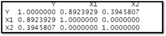
The diagnostic aids show that firstly, there are no outliers and the distribution for each variable is normal. Additionally, looking at the correlation matrix, Y and X1 have significant positive correlation, Y and X2 are positively correlated, but less so than Y and X1 and there’s no correlation between X1 and X2.

Correlation Matrix:

The correlation matrix of the variables is plotted to check the correlation between the variables.

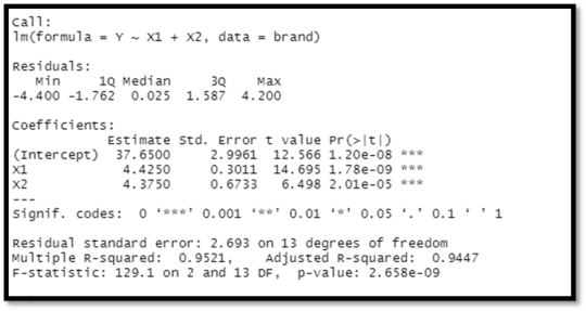
Summary:

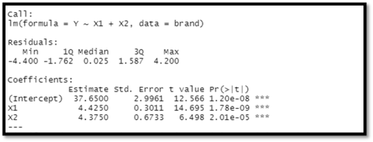
The value of multiple R- squared is 0.9521 and the adjusted R- squared value is 0.9447. When the variable X2, is added to X1 we get a p-value of about 2.01e-05. F- statistic variable is larger than 1. Y= 37.65 + 4.425X1 + 4.375X2 is the result of the regression model. Holding the other variables constant, increasing one unit of X1 results in a 4.425 rise in brand liking degree, while increasing one unit of X2 results in a 4.375 increase in brand liking degree. Because the P values for each variable are less than 0.05, both X1 and X2 are significant.

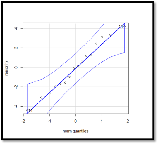
QQ plot:

In this QQ- plot the points plotted all fall in the same line which clearly determines that the residuals follow normal distribution. There are no outliers and errors .

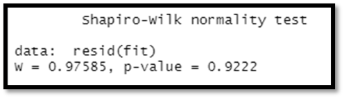
Shapiro test:

Shapiro Wilk test is a statistic normality test for a random data set. It can be used to analyse if the data set is normally distributed. By analysing the values, we get,

Model validation:

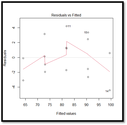
Regression vs Residual Plot:

The above given plot is a residual plot which indicates a pattern in the residuals and the fitted plot. Although the distribution appears to be pretty normal, there are outliers on both sides of the median, with more outliers to the right.

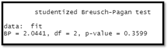
Breusch-Pagan test:

This is test can be used to determine whether the heteroscedasticity is present in a regression analysis

Prediction and Confidence level:

newX = data. frame (X1=newX1, X2 = newX2)

#Confidence interval (95%)

predict (fit, newX, interval="confidence")

#Prediction Interval (95%)

predict (fit, newX, interval="prediction"

Output:

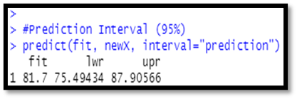
Interpretation:

From the above analysis, we get that the R- square is about 95% is very good and the results are accurate and the overall relationship is significant.

[nikimalar]

Multiple Linear Regression using R

Linear Regression

The relation between a dependent and an independent variable can be seen or predicted using linear regression models. When two or more independent variables are employed in a regression analysis, the model is referred to as a multiple regression model rather than a linear model.

Simple linear regression is a technique for predicting the value of one variable from the value of another. With linear regression, the relationship between the two variables is represented as a straight line.

In multiple regression, a dependent variable has a linear relationship with two or more independent variables. The dependent and independent variables may not follow a straight line if the relationship is non-linear.

When two or more variables are used to track a response, linear and non-linear regression are used. The non-linear regression is based on trial-and-error assumptions and is comparatively difficult to implement.

 Multiple Linear Regression

Multiple linear regression is a statistical analysis technique that uses two or more factors to predict a variable's outcome. It is also known as multiple regression and is an extension of linear regression. The dependent variable is the one that has to be predicted, and the factors that are used to forecast the value of the dependent variable are called independent or explanatory variables.

 Analysts can use multiple linear regression to determine the model's variance and the relative contribution of each independent variable. There are two types of multiple regression: linear and non-linear regression.

 Multiple Regression Equation

The equation for multiple regression with three predictor variables (x) predicting variable y is as follows:

 Y = B0 + B1 * X1 + B2 * X2 +B3 * X3

The beta coefficients are represented by the "B" values, which are the regression weights. They are the correlations between the predictor and the result variables.

Yi is predictable variable or dependent variable

B0 is the Y Intercept

B1 and B2 the regression coefficients represent the change in y as a function of a one-unit change in x1 and x2, respectively.

 Multiple Linear Regression Assumptions

        I.            The Independent Variables are not Much Correlated

Multicollinearity, which occurs when the independent variables are highly correlated, should not be present in the data. This will make finding the specific variable that contributes to the variance in the dependent variable difficult.

    II.            Relationship Between Dependent and Independent Variables

Each independent variable has a linear relationship with the dependent variable. A scatterplot is constructed and checked for linearity to check the linear relationships. If the scatterplot relationship is non-linear, the data is transferred using statistical software or a non-linear regression is done.

 III.            Observation Independence

The observations should be of each other, and the residual values should be independent. The Durbin Watson statistic works best for this.

 Multiple Linear Regression in R

Analyzing the linear relationship between Stock Index Prices and Unemployment rate in the Economy.

Multiple linear regression can be done in a variety of methods, although statistical software is the most popular. R, a free, powerful, and easily accessible piece of software, is one of the most widely used. We'll start by learning how to perform regression with R, then look at an example to make sure we understand everything.

 Steps to Apply Multiple Linear Regression in R

Step 1: Data Collection

The data needed for the forecast is gathered and collected. The purpose is to use two independents

·         Unemployment Rate

·         Interest Rate

to forecast the stock index price (the dependent variable) of a fictional economy.

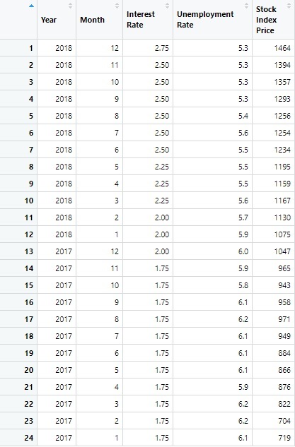
Step 2: Capturing the Data in R

Data Capturing using the code in R and Importing Excel file from save folder.

Step 3: Checking Data Linearity with R

It is critical to ensure that the dependent and independent variables have a linear relationship. Scatter plots or R code can be used to do this. Scatter plots are a quick technique to check for linearity. We need to make sure that various assumptions are met before using linear regression models. Most importantly, you must ensure that the dependent variable and the independent variable(s) have a linear relationship.

In this we'll check the Linear Relationship exist between:

·         Stock Index Price (Dependent Variable) and Interest Rate (Independent Variable)

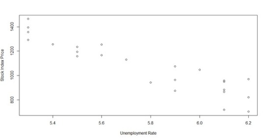
·         Stock Index Price (Dependent Variable) and Unemployment Rate (Independent Variable)

Below is the code that is used in R to plot the relations between the dependent variable that is Stock Index Price and Interest Rate.

From the Graph we can notice that there is Indeed a Linear relationship exist between the dependent variable Stock Index Price and Independent variable Interest Rate.

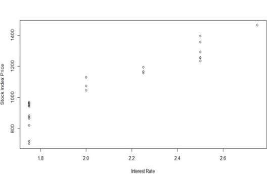
In can be specifically noted that When interest rates rise, the price of the stock index rises as well.

In the second scenario, we can plot the link between the Stock Index Price and the Unemployment Rate using the code below:

As you can see, the Stock Index Price and the Unemployment Rate have a linear relationship: when unemployment rates rise, the stock index price drops. we still have a linear correlation, although with a negative slope.

Step 4: Perform Multiple Linear Regression In R

To generate a set of coefficients, use code to conduct multiple linear regression in R. Template to perform Multiple Linear Regression in R is as below:

M1 <- lm (Dependent Variable ~ First Independent Variable + Second Independent Variable, Data= X)

Summary (M1)

Using the Template, the Code follows:

We will get the following summary if you execute the code in R:

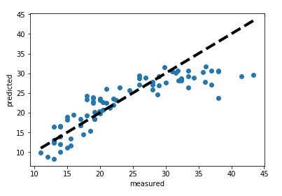
The model's residuals ('Residuals'). The model fulfils heteroscedasticity assumptions if the residuals are roughly centered around zero and have similar spread on both sides (median -6.248, and min and max -158.2 and 118.8). The model's regression coefficients ('Coefficients').

To construct the multiple linear regression equation, utilize the coefficients from the summary as follows:

Stock Index Price = (Intercept) + (Interest Rate) X1* (Unemployment Rate) X2

Once you've entered the numbers from the summary: 

Stock Index Price = (1798.4) + (345.5) X1 * (-250.1) X2

Adjusted R-squared: Measures the model's fit, with a higher number indicating a better fit.

The p-value is Pr(>|t|):  Statistical significance is defined as a p-value of less than 0.05.

Step 5: Make Predictions

 To predict the Stock Index Price from the collected Data it is noted that,

X1 <= Interest Rate = 1.5

X2 <= Unemployment Rate = 5.8

And when this data in equated into the regression Equation we obtain:

Stock Index Price = (1798.4) + (345.5) * (1.5) + (-250.1) * (5.8)

Stock Index Price = 866.066666

 The Final Predicted data for the stock Index Price using Multiple Linear Regression is 866.07.

Conclusion

The stock market and our economy's relationship frequently converge and diverges from one another. The gross domestic product, unemployment, inflation, and a slew of other indicators all represent the state of the economy. These trends are expected to show the economy and markets moving in lockstep in the long run.

When the unemployment rate is high, the Monetary Policy lowers the interest rate, which causes stock market prices to rise.

Unemployment increases often signify a drop in interest rates, which is good for stocks, as well as a drop in future corporate earnings and dividends, which is bad for stocks. Therefore, it is notable that Interest rate and Unemployment rate affect the stock market prices in the economy and have a linear relationship between the variables.