#ANOVA

[alice344]

I idk, I like art kaatie

[a-horrendous-floweroftrees]

I drew these two because I love their designs and want to know more about them.

I tried my best on the backgrounds I know it's bad lol

[rei-makes-big-robo]

Gex

[ringo-ro]

I really dont know if i wanna finish this

Anova by A3DGhost on twitter!

[pialexx]

[myfavouritepokemoncentre]

If the pokemon games keep thanos'ing the national dex. We might end up being able to get every pokemon in plush form, before being able to get them in one of the games.

[eduardotleite]

ANOVA Analysis

This is the task of Week 1 of the course Data Analysis Tools at the Coursera Plataform. The challenge is to execute an Analysis of Variance using the ANOVA Statistical Test. This type of analysis assesses whether the means of two or more groups are statistically different from each other. Is used whenever you want to compare the means (quantitative variables) of groups (categorical variables). The null hypothesis is that there is no difference in the mean of the quantitative variable across groups (categorical variable), while the alternative is that there is a difference.

DataSet Used – Gap Minder Gapminder identifies systematic misconceptions about important global trends and proportions and uses reliable data to develop easy to understand teaching materials to rid people of their misconceptions. Gapminder is an independent Swedish foundation with no political, religious, or economic affiliations. should visit it: https://www.gapminder.org/.

The dataset used has 16 variables and 213 rows. I choosed to analyze income per person (incomeperperson) and life expectancy (lifeexpectancy).

And how is the Question?

Is the life expectancy different among four categories of income per person (A,B,C,D,E)?

Since the income per person is a quantitative variable, I transformed it into a categorical variable, using parameters sugested by IBGE to classify the social class of according of income. For the parameters, I analyzed the boxplot posted below.

the data in image is in portuguese, because the IBGE is an Brazilian institute.

The Code

I used the Anaconda to code in Python for this task. The code is posted below.

import numpy import pandas as pd import statsmodels.api as sm import statsmodels.formula.api as smf import statsmodels.stats.multicomp as multi import matplotlib.pyplot as plt import seaborn as sns import researchpy as rp import pycountry_convert as pc

df = pd.read_csv('gapminder.csv') df = df[['lifeexpectancy', 'incomeperperson']]

df['lifeexpectancy'] = df['lifeexpectancy'].apply(pd.to_numeric, errors='coerce') df['incomeperperson'] = df['incomeperperson'].apply(pd.to_numeric, errors='coerce')

def income_categories(row): if row["incomeperperson"]>15000: return "A" elif row["incomeperperson"]>5000: return "B" elif row["incomeperperson"]>3000: return "C" elif row["incomeperperson"]>1000: return "D" else: return "E"

df=df[(df['lifeexpectancy']>=1) & (df['lifeexpectancy']<=120) & (df['incomeperperson'] > 0) ]

df["Income_category"]=df.apply(income_categories, axis=1)

df = df[["Income_category","incomeperperson","lifeexpectancy"]].dropna()

df["Income_category"]=df.apply(income_categories, axis=1)

print (rp.summary_cont(df['lifeexpectancy']))

fig1, ax1 = plt.subplots() df_new = [df[df['Income_category']=='A']['lifeexpectancy'], df[df['Income_category']=='B']['lifeexpectancy'], df[df['Income_category']=='C']['lifeexpectancy'], df[df['Income_category']=='D']['lifeexpectancy'], df[df['Income_category']=='E']['lifeexpectancy']] ax1.set_title('life expectancy') ax1.boxplot(df_new) plt.show()

results = smf.ols('lifeexpectancy ~ C(Income_category)', data=df).fit() print (results.summary())

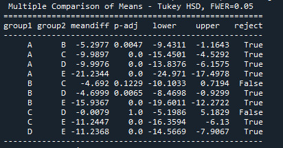
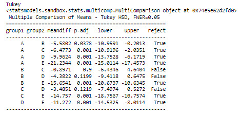
print ("Tukey") mc1 = multi.MultiComparison(df['lifeexpectancy'], df['Income_category']) print (mc1) res1 = mc1.tukeyhsd() print (res1.summary())

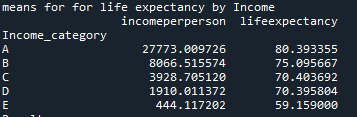
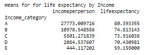
print ('means for for life expectancy by Income') m1= df.groupby('Income_category').mean() print (m1)

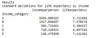
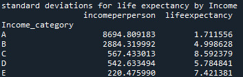
print ('Results') print ('standard deviations for life expectancy by Income') sd1 = df.groupby('Income_category').std() print (sd1)

Results – ANOVA Analysis

Aiming to answer the question of the task, I ran a test ANOVA. As shown below, from the 176 rows, 171 were used for the test, i have used a filter to remove some wrong values, as non numeric, negative, etc, reducing the rows of the original dataset

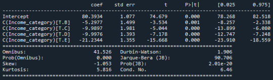
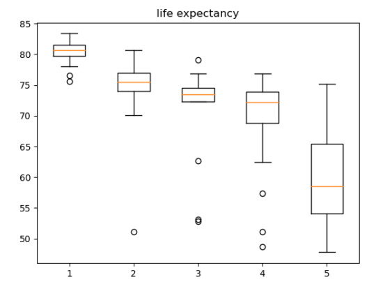
The ANOVA analysis shows a graph for each category (above) and, as we can see, the life expectancy of A class, have the life expectative of 80.39 years while the E class have the life expectative of 59.15 years.

[guailanchai]

Analysis of variance

Hypothesis testing with Analysis of Variance (ANOVA) in your course. Here's a breakdown of what you need to focus on:

Key Steps: Review Your Data Set: Ensure you have a quantitative variable (e.g., income, age, score) and a categorical variable (e.g., gender, education level). If your research question doesn't have these directly, you can: Use a quantitative variable from your data set for practice. Categorize a continuous (quantitative) variable into groups. For example, age can be grouped into ranges (20-29, 30-39, etc.). Formulate Hypotheses: Null Hypothesis (H₀): There is no significant difference between the group means. Alternative Hypothesis (H₁): There is a significant difference between the group means. ANOVA Test: ANOVA compares the mean values between groups and checks if the differences are statistically significant. If the p-value is below a certain threshold (commonly 0.05), you reject the null hypothesis, suggesting that there are statistically significant differences between the means of the groups. Example: Quantitative Variable: Exam score Categorical Variable: Study method (Group A: traditional study, Group B: online study, Group C: mixed method) Software/Tool: You can perform ANOVA using statistical software (e.g., R, Python, SPSS, Excel) or even specific web tools. Once you've run the analysis, you can interpret the results, particularly the p-value and F-statistic, to conclude whether the group means differ significantly.

[dataanalysistoolsca]

Running an analysis of variance

CODE:

OUTPUT:

[writingtree]

Get our PhD Thesis Writing Support and Services for Data Analysis by Anova, Manova, and Ancova.

Here are some benefits:

1. Expertise and Knowledge

2. Accurate and Valid Results

3. Time and Effort Saving

4. Interpretation and Discussion

5. Formatting and Presentation

6. Quality Assurance

www.writingtree.in

wa.me/+916264689448

sales.writingtree@gmail.com

Contact Now!

Our services provide help at various stages of your thesis writing process, from topic selection and proposal development to the final thesis submission.

[mars-crater]

ANOVA

La prueba ANOVA se realiza cuando nuestra variable explicativa es categórica y la variable de respuesta es cuantitativa. En este caso, ambas variables son cuantitativas, por lo que categorizamos la variable explicativa para poder realizar la prueba ANOVA.

¿Existe relación entre el diámetro de los cráteres de marte clasificados por cuartiles y la profundidad de los mismos?

Nuestras hipótesis (Ho-hipótesis nula y Ha-hipótesis alternativa) son las siguientes:

Ho = no están relacionados (medias iguales)

Ha = existe tienen relación (medias diferentes)

El código lo pueden encontrar aquí: mars.py

Los resultados:

como hay más de una variable, se realiza una prueba pos hoc, los resultados fueron los siguientes:

De la prueba ANOVA podemos concluir, observando el valor p<0.05, que podemos rechazar la hipótesis nula, es decir, existe relación entre el diámetro y la profundidad de los cráteres de Marte.

[viianey-gutma]

ANOVA Analysis

Course "Data Analysis Tools" on the Coursera platform corresponding to week 01. The objective is to execute an Analysis of Variance using the ANOVA statistical test, this analysis evaluates the measurements of two or more groups that are statistically different from each other. It is mainly used when you want to compare the measurements (quantitative variables) of groups (categorical variables). The hypotheses are the following: H0="There is no difference in the mean of the quantitative variable between groups (categorical variable)" H1= While the alternatives there is a difference.

The Code in Phython

import numpy as ns import pandas as pd import statsmodels.api as sm import statsmodels.formula.api as smf import statsmodels.stats.multicomp as multi import matplotlib.pyplot as plt import seaborn as sns import researchpy as rp import pycountry_convert as pc

df = pd.read_csv('gapminder.csv')

df = df[['lifeexpectancy', 'incomeperperson']]

df['lifeexpectancy'] = df['lifeexpectancy'].apply(pd.to_numeric, errors='coerce')

def income_categories(row): if row["incomeperperson"]>15000: return "A" elif row["incomeperperson"]>8000: return "B" elif row["incomeperperson"]>4000: return "C" elif row["incomeperperson"]>1000: return "D" else: return "E"

df=df[(df['lifeexpectancy']>=1) & (df['lifeexpectancy']<=120) & (df['incomeperperson'] > 0) ]

df["Income_category"]=df.apply(income_categories, axis=1)

df = df[["Income_category","incomeperperson","lifeexpectancy"]].dropna()

df["Income_category"]=df.apply(income_categories, axis=1)

print (rp.summary_cont(df['lifeexpectancy']))

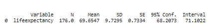
fig1, ax1 = plt.subplots() df_new = [df[df['Income_category']=='A']['lifeexpectancy'], df[df['Income_category']=='B']['lifeexpectancy'], df[df['Income_category']=='C']['lifeexpectancy'], df[df['Income_category']=='D']['lifeexpectancy'], df[df['Income_category']=='E']['lifeexpectancy']] ax1.set_title('life expectancy') ax1.boxplot(df_new) plt.show()

results = smf.ols('lifeexpectancy ~ C(Income_category)', data=df).fit() print (results.summary())

print ("Tukey") mc1 = multi.MultiComparison(df['lifeexpectancy'], df['Income_category']) print (mc1) res1 = mc1.tukeyhsd() print (res1.summary())

print ('means for for life expectancy by Income') m1= df.groupby('Income_category').mean() print (m1)

print ('Results') print ('standard deviations for life expectancy by Income') sd1 = df.groupby('Income_category').std() print (sd1)

Conclusions – ANOVA Analysis

An ANOVA test is carried out, integrated by 176 rows, 171 will be used for the test. A filter is applied to eliminate some incorrect values, such as non-numeric, negative, etc., reducing the rows of the original data set.

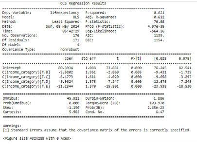
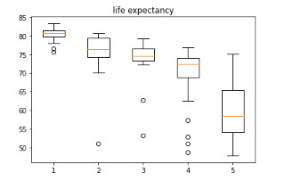
The ANOVA analysis shows a graph for each category (at the top) and, as can be seen, the life expectancy of class A, has a life expectancy of 80.39 years while the E class has a life expectancy of 59, 15 years

[detrasdeldataset]

Explorando la Relación entre Depresión, Consumo de Alcohol y Ocupación: Un Análisis de Varianza y Prueba F

¡Bienvenidos de nuevo a nuestro blog sobre el alcoholismo y la salud mental!

En esta ocasión, nos sumergiremos en el fascinante mundo del análisis de varianza (ANOVA) y la prueba F. Esta herramienta estadística nos permite explorar si existen diferencias significativas entre las medias de dos o más grupos. En nuestro estudio, nos enfocaremos en la variable "depresión" y en cómo se relaciona con el consumo total anual de alcohol.

La prueba F en este contexto se utiliza para determinar si hay una diferencia significativa entre las medias de dos grupos. En este caso, se estudiará la variable “depresión" la cual tiene dos niveles: True (presencia de depresión) y False (ausencia de depresión).

La hipótesis nula (H0) en la prueba F establece que no hay diferencia significativa entre las medias del consumo total anual para los dos grupos, es decir, que el consumo total anual es el mismo para las personas con y sin depresión.

Por otro lado, la hipótesis alternativa (H1) sugiere que hay al menos una diferencia significativa entre las medias de los grupos.

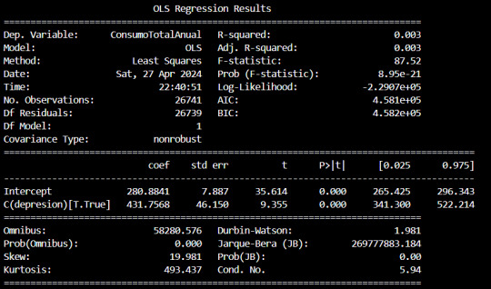
Dado que el valor p asociado con la prueba F es prácticamente cero (0.000), esto indica que hay suficiente evidencia para rechazar la hipótesis nula. Por lo tanto, concluimos que la media del consumo total anual de las personas difiere significativamente según si tienen depresión o no.

Durante la fase de visualización de datos, se observó que el porcentaje de alcoholismo variaba entre el 15% y el 17% para cada categoría ocupacional. Esta primera inspección sugirió inicialmente que podría no haber diferencias estadísticas significativas entre los grupos. Sin embargo, con el fin de verificar esta suposición de manera rigurosa, se optó por llevar a cabo un análisis de varianza (prueba F) para evaluar si existían diferencias estadísticamente significativas en la prevalencia de alcoholismo entre los distintos grupos ocupacionales. Los porcentajes que habíamos observado de alcoholismo por ocupación son:

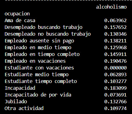
La prueba F se utilizó para determinar si existe una diferencia significativa entre las medias de la variable de respuesta (en este caso, el indicador de alcoholismo) entre los diferentes grupos definidos por la ocupación.

La hipótesis nula (H0) establece que no hay diferencia significativa entre las medias del indicador de alcoholismo para los diferentes grupos ocupacionales.

Mientras que la hipótesis alternativa (H1) sugiere que al menos una diferencia significativa está presente.

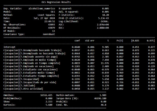
El resultado de la prueba F mostró un valor p de aproximadamente 5.13e-43, lo que indica que este valor es esencialmente cero. Por lo tanto, tenemos evidencia suficiente para rechazar la hipótesis nula y concluir que hay diferencias significativas en el indicador de alcoholismo entre los diferentes grupos ocupacionales.

Después de realizar la prueba F y rechazar la hipótesis nula, se llevaron a cabo comparaciones múltiples entre los diferentes grupos ocupacionales para determinar cuáles de ellos presentaban diferencias significativas en cuanto a la prevalencia de alcoholismo.

Las comparaciones múltiples se realizaron utilizando el método de Tukey HSD (Diferencia Significativa Mínima Honestamente). Este método ajusta el valor p para tener en cuenta el error de tipo I acumulado debido a las múltiples comparaciones.

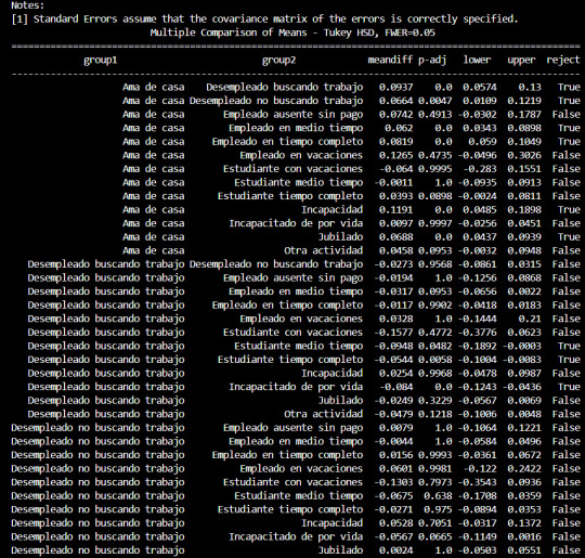
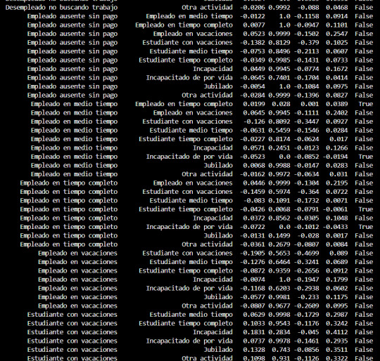
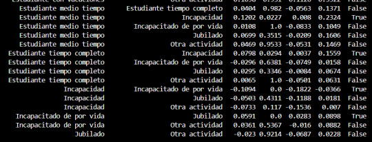
Los resultados de las comparaciones múltiples indicaron que hubo diferencias significativas en la prevalencia de alcoholismo entre varios pares de grupos ocupacionales. Se encontraron diferencias significativas entre ciertos grupos, mientras que otros no mostraron diferencias significativas.

Conclusión:

En conclusión, el análisis de varianza (ANOVA) y la prueba F nos han proporcionado una valiosa perspectiva sobre la relación entre la depresión, el consumo de alcohol y la ocupación. Hemos descubierto que las personas con depresión tienen un consumo total anual de alcohol significativamente diferente en comparación con aquellas sin depresión. Además, al analizar la prevalencia de alcoholismo entre diferentes grupos ocupacionales, encontramos diferencias significativas que nos brindan una comprensión más profunda de cómo el entorno laboral puede influir en los patrones de consumo de alcohol. Este análisis riguroso nos acerca un paso más a comprender los complejos vínculos entre el alcoholismo y la salud mental, lo que potencialmente podría informar estrategias más efectivas de prevención y tratamiento.

Puedes consultar el código y los datos con los que estamos trabajando aquí:

ANOVA.py

datos_nesarc.csv

[ebubekir-25]