#Error importing Seaborn module in Python

[ittrainingwithplacement]

What Tools and IDEs Are Used in a Typical Python Programming Training Course?

Introduction

Python is one of the most popular programming languages in the world, known for its simplicity and readability. It's used in web development, data science, AI, and more. But writing Python code effectively requires more than just understanding syntax; you need the right tools and integrated development environments (IDEs). In any comprehensive Python online training with certification, understanding and using these tools is a crucial part of the learning journey.

According to the 2024 Stack Overflow Developer Survey, Python ranks as the most wanted language among developers. This shows a strong industry demand and growing interest from beginners. To keep up, python programming online training courses are integrating a variety of tools and IDEs that help learners practice, debug, and build projects more efficiently.

In this blog, we’ll explore the most commonly used tools and IDEs in a typical Python programming training course. You’ll learn what each tool does, why it matters, and how it helps in real-world scenarios.

Understanding the Python Development Environment

Before diving into individual tools, it's important to understand what makes up a Python development environment. In a typical Python online training with certification, the environment includes:

An IDE or code editor for writing Python code.

A Python interpreter to run the code.

Package managers like pip to install libraries.

Version control tools to track project changes.

Notebooks or dashboards for interactive development. These components help create a seamless workflow for coding, testing, and debugging.

Top IDEs Used in Python Online Training With Certification

PyCharm

Why it’s used in Python courses: PyCharm by JetBrains is one of the most feature-rich IDEs for Python. It supports python language online development with intelligent code completion, error highlighting, and integrated debugging tools.

Features:

Integrated debugging and testing

Smart code navigation

Refactoring tools

Version control support

Integrated terminal and Python console

Example in training: In Python online training with certification, students often use PyCharm to work on object-oriented programming projects or web development with Django.

Visual Studio Code (VS Code)

Why it’s popular: VS Code is lightweight, open-source, and customizable. With the Python extension installed, it becomes a powerful tool for any Python programmer.

Features:

IntelliSense for Python

Built-in Git support

Extensive extensions marketplace

Integrated terminal

Jupyter Notebook support

Example in training: VS Code is commonly used when introducing learners to data science libraries like Pandas and NumPy.

Jupyter Notebook

Why it’s essential for data science: Jupyter is more than an IDE; it's a web-based interactive computing platform. It allows you to mix code, output, visualizations, and markdown.

Features:

Inline visualization (great for Matplotlib, Seaborn)

Segment-based execution

Easy documentation with Markdown

Works seamlessly with Anaconda

Example in training: Used extensively in Python online training with certification for data analysis, machine learning, and statistics-based modules.

IDLE (Integrated Development and Learning Environment)

Why it’s beginner-friendly: IDLE is Python’s built-in IDE. While basic, it’s often introduced first to help learners focus on understanding syntax and logic without distractions.

Features:

Lightweight and easy to install

Simple REPL environment

Good for small scripts and exercises

Example in training: Used during the early phase of the course for learning variables, control flow, and functions.

Essential Tools for Python Programming

Python Interpreter

Every Python course requires a Python interpreter to execute the code. Python 3.x is the standard for most training programs today.

Key Use: Interprets and executes your code line-by-line, providing immediate output or error messages.

Anaconda Distribution

Why it’s useful: Anaconda is a bundle that includes Python, Jupyter, and hundreds of scientific libraries. It's widely used in data-heavy training modules.

Benefits:

Easy package management via Conda

Comes with Jupyter pre-installed

Ideal for machine learning and data analysis

Real-world tie-in: Many professionals use Anaconda in industry settings for AI and analytics work, making it highly relevant in Python online training with certification.

Version Control and Collaboration Tools

Git and GitHub

Why it's taught in courses: Version control is a must-have skill. Students are introduced to Git for local version tracking and GitHub for remote collaboration.

How it’s used:

Commit and push changes

Work in teams on group assignments

Review and merge pull requests

Example Project: Building a multi-file Python project with collaboration using Git branches.

Python Package Management Tools

pip (Python Package Installer)

Used in nearly every course, pip allows students to install packages from the Python Package Index (PyPI).

Command Example:

bash

pip install requests

virtualenv and venv

These tools are used to create isolated environments, avoiding package conflicts across projects.

Why it matters in training: It teaches learners how to manage dependencies correctly.

Code Linters and Formatters

Pylint and Flake8

These tools help identify syntax errors, poor coding practices, and PEP8 violations.

How it helps learners:

Immediate feedback on bad code

Encourages good coding habits

Prepares for real-world collaboration

Black

Black is an automatic code formatter that enforces a uniform style.

Why it’s taught: In professional development environments, consistent code style is crucial. Black makes that easy.

Jupyter Notebooks and Interactive Coding Tools

Google Colab

Why it’s included: Google Colab provides free cloud-based Jupyter notebooks with GPU support. It’s great for training AI and ML models.

Features:

No local setup required

Supports Python 3 and major libraries

Shareable and collaborative

Thonny

A beginner-friendly IDE ideal for introducing students to debugging and variable tracking visually.

Used for: Explaining loops, conditionals, and function scopes visually.

Real-World Applications in Training Projects

Web Development

Tools Used: PyCharm, Flask/Django, GitHub

Project Example: Build a blog website with CRUD features.

Data Analysis

Tools Used: Jupyter, Pandas, Matplotlib

Project Example: Analyze COVID-19 datasets and visualize trends.

Machine Learning

Tools Used: Google Colab, Scikit-learn, TensorFlow

Project Example: Build a linear regression model to predict housing prices.

Automation Scripts

Tools Used: VS Code, Selenium

Project Example: Automate login and data scraping from websites.

Key Takeaways

Python online training with certification includes tools that mirror real-world job roles.

IDEs like PyCharm and VS Code enhance learning through code suggestions, debugging, and integration.

Jupyter and Colab are essential for data-driven modules.

Git, pip, and virtual environments introduce real-world development workflows.

Code linters and formatters help build professional-level coding habits.

Conclusion

Whether you're aiming for data science, web development, or automation, understanding the tools and IDEs used in a python programming training course is crucial. These tools don't just make learning easier, they prepare you for real-world coding jobs.

Ready to sharpen your Python skills and build job-ready projects? Start learning with the right tools today!

[shalu620]

How Much Python Do You Need to Know to Secure a Job?

If you're looking to break into a career that uses Python, you might wonder just how much you need to learn. The depth of knowledge required varies depending on the job role you are targeting. Here's a detailed guide on the essential skills and knowledge you should acquire to enhance your job prospects. Considering the kind support of Learn Python Course in Pune, Whatever your level of experience or reason for switching from another programming language, learning Python gets much more fun.

Foundational Knowledge

Starting with the basics is crucial. Here are the key areas to focus on initially:

Python Syntax and Basics

Grasping the basic syntax and core concepts of Python is essential. This includes understanding:

Variables and Data Types: How to define and use different types like integers, floats, strings, and booleans.

Operators: Using arithmetic, logical, and comparison operators.

Control Structures: Implementing loops (for, while) and conditionals (if, elif, else).

Functions and Modules

Knowing how to write and use functions will make your code more organized and reusable. You should:

Define Functions: Understand parameters, return values, and scope.

Work with Modules: Learn to import and utilize various Python modules.

Data Structures

Get acquainted with Python’s built-in data structures:

Lists: Ordered and mutable collections.

Dictionaries: Key-value pairs.

Tuples: Immutable collections.

Sets: Unordered collections of unique elements. Enrolling in the Best Python Certification Online can help people realise Python’s full potential and gain a deeper understanding of its complexities.

Intermediate Proficiency

Once you’re comfortable with the basics, move on to more advanced topics:

Object-Oriented Programming (OOP)

OOP is a powerful feature of Python essential for many applications. Learn about:

Classes and Objects: Creating and using classes and instances.

Inheritance: Extending classes and reusing code.

Polymorphism: Methods that can operate on objects of different classes.

Exception Handling

Building robust programs requires handling errors gracefully. You should:

Use Try-Except Blocks: Manage exceptions without crashing your program.

Debugging: Learn techniques and tools to troubleshoot and fix issues.

File Input/Output

Interacting with files is a common requirement. Know how to:

Read and Write Files: Open, read, write, and close files using Python.

Libraries and Frameworks

Familiarize yourself with essential libraries to enhance your productivity:

NumPy: For numerical computations.

Pandas: For data manipulation and analysis.

Requests: For making HTTP requests.

Advanced Skills and Specializations

Depending on your career path, you might need to dive deeper into specific areas:

Web Development

For web development roles, mastering web frameworks is crucial:

Django: A comprehensive framework for building robust web applications.

Flask: A lightweight framework suitable for smaller applications and microservices.

Data Science and Machine Learning

If you're leaning towards data-centric roles, focus on:

Machine Learning Libraries: TensorFlow and PyTorch for building models.

Data Analysis Tools: Scikit-Learn for machine learning algorithms, Matplotlib, and Seaborn for data visualization.

Automation and Scripting

Automating tasks can greatly improve efficiency. Learn to:

Write Scripts: Automate repetitive tasks.

Web Scraping: Use BeautifulSoup or Scrapy to extract data from websites.

APIs: Interact with web services to send and receive data.

Gaining Practical Experience

Theory is important, but hands-on experience is invaluable:

Real-World Projects

Work on projects that solve real problems. This will deepen your understanding and provide you with a portfolio to show potential employers.

Coding Challenges

Participate in coding challenges on platforms like:

LeetCode

HackerRank

CodeSignal

These challenges sharpen your problem-solving skills and prepare you for technical interviews.

Version Control with Git

Learn to use Git for version control. Understanding commits, branches, merges, and pull requests is crucial for collaborating on projects. Host your code on platforms like GitHub or GitLab to showcase your work.

Essential Soft Skills

Technical abilities alone aren’t enough. Employers also value:

Problem-Solving Skills

Show that you can approach and solve problems logically and efficiently. Strong problem-solving skills are crucial for tackling challenges and developing innovative solutions.

Communication Skills

Being able to explain your code and thought process clearly, both verbally and in writing, is essential. Good communication skills are important for collaborating with team members and presenting your ideas effectively.

Navigating the Job Market

Building a Resume and Portfolio

Create a resume that highlights your Python skills and experience. Tailor it to the jobs you're applying for and include links to your GitHub profile or personal website to showcase your projects.

Networking

Join Python communities, attend meetups, and connect with professionals on LinkedIn. Networking can provide job opportunities, industry insights, and professional connections that can help you advance in your career.

Conclusion

Mastering every aspect of Python isn't necessary to land a job, but having a solid understanding of the basics and building upon that foundation is key. Specialize based on the job you're targeting, and gain practical experience through projects and coding challenges. Continuous learning and improvement will significantly boost your job prospects. Focus on developing both your technical and soft skills, and actively engage in the job search process to maximize your chances of success.

[techhelpnotes]

Error importing Seaborn module in Python

I had faced the same problem. Restarting the notebook solved my problem.

If that doesnt solve the problem, you can try this

As @avp says the bash line pip install seaborn should work I just had the same problem and and restarting the notebook didnt seem to work but running the command as jupyter line magic was a neat way to fix the problem without restarting the notebook

[poudelbibek]

Data visualization Module 4 Assignment

Data visualization Assignment 4

Reminder (research problem and defined variables)

Study topic:

Primary topic

Suicide rate Vs. various socio-economic reasons (income per person/ employment rate/ country’s political score)

Variables of interest:

Python program

#importing libraries

import pandas

import numpy as np

import matplotlib.pyplot as plt

import seaborn

#Reading data

data = pandas.read_csv('gapminder_data.csv', low_memory=False)

#setting variables of interest to numeric

data['suicideper100th'] = pandas.to_numeric(data['suicideper100th'],errors = 'coerce')

data['employrate'] = pandas.to_numeric(data['employrate'],errors = 'coerce')

data['polityscore'] = pandas.to_numeric(data['polityscore'],errors = 'coerce')

data['incomeperperson'] = pandas.to_numeric(data['incomeperperson'],errors = 'coerce')

#Coding out missing data or Filtering countries with valid data for various variables

#Filtering countries with valid suicidedata and determine center and spread

suicidedata = data[data['suicideper100th'].notna()]  

Num_suicidedata = len(suicidedata)

print('Number of countries with available suicide data:', Num_suicidedata)

print('Number of countries with missing suiciderate data:', len(data)-Num_suicidedata)

suicidedata['suicideper100th'].describe()

Output

Number of countries with available suicide data: 191

Number of countries with missing suiciderate data: 22

count    191.000000

mean       9.640839

std        6.300178

min        0.201449

25%        4.988449

50%        8.262893

75%       12.328551

max       35.752872

Name: suicideper100th, dtype: float64

Discussion:

Range: 0.2-35.75

Center (Mean): 9.64

Center (Median): 8.26

Standard deviation: 6.3

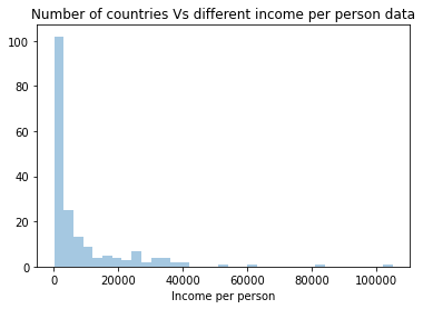
#Filtering countries with valid income data

incomedata = data[data['incomeperperson'].notna()]      

Num_incomedata = len(incomedata)

print('Number of countries with available incomeperperson data:', Num_incomedata)

print('Number of countries with missing incomeperperson data:', len(data)-Num_incomedata)

incomedata['incomeperperson'].describe()

Output:

Number of countries with available incomeperperson data: 190

Number of countries with missing incomeperperson data: 23

Out[45]:

count       190.000000

mean       8740.966076

std       14262.809083

min         103.775857

25%         748.245151

50%        2553.496056

75%        9379.891166

max      105147.437700

Name: incomeperperson, dtype: float64

Discussion:

Range: 103.77 – 105147.43

Center (Mean): 8740.96

Center (Median): 2553.49

Standard deviation: 14262.80

#Filtering countries with valid employment rate data

employratedata = data[data['employrate'].notna()]     

Num_employratedata = len(employratedata)

print('Number of countries with available employment rate data:', Num_employratedata)

print('Number of countries with missing employment rate data:', len(data)-Num_employratedata)

employratedata['employrate'].describe()

Output

Number of countries with available employment rate data: 178

Number of countries with missing employment rate data: 35

Out[44]:

count    178.000000

mean      58.635955

std       10.519454

min       32.000000

25%       51.225000

50%       58.699999

75%       64.975000

max       83.199997

Name: employrate, dtype: float64

Discussion:

Range: 32-83.19

Center (Mean): 58.63

Center (Median): 58.69

Standard deviation: 10.52

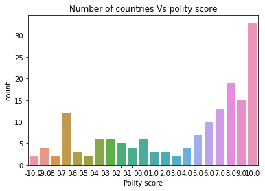
#Filtering countries with valid political score data

politydata = data[data['polityscore'].notna()]     

Num_politydata = len(politydata)

print('Number of countries with available political score data:', Num_politydata)

print('Number of countries with missing political score data:', len(data)-Num_politydata)

politydata['polityscore'].describe()

Output

Number of countries with available political score data: 161

Number of countries with missing political score data: 52

Out[22]:

count    161.000000

mean       3.689441

std        6.314899

min      -10.000000

25%       -2.000000

50%        6.000000

75%        9.000000

max       10.000000

Name: polityscore, dtype: float64

Discussion:

Range: -10 to 10

Center (Mean): 3.68

Center (Median): 6

Standard deviation: 6.31

#Univariate histogram for suicide data:

seaborn.distplot(suicidedata['suicideper100th'].dropna(), kde=False);

plt.xlabel('Number of suicide per 100000')

plt.title('Number of countries Vs suicide per 100000 according to gapminder data')

#Univariate histogram for income data:

seaborn.distplot(incomedata['incomeperperson'].dropna(), kde=False);

plt.xlabel('Income per person')

plt.title('Number of countries Vs different income per person data')

#Univariate histogram for employment rate data:

seaborn.distplot(employratedata['employrate'].dropna(), kde=False);

plt.xlabel('Employment rate')

plt.title('Number of countries Vs different employment rate data')

#Univariate histogram for political score data:

politydata['polityscore']= politydata['polityscore'].astype('category')

seaborn.countplot(x="polityscore", data=politydata);

plt.xlabel('Polity score')

plt.title('Number of countries Vs polity score')

#Plotting histograms of each variable

#Alternative way to generate histogram

plt.figure(figsize=(16,12))

plt.subplot(2,2,1)

plt.title('Suicide rate or suicideper100th')

suicidedata['suicideper100th'].hist(bins=10)

plt.subplot(2,2,2)

incomedata['incomeperperson'].hist(bins=10)

plt.title('Income per person')

plt.subplot(2,2,3)

employratedata['employrate'].hist(bins=10)

plt.title('Employment rate')

plt.subplot(2,2,4)

politydata['polityscore'].hist(bins=10)

plt.title('Political score or polityscore')

Discussion from univariate plots

It is quite clear from the univariate histogram plots that the number of suicide and income per person data is skewed left, employment rate data is unimodal and almost-normally distributed whereas the political score is skewed right. This means that the most of the countries have lower suicide rate and lower income data and only few countries have exceptionally high number for both these data. Employment rate is near-normal distribution meaning the data are spread uniformly about the mean center of the employment rate. Political score of most countries are more than the mean (which is zero). Hence, more countries have positive political score and there are lesser number of countries with negative political score.

#Binning and creating new category

#Categorizing countries in 5 different levels

bins = [0,1000,5000,10000,25000,300000]

group_names = ['Very poor,0-1000', 'Poor,1000-5000', 'Medium,5000-10000', 'Rich,10000-25000','Very rich,25000-300000']

categories = pandas.cut(incomedata['incomeperperson'], bins, labels=group_names)

incomedata['categories']= pandas.cut(incomedata['incomeperperson'], bins, labels=group_names)

pandas.value_counts(categories)

Output

Poor,1000-5000            61

Very poor,0-1000          54

Medium,5000-10000         28

Very rich,25000-300000    24

Rich,10000-25000          23

Name: incomeperperson, dtype: int64

#Bivariate plots

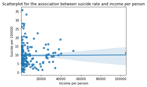
scat1 = seaborn.regplot(x="incomeperperson", y="suicideper100th", fit_reg=True, data=suicidedata)

plt.xlabel('Income per person')

plt.ylabel('Suicide per 100000')

plt.title('Scatterplot for the association between suicide rate and income per person')

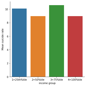
# quartile split (use qcut function & ask for 4 groups - gives you quartile split)

print ('Income per person - 4 categories - quartiles')

incomedata['INCOMEGRP4']=pandas.qcut(incomedata.incomeperperson, 4, labels=["1=25th%tile","2=50%tile","3=75%tile","4=100%tile"])

c10 = incomedata['INCOMEGRP4'].value_counts(sort=False, dropna=True)

print(c10)

# bivariate bar graph C->Q

seaborn.catplot(x='INCOMEGRP4', y='suicideper100th', data=incomedata, kind="bar", ci=None)

plt.xlabel('income group')

plt.ylabel('Mean suicide rate')

c11= incomedata.groupby('INCOMEGRP4').size()

print (c11)

Output

Income per person - 4 categories - quartiles

1=25th%tile    48

2=50%tile      47

3=75%tile      47

4=100%tile     48

Name: INCOMEGRP4, dtype: int64

INCOMEGRP4

1=25th%tile    48

2=50%tile      47

3=75%tile      47

4=100%tile     48

dtype: int64

#Bivariate plot for suicide rate vs employment rate

scat2 = seaborn.regplot(x="employrate", y="suicideper100th", fit_reg=True, data=suicidedata)

plt.xlabel('Employment rate')

plt.ylabel('Suicide per 100000')

plt.title('Scatterplot for the association between suicide rate and employment rate')

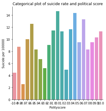
#Bivariate C->Q plot for suicide rate vs political score

suicidedata["polityscore"] = suicidedata["polityscore"].astype('category')

seaborn.catplot(x="polityscore", y="suicideper100th", data=suicidedata, kind="bar", ci=None)

plt.xlabel('Polityscore')

plt.ylabel('Suicide per 100000')

plt.title('Categorical plot of suicide rate and political score')

# quartile split (use qcut function & ask for 4 groups - gives you quartile split)

politydata['polityscore4']=pandas.qcut(politydata.polityscore, 4, labels=["1=25th%tile","2=50%tile","3=75%tile","4=100%tile"])

c12 = politydata['polityscore4'].value_counts(sort=False, dropna=True)

print(c12)

# bivariate bar graph C->Q

seaborn.catplot(x='polityscore4', y='suicideper100th', data=politydata, kind="bar", ci=None)

plt.xlabel('political score grp')

plt.ylabel('Mean suicide rate')

c13= politydata.groupby('polityscore').size()

print (c13)

Output

1=25th%tile    42

2=50%tile      39

3=75%tile      47

4=100%tile     33

Name: polityscore4, dtype: int64

polityscore

-10.0     2

-9.0      4

-8.0      2

-7.0     12

-6.0      3

-5.0      2

-4.0      6

-3.0      6

-2.0      5

-1.0      4

 0.0      6

 1.0      3

 2.0      3

 3.0      2

 4.0      4

 5.0      7

 6.0     10

 7.0     13

 8.0     19

 9.0     15

 10.0    33

dtype: int64

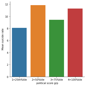
Discussion from bivariate plots

It is clear from the scatter plot that the income per person have almost no relationship with the suicide data. There is neither positive nor negative slope (the line seems to be almost horizontal). It is further confirmed by categorical bar chart as well. When income data was split into 4 categories, the mean suicide rate still didn’t show the clear trend. All the income categories had almost same mean suicide rate. Similar trend was seen for employment rate and political score as well.

[andidatachief56]

data analysis tools week 3

Hello,

following correlation is to be calculated:   Is there a correlation between the Age und the quantity of beer consuming each day.

Dataset: nesarc_pds.csv

2 quantative Variables choosen: 342-343 S2AQ5D NUMBER OF BEERS USUALLY CONSUMED ON DAYS WHEN DRANK BEER IN LAST 12 MONTHS 18268 1-42. Number of beers    78 99. Unknown    24747 BL. NA did not drink or unknwon

68-69 AGE     AGE       43079 18-97. Age in years      14 98. 98 years or older

Program: A sub- dataframe was created with the 2 choosen variables 'AGE' and 'S2AQ5D'. All unknown and NA rows dropped as well as all drinker of only 1 beer to remove the ground noise. By using the Pearsson- correlation function of the stats- module the correlation between both variables are calculated

Result:   The r- value = -0,15, that means almost no correlation between the Age and the quantity of beer each day.  

------------------------------------------------------------------------------------------------------- Program:

import os import pandas import numpy import seaborn import scipy.stats

# define individual name of dataset data = pandas.read_csv('nesarc_pds.csv', low_memory=False)

# recode missing values to python missing (NaN) data['S2AQ5D']=data['S2AQ5D'].replace('99', numpy.nan)    # defined as char data['S2AQ5D']=data['S2AQ5D'].replace(' ', numpy.nan)    # needed before set to numeric

# new code setting variables you will be working with to numeric data['S2AQ5D'] = pandas.to_numeric(data['S2AQ5D'], errors='coerce')

# data subset only for needed columns sub1 = data[['AGE','S2AQ5D']]

#make a copy of my new subsetted data   !! wichtig !!!   Remove NaN sub2 = sub1.copy()

print(len(sub2))              # No. of rows print(len(sub2.columns))  

sub2 = sub2.dropna()

print(' ---  nach dropNA ----') print(len(sub2))              # No. of rows print(len(sub2.columns))   print(sub2.value_counts(subset='S2AQ5D', normalize=True))    # in Prozent

sub2=sub2[(sub2['S2AQ5D']>1)]      # drop all rows with 1 beer

print(' ---  nach remove 1-3 ----') print(len(sub2))              # No. of rows print(len(sub2.columns))   print(sub2.value_counts(subset='S2AQ5D', normalize=True))    # in Prozent

scat1 = seaborn.regplot(x="AGE", y="S2AQ5D", fit_reg=True, data=sub2) plt.xlabel('AGE') plt.ylabel('Drinking beer per day') plt.title('Scatterplot for the Association Between AGE and consuming beer')

print ('association between AGE and consuming beer') print (scipy.stats.pearsonr(sub2['AGE'], sub2['S2AQ5D']))

---------------------------------------------------------------------------------------------

association between AGE and consuming beer (-0.15448800873680543, 1.7107443117251883e-60)

[webscreenscraping]

How To Scrape Stock Market Data Using Python?

The coronavirus pandemic has proved that the stock market is also volatile like all other business industries as it may crash within seconds and may also skyrocket in no time! Stocks are inexpensive at present because of this crisis and many people are involved in getting stock market data for helping with the informed options.

Unlike normal web scraping, extracting stock market data is much more particular and useful to people, who are interested in stock market investments.

Web Scraping Described

Web scraping includes scraping the maximum data possible from the preset indexes of the targeted websites and other resources. Companies use web scraping for making decisions and planning tactics as it provides viable and accurate data on the topics.

It's normal to know web scraping is mainly associated with marketing and commercial companies, however, they are not the only ones, which benefit from this procedure as everybody stands to benefit from extracting stock market information. Investors stand to take benefits as data advantages them in these ways:

Investment Possibilities

Pricing Changes

Pricing Predictions

Real-Time Data

Stock Markets Trends

Using web scraping for others’ data, stock market data scraping isn’t the coolest job to do but yields important results if done correctly. Investors might be given insights on different parameters, which would be applicable for making the finest and coolest decisions.

Scraping Stock Market and Yahoo Finance Data with Python

Initially, you’ll require installing Python 3 for Mac, Linux, and Windows. After that, install the given packages to allow downloading and parsing HTML data: and pip for the package installation, a Python request package to send requests and download HTML content of the targeted page as well as Python LXML for parsing with the Xpaths.

Python 3 Code for Scraping Data from Yahoo Finance

from lxml import html import requests import json import argparse from collections import OrderedDict def get_headers(): \ return {"accept": "text/html,application/xhtml+xml,application/xml;q=0.9,image/webp,image/apng,*/*;q=0.8,application/signed-exchange;v=b3;q=0.9", \ "accept-encoding": "gzip, deflate, br", \ "accept-language": "en-GB,en;q=0.9,en-US;q=0.8,ml;q=0.7", \ "cache-control": "max-age=0", \ "dnt": "1", \ "sec-fetch-dest": "document", \ "sec-fetch-mode": "navigate", \ "sec-fetch-site": "none", \ "sec-fetch-user": "?1", \ "upgrade-insecure-requests": "1", \ "user-agent": "Mozilla/5.0 (Windows NT 10.0; Win64; x64) AppleWebKit/537.36 (KHTML, like Gecko) Chrome/81.0.4044.122 Safari/537.36"} def parse(ticker): \ url = "http://finance.yahoo.com/quote/%s?p=%s" % (ticker, ticker) \ response = requests.get( \ url, verify=False, headers=get_headers(), timeout=30) \ print("Parsing %s" % (url)) \ parser = html.fromstring(response.text) \ summary_table = parser.xpath( \ '//div[contains(@data-test,"summary-table")]//tr') \ summary_data = OrderedDict() \ other_details_json_link = "https://query2.finance.yahoo.com/v10/finance/quoteSummary/{0}?formatted=true&lang=en-US®ion=US&modules=summaryProfile%2CfinancialData%2CrecommendationTrend%2CupgradeDowngradeHistory%2Cearnings%2CdefaultKeyStatistics%2CcalendarEvents&corsDomain=finance.yahoo.com".format( \ ticker) \ summary_json_response = requests.get(other_details_json_link) \ try: \ json_loaded_summary = json.loads(summary_json_response.text) \ summary = json_loaded_summary["quoteSummary"]["result"][0] \ y_Target_Est = summary["financialData"]["targetMeanPrice"]['raw'] \ earnings_list = summary["calendarEvents"]['earnings'] \ eps = summary["defaultKeyStatistics"]["trailingEps"]['raw'] \ datelist = [] \ for i in earnings_list['earningsDate']: \ datelist.append(i['fmt']) \ earnings_date = ' to '.join(datelist) \ for table_data in summary_table: \ raw_table_key = table_data.xpath( \ './/td[1]//text()') \ raw_table_value = table_data.xpath( \ './/td[2]//text()') \ table_key = ''.join(raw_table_key).strip() \ table_value = ''.join(raw_table_value).strip() \ summary_data.update({table_key: table_value}) \ summary_data.update({'1y Target Est': y_Target_Est, 'EPS (TTM)': eps, \ 'Earnings Date': earnings_date, 'ticker': ticker, \ 'url': url}) \ return summary_data \ except ValueError: \ print("Failed to parse json response") \ return {"error": "Failed to parse json response"} \ except: \ return {"error": "Unhandled Error"} if __name__ == "__main__": \ argparser = argparse.ArgumentParser() \ argparser.add_argument('ticker', help='') \ args = argparser.parse_args() \ ticker = args.ticker \ print("Fetching data for %s" % (ticker)) \ scraped_data = parse(ticker) \ print("Writing data to output file") \ with open('%s-summary.json' % (ticker), 'w') as fp: \ json.dump(scraped_data, fp, indent=4)

Real-Time Data Scraping

As the stock market has continuous ups and downs, the best option is to utilize a web scraper, which scrapes data in real-time. All the procedures of data scraping might be performed in real-time using a real-time data scraper so that whatever data you would get is viable then, permitting the best as well as most precise decisions to be done.

Real-time data scrapers are more costly than slower ones however are the finest options for businesses and investment firms, which rely on precise data in the market as impulsive as stocks.

Advantages of Stock Market Data Scraping

All the businesses can take advantage of web scraping in one form particularly for data like user data, economic trends, and the stock market. Before the investment companies go into investment in any particular stocks, they use data scraping tools as well as analyze the scraped data for guiding their decisions.

Investments in the stock market are not considered safe as it is extremely volatile and expected to change. All these volatile variables associated with stock investments play an important role in the values of stocks as well as stock investment is considered safe to the extent while all the volatile variables have been examined and studied.

To collect as maximum data as might be required, you require to do stock markets data scraping. It implies that maximum data might need to be collected from stock markets using stock market data scraping bots.

This software will initially collect the information, which is important for your cause as well as parses that to get studied as well as analyzed for smarter decision making.

Studying Stock Market with Python

Jupyter notebook might be utilized in a course of the tutorial as well as you can have it on GitHub.

Setup Procedure

You will start installing jupyter notebooks because you have installed Anaconda

Along with anaconda, install different Python packages including beautifulsoup4, fastnumbers, and dill.

Add these imports to the Python 3 jupyter notebooks

import numpy as np # linear algebra import pandas as pd # pandas for dataframe based data processing and CSV file I/O import requests # for http requests from bs4 import BeautifulSoup # for html parsing and scraping import bs4 from fastnumbers import isfloat from fastnumbers import fast_float from multiprocessing.dummy import Pool as ThreadPool import matplotlib.pyplot as plt import seaborn as sns import json from tidylib import tidy_document # for tidying incorrect html sns.set_style('whitegrid') %matplotlib inline from IPython.core.interactiveshell import InteractiveShell InteractiveShell.ast_node_interactivity = "all"

What Will You Require Extract the Necessary Data?

Remove all the excessive spaces between the strings

A few strings from the web pages are available with different spaces between words. You may remove it with following:

def remove_multiple_spaces(string): \ if type(string)==str: \ return ' '.join(string.split()) \ return string

Conversions of Strings that Float

In different web pages, you may get symbols mixed together with numbers. You could either remove symbols before conversions, or you utiize the following functions:

def ffloat_list(string_list): \ return list(map(ffloat,string_list))

Sending HTTP Requests using Python

Before making any HTTP requests, you require to get a URL of a targeted website. Make requests using requests.get, utilize response.status_code for getting HTTP status, as well as utilize response.content for getting a page content.

Scrape and Parse the JSON Content from the Page

Scrape json content from the page with response.json() and double check using response.status_code.

Scraping and Parsing HTML Data

For that, we would use beautifulsoup4 parsing libraries.

Utilize Jupyter Notebook for rendering HTML Strings

Utilize the following functions:

from IPython.core.display import HTML HTML("Rendered HTML")

Find the Content Positions with Chrome Inspector

You’ll initially require to know HTML locations of content that you wish to scrape before proceeding. Inspect a page with Mac or chrome inspector using the functions cmd+option+I as well as inspect for the Linux using a function called Control+Shift+I.

Parse a Content and Show it using BeautifulSoup4

Parse a content with a function BeautifulSoup as well as get content from the header 1 tag as well as render it.

A web scraper tool is important for investment companies and businesses, which need to buy stocks as well as make investments in stock markets. That is because viable and accurate data is required to make the finest decisions as well as they could only be acquired by scraping and analyzing the stock markets data.

There are many limitations to extracting these data however, you would have more chances of success in case you utilize a particularly designed tool for the company. You would also have a superior chance in case, you use the finest IPs like dedicated IP addresses provided by Web Screen Scraping.

For more information, contact Web Screen Scraping!

[365daysofquant]

#5 Statistical arbitrage

Date: 27 July 2021

Firstly, I need to understand what exactly statistical arbitrage means, and then we can write up a small aim of the project and code it out on a notebook and hopefully push it to GitHub as well.

Statistical arbitrage are trading strategies that take advantage of mean reversing in stock prices or opportunities created in market anomalies. the blog I'm following uses pairs trading so I’ll use it too. 

Pairs trading is when you take two stocks that are cointegrated (I'm guessing this means that the correlation coefficient is positive). When there is a deviation in the price of these two stocks, we expect the price to come back to a mean point (”mean reverting”) and we can make a benefit on the trade here by buying the underperforming one (since it’ll rise up) and short the over performing one (since it’ll drop). but if the price divergence is not temporary (i.e structural) you can lose the money.

The blog itself uses NSE100 to pick 15 stocks and it seems they had the closing price for these in a csv file already. I’ll try to import the data using yahoo tickers and put it in a data frame, which means I need to stock pick first. Lets use google search to find top 25 US stocks? might be difficult to find arbitrage with US markets tho. But data will be easier to find. Okay let’s try US first.

I got the tickers of the top 25 stocks on the S&P 500. Turns out the Berkshire Hathaway Inc. Class B ticker gave some Date error (weird) so I'm just gonna leave that out. Currently I'm also struggling with getting non stock data onto python, which is something I should figure out for CSIC since the largest chunk of the score is given to diversification. I’ll make a separate post on CSIC later actually so we can get a hang of that too.

Back to this. Imported my data by the same method as the optimiser bot. removed the na values too.

we now split the data into test and train data. this is to ensure that the decision to select the cointegrated pair is done from the training dataset and the backtesting is done on the test dataset.

to do this I import the train_test_split module from sklearn which is the machine learning library on python. I chose to split with a 50-50 % ratio, so test_size = 0.5

To understand the correlation between the stocks, we use Pearson correlation coefficient. The function ‘coint’ from statsmodels will return the p-value of a cointegration test. The null hypothesis is that cointegration is zero. So if the p-value is < 0.05, we can reject the null and assume a cointegrated pair. 

First things first, we get the correlation matrix. I make a figure using plt.subplots(figsize=(x,y)) to make a ‘figure’ and then use seaborn, another data analytics library to make the correlation matrix. 

import seaborn as sns

sns.heatmap(train.pct_change().corr(method = 'pearson'), ax = ax, cmap = 'coolwarm', annot=True, fmt =".2f") ax.set_title('Asset Correlation Matrix')

The pct_change() function converts the closing price to returns, the .corr gives the correlation. cannot = True gives a data value in each cell. I'm guessing fmt rounds off the correlation coefficient, so in our case .2f indicates round off to 2 places.

we now code a function to identify the cointegrated pairs.

the function looks complicated but the idea is very basic. We first iterate through all the data (i) and then iterate through the data in front of I (j which goes from i+1 to n), and run the ‘coint’ function on the pair (i, j). 

If we check the documentation, we get three outputs from coint:

1. coint_t: the t-statistic for the test

2. pvalue of the test

and 3. crit_value: or the critical value of the test at 1%, 5% and 10% significance levels. This is just basic hypothesis testing results.

since we want the p-value, we take store coint in result, and chose to store in the p-value matrix, the value of result[1]. 

If this p-value is less than 0.05, we reject the null and so we code exactly that: 

if result[1] < 0.05: 

we store the pair data[I] and data[j] into a new list pairs. This list is the complete “list” of cointegrated pairs from all the stocks we have.

Let’s finish the rest next time!

[engrflores]

Regression Modeling in Practice

Regression Modeling in Practice - Week 4 ( Test a Logistic Regression Model )

On this blog, I will test the association between my binary response variable, major depression which is coded 0 = No, 1 = Yes and my binary explanatory variable Personal income which I bin out into two categories which is 0 = Low income(<= $23000), 1 = High income (<= $100000) with 13705 young adults (Age 18-35) as my sample. Using logistics regression as my multivariate tool to test the association between two binary categorical variables, here are the results:

LOGISTIC REGRESSION

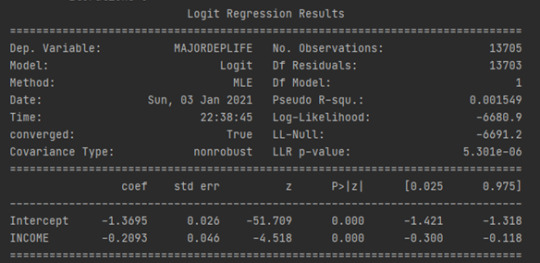
Notice also that our regression is significant at a P value of less than 0.05. Using the prime assessments, we could generate the linear equation. Major depression is a function of 0.026 plus 0.046 times Income but let's really think about the equation some more.

In a regression module, our response variable was quantitative. And so, it could theoretically take on any value. In a logistic regression, our response variable only takes on the values zero and one. Therefore, if I try to use this equation as a best fit line, I would run into some problems.

Instead of talking in decimals it may be more helpful for us to talk about how the probability of being Major depression changes based on the Income level. Instead of true expected values, we want probabilities using our logistics regression model through Odds ratios:

By definition: The odds ratio is the probability of an event occurring in one group compared to the probability of an event occurring in another group. Odds ratios are always given in the form of odds and are not linear. The odds ratio is the natural exponentiation of our parameter estimate. Thus, all that we need to do is calculate the natural log to the power of our parameter estimate. Here are my results:

ODDS RATIOS

Here are the results. Because both my explanatory and response variables in the model are binary, coded zero and one. I can interpret the odds ratio in the following way. Since it was less than 1 which is 0.81, High income young adults in my sample are 0.81 times less likely to have major depression than low income young adult.

CONFIDENCE INTERVALS

Looking at the confidence interval, we can get a better picture of how much this value would change for a different sample drawn from the population. Based on our model, high income young adults are anywhere from 0.74 to 0.89 times less likely to have major depression than those low income young adults. The odds ratio is a sample statistic and the confidence intervals are an estimate of the population parameter.

 Now, I want to test a potential confounder to add in my model which is Gender. I’ve run another logistic regression with Gender as my potential confounder and here are the results:

LOGISTIC REGRESSION

As we can see, both Personal Income and Gender are independently associated with the likelihood of having major depression but they are negatively associated with a likelihood of having major depression. Gender is not a confounder between my Primary response variable and Primary explanatory variable.

ODDS RATIOS

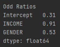
In our predictor or splinter variables are both binary, we can interpret the odds ratio in the following way. High income young adults in my sample are 0.91 times less likely to have major depression than low income young adult after controlling for major depression. Also, Male young adults in my sample are 0.53 times less likely to have major depression than Female young adult after controlling for major depression.

 CONFIDENCE INTERVALS:

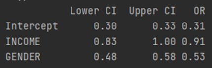
Because the confidence intervals on our odds ratios overlap, we cannot say that Personal income is more strongly associated with Major depression than Gender. For the population of High income young adults, we can say that those high income young adults are anywhere between 0.83 to 1 times less likely to have major depression than low income young adult. And those Male young adults are between 0.48 and 0.58 times less likely to have major depression than Female young adults. Both of these estimates are calculated after accounting for the alternate disorder. As with multiple regression, when using logistic regression, we can continue to add variables to our model in order to evaluate multiple predictors of our binary categorical response variable. Presence or absence of major depression.

My Python Code:

import numpy as np import pandas as pd import statsmodels.api as sm import seaborn import statsmodels.formula.api as smf import matplotlib.pyplot as plt # bug fix for display formats to avoid run time errors pd.set_option('display.float_format', lambda x:'%.2f'%x) # load csv file data = pd.read_csv('NESARC_Data_Set.csv', low_memory=False) # convert values to numeric data['EDUC'] = pd.to_numeric(data['S1Q6A'], errors='coerce') data['MAJORDEPLIFE'] = pd.to_numeric(data['MAJORDEPLIFE'], errors='coerce') data['S1Q10A'] =pd.to_numeric(data['S1Q10A'], errors='coerce') data['AGE']=pd.to_numeric(data['AGE'],errors='coerce') data['MADISORDER']=pd.to_numeric(data['NMANDX12'],errors='coerce') data['SEX']=pd.to_numeric(data['SEX'],errors='coerce') # subset data to age 18-35 sub1 = data[(data['AGE'] >= 18) & (data['AGE'] <= 35) & (data['S1Q10A'] >= 0) & (data['S1Q10A'] <= 100000)] B1=sub1.copy() def INCOME (row):   if row['S1Q10A']<=23000:      return 0   elif row['S1Q10A']<=100000:      return 1 B1['INCOME'] = B1.apply (lambda row: INCOME (row),axis=1) # convert INCOME to numerical B1['INCOME'] =pd.to_numeric(B1['INCOME'], errors='coerce') # Frequency table print('Counts for INCOME, 0=<=23000, 1<=100000') chk1 = B1['INCOME'].value_counts(sort=False, dropna=False) print(chk1) # center explanatory variables for regression analysis B1['AGE_c']= (B1['AGE'] - B1['AGE'].mean()) print(B1['AGE_c'].mean()) # recode explanatory variables to include 0 recode2 = {1:1,2:0} B1['GENDER'] = B1['SEX'].map(recode2) B1['EDUC'] = B1['EDUC'] # logistics regression 1 lreg1 = smf.logit(formula = 'MAJORDEPLIFE ~ INCOME ', data=B1).fit() print(lreg1.summary()) #odds ratios print('Odd Ratios') print(np.exp(lreg1.params)) # odd ratios with 95% confidence intervals params = lreg1.params conf = lreg1.conf_int() conf['OR'] = params conf.columns = ['Lower CI', 'Upper CI', 'OR'] print(np.exp(conf)) # logistics regression 1: testing for confounder lreg2 = smf.logit(formula = 'MAJORDEPLIFE ~ INCOME + GENDER', data=B1).fit() print(lreg2.summary()) #odds ratios 2 print('Odd Ratios') print(np.exp(lreg2.params)) # odd ratios with 95% confidence intervals params = lreg2.params conf = lreg2.conf_int() conf['OR'] = params conf.columns = ['Lower CI', 'Upper CI', 'OR'] print(np.exp(conf))

[pradeepiit]

Everything you need to know about python programming language

In the fast-growing world, python has become one of the most highly popular programming languages. Numerous reasons are available to learn the Python programming language. The main reason behind this is that language is easy to learn and simple to use. Python works on distinct platforms like Mac, Raspberry Pi, Linux, and Windows, and more. Python developers write the code in very fewer lines whereas the complexity level is lower in python languages. The python for beginners sets a great path to achieve their goal in corporate fields. Here comes some of the top reasons to learn the python language.

Why do beginners need to learn python programming language conflicting with the other languages?

All the languages are useful at the time of developing the application but the only python is easier to understand than other languages. Here comes some of the following attributes

Python languages are performed by indentation using whitespaces. Indentation is used to define scopes like loops, classes, objects, etc. while other languages use curly brackets to fulfill this purpose.

Python languages are simple to read, the code is similar to the English language.

In other programming languages, the semicolon or parentheses are used while python uses a new line to finish the command.

Start your career by joining python courses as well as python for beginners tutorials which will help you to learn from the basics. Python tutorial increases your programming knowledge skills. There are a lot of professional developers who are offering training online for beginners from base to expert level.

Simple and easy to learn

Python is the simplest and easiest to learn because of its simple syntax and readability. While comparing the python language with other programming languages like c, C++ it is an easily understandable language. If you’re a beginner in learning programming languages, without any hesitation you can choose learning python language.

Python is used in data science

Python is a high-level language that is open, fast, friendly, and simple to learn. Python language can be run anywhere and interpreted with other languages. For scientific research, the data scientists and scholars were using the MATLAB language but in now, they are preferring to use python numerical engines such as NumPy and Pandas. What makes python language to be preferable tools when compared to other data science tools

Scalable

While comparing other data science tools, python is higher in scalability. It solves all the problems which can’t be solved by the other programming languages like Java. Nowadays many business sectors are moving towards python language, it establishes applications and tools instantly.

Visualization and graphics options

The developers find various options for performing visualization and graphics designs in python language. Even they can use their graphical layouts, charts, web-ready pots, etc.

Open to library functions

When you are using python language you can enjoy multiple libraries in machine learning and artificial intelligence. The most popular libraries it is using are Pytorch, sci-kit learns, seaborn, and Matpotlib.

Python scripting and automation

You can easily automate anything on python because it is an open-source scripting language. If you are a beginner in learning python language, you can easily learn it's basic and slowly able to write its scripts to automate the data. To get an execution write the code in scripts and check the error during the run time. Without any interruption, the python developers can run the code many times.

Python with big data

A lot of hassles of data are handled by python programming. You can use python for Hadoop hence it supports parallel computing functions. In python, there is a library function called Pydoop as well as you can write MapReduce to process the data present in the HDFS cluster. In big data, there is another library that is available such as Pyspark and Dask.

Python supports testing

Python languages are a powerful tool for authenticating the products and establishing ideas for enterprises. There are various built-in frameworks available in python that helps in debugging and rapid workflows. Its modules and tools like selenium and splinter work to make things easier. Python also supports cross-browser and cross-platform testing with frameworks like Robot and PyTest frameworks.

Python used in artificial intelligence

Python languages offer a lesser code while compared to the other programming language. Python is highly used in artificial intelligence. For advanced computing, the python has prebuilt libraries such as SciPy. Pybrain is used for machine learning, NumPy is used in scientific computation. These are the reasons python has been the best language used in AI.

Python is highly dynamic and it has the choice to choose the coding format whether in OOPs concepts or by scripting. Beginners can start using IDE to get a required code. The developers who are struggling with different algorithms can start using python language.

Web development

For developing websites python has an array of frameworks such as Django, Pylons, and Flask. Python languages play a major role in web development. Design your website by joining in python for beginners course where you will be guided with different frameworks and its function. The popular frameworks in python are characterized by stable and faster code. Webs scraping can be performed in python languages which means fetching details from other websites.

Advantages of learning a python programming language

Python languages are easy to read and simple to learn.

Beginners feel easy to learn the python programming language and they easily pick up the programming pace.

Python offers a greater programming environment as compared to other high-level languages.

In all major working sectors, python languages are applied.

Python works on big data and facilitates automation and data mining.

Python provides a development process to a greater extent with the help of extensive frameworks and libraries.

Python has a larger community so you can solve all your doubts with the help of professional developers online.

Python languages offer various job opportunities for job seekers.

Bottom-line

The above-given information shows the importance of learning python. Especially for beginners who are starting their careers in the corporate field can start their career by obtaining python courses. Where they can upstand in their job and can easily move to higher positions.

[amymarie23]

Week 4 – Data Analysis Tools

Testing moderation in the context of Chi Square

Original Question: Is Having Relatives with Drinking Problems associated with age of onset of alcohol dependence?

Question for Week 4: Does major depression moderate the significant statistical relationship between total number of relatives and age of onset of alcohol dependence?

In a previous module, I preformed a Chi Square test to show a significant statistical relationship between total number of relatives and age of onset of alcohol dependence. Now, I am going to perform two more Chi Square Tests using two subsets of data: those with major depression and those without major depression.  I will use these two subsets to see if the variable of major depression has an affect of the relationship between number of total relatives and age of onset of alcohol dependence.

 1st Chi Square Test: Association Between Total Number of Relatives and Age of Onset of Alcohol Dependence for those W/O Major Depression

Chi-Square Value: 194.69409696243633

P Value: 0.668134952454665 (NOT a significant statistical relationship)

Expected Counts: 204

 2nd Chi Square Test: Association Between Total Number of Relatives and Age of Onset of Alcohol Dependence for those W/ Major Depression

Chi-Square Value: 258.9057132634838

P Value: 0.036983042315460485 (a significant statistical relationship)

Expected Counts: 220

 My scatterplots do not give me any information. While the Y-axis should be a proportion the numbers are not. I have tried to no avail to figure out what I have done incorrectly. Any help to fix the situation would be appreciated.

 Because of my scatterplots inconclusive data and the P value being close to 0.05, I am hesitant to say that major depression is a moderator for the statistical relationship between total number of relatives and age of onset of alcohol dependence. I would need to do further studies on this topic.

 Python Code

 import pandas

import numpy

import scipy.stats

import seaborn

import matplotlib.pyplot as plt

 data = pandas.read_csv("nesarc_pds.csv", low_memory=False)

#low memory makes the data more efficient

 pandas.set_option('display.max_rows', 500)

pandas.set_option('display.max_columns', 500)

pandas.set_option('display.width', 1000)

 sub1=data[['IDNUM', 'S4AQ1', 'S2AQ16A', 'S2BQ2D', 'S2DQ1', 'S2DQ2', 'S2DQ11', 'S2DQ12', 'S2DQ13A', 'S2DQ13B', 'S2DQ7C1', 'S2DQ7C2', 'S2DQ8C1', 'S2DQ8C2', 'S2DQ9C1', 'S2DQ9C2', 'S2DQ10C1', 'S2DQ10C2']]

sub2=sub1.copy()

 #setting variables you will be working with to numeric

cols = sub2.columns

sub2[cols] = sub2[cols].apply(pandas.to_numeric, errors='coerce')

 #subset data to people age 15 and 25 who have become alcohol dependent

sub3=sub2.copy()

 #make a copy of my new subsetted data

sub4 = sub3.copy()

 #WEEK 3 TAKE OUT UNKNOWNS

print("sub4 takes rows with all unknowns ")

sub4.dropna(how='all')

b=sub4.head(25)

print(b)

 #recode - nos set to zero

recode1 = {1: 1, 2: 0}

sub4['MAJORDEPLIFE']=sub4['S4AQ1'].map(recode1)

sub4['DAD']=sub4['S2DQ1'].map(recode1)

sub4['MOM']=sub4['S2DQ2'].map(recode1)

sub4['PATGRANDDAD']=sub4['S2DQ11'].map(recode1)

sub4['PATGRANDMOM']=sub4['S2DQ12'].map(recode1)

sub4['MATGRANDDAD']=sub4['S2DQ13A'].map(recode1)

sub4['MATGRANDMOM']=sub4['S2DQ13B'].map(recode1)

sub4['PATBROTHER']=sub4['S2DQ7C2'].map(recode1)

sub4['PATSISTER']=sub4['S2DQ8C2'].map(recode1)

sub4['MATBROTHER']=sub4['S2DQ9C2'].map(recode1)

sub4['MATSISTER']=sub4['S2DQ10C2'].map(recode1)

 #take out unknowns 9 and 99

sub4['MAJORDEPLIFE']=sub4['MAJORDEPLIFE'].replace(9, numpy.nan)

sub4['DAD']=sub4['DAD'].replace(9, numpy.nan)

sub4['MOM']=sub4['MOM'].replace(9, numpy.nan)

sub4['PATGRANDDAD']=sub4['PATGRANDDAD'].replace(9, numpy.nan)

sub4['PATGRANDMOM']=sub4['PATGRANDMOM'].replace(9, numpy.nan)

sub4['MATGRANDDAD']=sub4['MATGRANDDAD'].replace(9, numpy.nan)

sub4['MATGRANDMOM']=sub4['MATGRANDMOM'].replace(9, numpy.nan)

sub4['PATBROTHER']=sub4['PATBROTHER'].replace(9, numpy.nan)

sub4['PATSISTER']=sub4['PATSISTER'].replace(9, numpy.nan)

sub4['MATBROTHER']=sub4['MATBROTHER'].replace(9, numpy.nan)

sub4['MATSISTER']=sub4['MATSISTER'].replace(9, numpy.nan)

sub4['S2DQ7C1']=sub4['S2DQ7C1'].replace(99, numpy.nan)

sub4['S2DQ8C1']=sub4['S2DQ8C1'].replace(99, numpy.nan)

sub4['S2DQ9C1']=sub4['S2DQ9C1'].replace(99, numpy.nan)

sub4['S2DQ10C1']=sub4['S2DQ10C1'].replace(99, numpy.nan)

 #add parents together

sub4['IFPARENTS'] = sub4['DAD'] + sub4['MOM']

#add grandparents together

sub4['IFGRANDPARENTS'] = sub4['PATGRANDDAD'] + sub4['PATGRANDMOM'] + sub4['MATGRANDDAD'] + sub4['MATGRANDMOM']

#add IF aunts and uncles together

sub4['IFUNCLEAUNT'] = sub4['PATBROTHER'] + sub4['PATSISTER'] + sub4['MATBROTHER'] + sub4['MATSISTER']

#add SUM uncle and aunts together

sub4['SUMUNCLEAUNT'] = sub4['S2DQ7C1'] + sub4['S2DQ8C1'] + sub4['S2DQ9C1'] + sub4['S2DQ10C1']

#add relatives together

sub4['SUMRELATIVES'] = sub4['IFPARENTS'] + sub4['IFGRANDPARENTS'] + sub4['SUMUNCLEAUNT']

 #trying to get total relatives

def TOTALRELATIVES (row):

   if row['SUMRELATIVES'] == 0 :

       return 0

   elif row['SUMRELATIVES'] <= 2 :

       return 1

   elif row['SUMRELATIVES'] <= 5 :

       return 2

   elif row['SUMRELATIVES'] <= 7 :

       return 3

   elif row['SUMRELATIVES'] > 8 :

       return 4

sub4['TOTALRELATIVES'] = sub4.apply (lambda row: TOTALRELATIVES (row), axis=1)

sub5=sub4.copy()

 #trying to get AGE DEPENDENCE IN GROUPS TOO

def AGEDEPENDENCE (row):

   if row['S2BQ2D'] <= 15 :

       return 1

   elif row['S2BQ2D'] <= 25 :

       return 2

   elif row['S2BQ2D'] <= 35 :

       return 3

   elif row['S2BQ2D'] <= 45 :

       return 4

   elif row['S2BQ2D'] <= 55 :

       return 5

   elif row['S2BQ2D'] <= 65 :

       return 6

   elif row['S2BQ2D'] <= 80 :

       return 7

sub5['AGEDEPENDENCE'] = sub5.apply (lambda row: AGEDEPENDENCE (row), axis=1)

sub6=sub5.copy()

 # contingency table of observed counts

ct1=pandas.crosstab(sub6['AGEDEPENDENCE'], sub6['TOTALRELATIVES'])

print (ct1)

 # column percentages

colsum=ct1.sum(axis=0)

colpct=ct1/colsum

print(colpct)

 # chi-square

print ('chi-square value, p value, expected counts')

cs1= scipy.stats.chi2_contingency(ct1)

print (cs1)

 # set variable types

sub6["TOTALRELATIVES"] = sub6["TOTALRELATIVES"].astype('category')

# new code for setting variables to numeric:

sub6['AGEDEPENDENCE'] = sub6["TOTALRELATIVES"].astype('category')

 # graph percent

seaborn.factorplot(x="TOTALRELATIVES", y="AGEDEPENDENCE", data=sub5, kind="bar", ci=None)

plt.xlabel('Total Relatives')

plt.ylabel('Proportion in Each Age Group')

 #WEEK 4

sub7=sub6[(sub6['MAJORDEPLIFE']== 0)]

sub8=sub6[(sub6['MAJORDEPLIFE']== 1)]

 print ('association between TOTAL REL and ALCO dependence for those W/O deperession')

# contingency table of observed counts

ct2=pandas.crosstab(sub7['S2BQ2D'], sub7['TOTALRELATIVES'])

print (ct2)

 # column percentages

colsum=ct1.sum(axis=0)

colpct=ct1/colsum

print(colpct)

 # chi-square

print ('chi-square value, p value, expected counts')

cs2= scipy.stats.chi2_contingency(ct2)

print (cs2)

 print ('association between TOTAL REL and ALCO dependence for those WITH depression')

# contingency table of observed counts

ct3=pandas.crosstab(sub8['S2BQ2D'], sub8['TOTALRELATIVES'])

print (ct3)

 # column percentages

colsum=ct1.sum(axis=0)

colpct=ct1/colsum

print(colpct)

 # chi-square

print ('chi-square value, p value, expected counts')

cs3= scipy.stats.chi2_contingency(ct3)

print (cs3)

 seaborn.factorplot(x="TOTALRELATIVES", y="S2BQ2D", data=sub8, kind="point", ci=None)

plt.xlabel('number of total relatives')

plt.ylabel('Proportion Alcohol Dependent')

plt.title('association between number of total relatives and Alcohol dependence for those WITH depression')

 seaborn.factorplot(x="TOTALRELATIVES", y="S2BQ2D", data=sub7, kind="point", ci=None)

plt.xlabel('number of total relatives')

plt.ylabel('Proportion Alcohol Dependent')

plt.title('association between number of total relatives and Alcohol dependence for those WITHOUT depression')

[stattp-blog1]

Testing a Potential Moderator

1.1 ANOVA CODE

#post hoc ANOVA

import pandas

import numpy

import statsmodels.formula.api as smf

import statsmodels.stats.multicomp as multi

data = pandas.read_csv(‘addhealth_pds.csv’, low_memory=False)

print(“converting variables to numeric”)

data[“H1SU1”] = data[“H1SU1”].convert_objects(convert_numeric=True)

data[“H1NB5”] = data[“H1NB5”].convert_objects(convert_numeric=True)

data[“H1NB6”] = data[“H1NB6”].convert_objects(convert_numeric=True)

print(“Coding missing values”)

data[“H1SU1”] = data[“H1SU1”].replace(6, numpy.nan)

data[“H1SU1”] = data[“H1SU1”].replace(9, numpy.nan)

data[“H1SU1”] = data[“H1SU1”].replace(8, numpy.nan)

data[“H1NB5”] = data[“H1NB5”].replace(6, numpy.nan)

data[“H1NB6”] = data[“H1NB6”].replace(6, numpy.nan)

data[“H1NB6”] = data[“H1NB6”].replace(8, numpy.nan)

#F-Statistic

model1 = smf.ols(formula='H1SU1 ~ C(H1NB6)’, data=data)

results1 = model1.fit()

print (results1.summary())

sub1 = data[['H1SU1’, 'H1NB6’]].dropna()

print ('means for H1SU1 by happiness level in neighbourhood’)

m1= sub1.groupby('H1NB6’).mean()

print (m1)

print ('standard deviation for H1SU1 by happiness level in neighbourhood’)

sd1 = sub1.groupby('H1NB6’).std()

print (sd1)

#more tahn 2 lvls

sub2 = sub1[['H1SU1’, 'H1NB6’]].dropna()

model2 = smf.ols(formula='H1SU1 ~ C(H1NB6)’, data=sub2).fit()

print (model2.summary())

print ('2: means for H1SU1 by happiness level in neighbourhood’)

m2= sub2.groupby('H1NB6’).mean()

print (m2)

print ('2: standard deviation for H1SU1 by happiness level in neighbourhood’)

sd2 = sub2.groupby('H1NB6’).std()

print (sd2)

mc1 = multi.MultiComparison(sub2['H1SU1’], sub2 ['H1NB6’])

res1 = mc1.tukeyhsd()

print(res1.summary())

1.2 ANOVA RESULTS

converting variables to numeric

Coding missing values

                            OLS Regression Results                            

==============================================================================

Dep. Variable:                  H1SU1   R-squared:                       0.019

Model:                            OLS   Adj. R-squared:                  0.018

Method:                 Least Squares   F-statistic:                     31.16

Date:                Sat, 24 Aug 2019   Prob (F-statistic):           9.79e-26

Time:                        17:16:11   Log-Likelihood:                -2002.8

No. Observations:                6426   AIC:                             4016.

Df Residuals:                    6421   BIC:                             4049.

Df Model:                           4                                         

Covariance Type:            nonrobust                                         

===================================================================================

                      coef    std err          t      P>|t|      [0.025      0.975]

———————————————————————————–

Intercept           0.2850      0.024     11.976      0.000       0.238       0.332

C(H1NB6)[T.2.0]    -0.0800      0.029     -2.713      0.007      -0.138      -0.022

C(H1NB6)[T.3.0]    -0.1192      0.025     -4.688      0.000      -0.169      -0.069

C(H1NB6)[T.4.0]    -0.1615      0.025     -6.519      0.000      -0.210      -0.113

C(H1NB6)[T.5.0]    -0.2033      0.025     -8.191      0.000      -0.252      -0.155

==============================================================================

Omnibus:                     2528.245   Durbin-Watson:                   1.952

Prob(Omnibus):                  0.000   Jarque-Bera (JB):             7313.190

Skew:                           2.173   Prob(JB):                         0.00

Kurtosis:                       5.903   Cond. No.                         15.0

==============================================================================

Warnings:

[1] Standard Errors assume that the covariance matrix of the errors is correctly specified.

means for H1SU1 by happiness level in neighbourhood

          H1SU1

H1NB6          

1.0    0.284974

2.0    0.204986

3.0    0.165814

4.0    0.123478

5.0    0.081707

standard deviation for H1SU1 by happiness level in neighbourhood

          H1SU1

H1NB6          

1.0    0.452576

2.0    0.404252

3.0    0.372050

4.0    0.329057

5.0    0.273980

/For all other conversions use the data-type specific converters pd.to_datetime, pd.to_timedelta and pd.to_numeric.

  data[“H1SU1”] = data[“H1SU1”].convert_objects(convert_numeric=True)

For all other conversions use the data-type specific converters pd.to_datetime, pd.to_timedelta and pd.to_numeric.

  data[“H1NB5”] = data[“H1NB5”].convert_objects(convert_numeric=True)

For all other conversions use the data-type specific converters pd.to_datetime, pd.to_timedelta and pd.to_numeric.

  data[“H1NB6”] = data[“H1NB6”].convert_objects(convert_numeric=True)

                            OLS Regression Results                            

==============================================================================

Dep. Variable:                  H1SU1   R-squared:                       0.019

Model:                            OLS   Adj. R-squared:                  0.018

Method:                 Least Squares   F-statistic:                     31.16

Date:                Sat, 24 Aug 2019   Prob (F-statistic):           9.79e-26

Time:                        17:16:11   Log-Likelihood:                -2002.8

No. Observations:                6426   AIC:                             4016.

Df Residuals:                    6421   BIC:                             4049.

Df Model:                           4                                         

Covariance Type:            nonrobust                                         

===================================================================================

                      coef    std err          t      P>|t|      [0.025      0.975]

———————————————————————————–

Intercept           0.2850      0.024     11.976      0.000       0.238       0.332

C(H1NB6)[T.2.0]    -0.0800      0.029     -2.713      0.007      -0.138      -0.022

C(H1NB6)[T.3.0]    -0.1192      0.025     -4.688      0.000      -0.169      -0.069

C(H1NB6)[T.4.0]    -0.1615      0.025     -6.519      0.000      -0.210      -0.113

C(H1NB6)[T.5.0]    -0.2033      0.025     -8.191      0.000      -0.252      -0.155

==============================================================================

Omnibus:                     2528.245   Durbin-Watson:                   1.952

Prob(Omnibus):                  0.000   Jarque-Bera (JB):             7313.190

Skew:                           2.173   Prob(JB):                         0.00

Kurtosis:                       5.903   Cond. No.                         15.0

==============================================================================

Warnings:

[1] Standard Errors assume that the covariance matrix of the errors is correctly specified.

2: means for H1SU1 by happiness level in neighbourhood

          H1SU1

H1NB6          

1.0    0.284974

2.0    0.204986

3.0    0.165814

4.0    0.123478

5.0    0.081707

2: standard deviation for H1SU1 by considered suicide in past 12 months

          H1SU1

H1NB6          

1.0    0.452576

2.0    0.404252

3.0    0.372050

4.0    0.329057

5.0    0.273980

Multiple Comparison of Means - Tukey HSD,FWER=0.05

=============================================

group1 group2 meandiff  lower   upper  reject

———————————————

 1.0    2.0    -0.08   -0.1604  0.0004 False 

 1.0    3.0   -0.1192  -0.1885 -0.0498  True 

 1.0    4.0   -0.1615  -0.2291 -0.0939  True 

 1.0    5.0   -0.2033   -0.271 -0.1356  True 

 2.0    3.0   -0.0392  -0.0925  0.0142 False 

 2.0    4.0   -0.0815  -0.1326 -0.0304  True 

 2.0    5.0   -0.1233  -0.1745 -0.0721  True 

 3.0    4.0   -0.0423  -0.0731 -0.0115  True 

 3.0    5.0   -0.0841  -0.1152 -0.0531  True 

 4.0    5.0   -0.0418  -0.0687 -0.0149  True 

———————————————

1.3 ANOVA summary

Model Interpretation for ANOVA:

To determine the association between my quantitative response variable (if the respondent considered suicide in the past 12 months) and categorical explanatory variable (happiness level in the respondent’s neighbourhood) I performed an ANOVA test found that those who were most unhappy in their neighbourhood were most likely to have considered suicide (Mean= 0.284974, s.d ±0.452576),  F=31.16, p<  9.79e-26).

Code for anova and moderator

import numpy

import pandas

import statsmodels.formula.api as smf 

import statsmodels.stats.multicomp as multi

import seaborn

import matplotlib.pyplot as plt

data = pandas.read_csv('addhealth_pds.csv', low_memory=False)

print("converting variables to numeric")

data["H1NB5"] = data["H1SU4"].astype('category')

data["H1NB6"] = data["H1SU2"].convert_objects(convert_numeric=True)

print("Coding missing values")

data["H1SU2"] = data["H1SU2"].replace(7, numpy.nan)

data["H1SU2"] = data["H1SU2"].replace(8, numpy.nan)

data["H1SU4"] = data["H1SU4"].replace(6, numpy.nan)

data["H1SU4"] = data["H1SU4"].replace(7, numpy.nan)

data["H1SU4"] = data["H1SU4"].replace(8, numpy.nan)

data["H1SU5"] = data["H1SU5"].replace(6, numpy.nan)

data["H1SU5"] = data["H1SU5"].replace(7, numpy.nan)

data["H1SU5"] = data["H1SU5"].replace(8, numpy.nan)

sub2=data[(data['H1SU5']=='0')]

sub3=data[(data['H1SU5']=='1')]

print ('association between friends suicide attemps and number of suicide attemps if friend was UNSUCCESSFUL in attempt')

model2 = smf.ols(formula='H1SU4 ~ C(H1SU2)', data=sub2).fit()

print (model2.summary())

print ('association between friends suicide attemps and number of suicide attemps if friend was SUCECSSFUL in attempt')

model3 = smf.ols(formula='H1SU4 ~ C(H1SU2)', data=sub3).fit()

print (model3.summary())

ANOVA with moderator results:

runfile('/Users/tyler2k/Downloads/Data Analysis Course/Course 2 Annova and Post Hoc.py', wdir='/Users/tyler2k/Downloads/Data Analysis Course')

converting variables to numeric

Coding missing values

association between friends suicide attemps and number of suicide attemps if friend was UNSUCCESSFUL in attempt

/Users/tyler2k/Downloads/Data Analysis Course/Course 2 Annova and Post Hoc.py:25: FutureWarning: convert_objects is deprecated.  To re-infer data dtypes for object columns, use Series.infer_objects()

For all other conversions use the data-type specific converters pd.to_datetime, pd.to_timedelta and pd.to_numeric.

  Traceback (most recent call last):

  File "<ipython-input-30-7bac10fffda5>", line 1, in <module>

    runfile('/Users/tyler2k/Downloads/Data Analysis Course/Course 2 Annova and Post Hoc.py', wdir='/Users/tyler2k/Downloads/Data Analysis Course')

  File "/Users/tyler2k/anaconda3/lib/python3.7/site-packages/spyder_kernels/customize/spydercustomize.py", line 786, in runfile

    execfile(filename, namespace)

  File "/Users/tyler2k/anaconda3/lib/python3.7/site-packages/spyder_kernels/customize/spydercustomize.py", line 110, in execfile

    exec(compile(f.read(), filename, 'exec'), namespace)

  File "/Users/tyler2k/Downloads/Data Analysis Course/Course 2 Annova and Post Hoc.py", line 47, in <module>

    model2 = smf.ols(formula='H1SU4 ~ C(H1SU2)', data=sub2).fit()

  File "/Users/tyler2k/anaconda3/lib/python3.7/site-packages/statsmodels/base/model.py", line 155, in from_formula

    missing=missing)

  File "/Users/tyler2k/anaconda3/lib/python3.7/site-packages/statsmodels/formula/formulatools.py", line 65, in handle_formula_data

    NA_action=na_action)

  File "/Users/tyler2k/anaconda3/lib/python3.7/site-packages/patsy/highlevel.py", line 310, in dmatrices

    NA_action, return_type)

  File "/Users/tyler2k/anaconda3/lib/python3.7/site-packages/patsy/highlevel.py", line 165, in _do_highlevel_design

    NA_action)

  File "/Users/tyler2k/anaconda3/lib/python3.7/site-packages/patsy/highlevel.py", line 70, in _try_incr_builders

    NA_action)

  File "/Users/tyler2k/anaconda3/lib/python3.7/site-packages/patsy/build.py", line 721, in design_matrix_builders

    cat_levels_contrasts)

  File "/Users/tyler2k/anaconda3/lib/python3.7/site-packages/patsy/build.py", line 628, in _make_subterm_infos

    default=Treatment)

  File "/Users/tyler2k/anaconda3/lib/python3.7/site-packages/patsy/contrasts.py", line 602, in code_contrast_matrix

    return contrast.code_without_intercept(levels)

  File "/Users/tyler2k/anaconda3/lib/python3.7/site-packages/patsy/contrasts.py", line 183, in code_without_intercept

    eye = np.eye(len(levels) - 1)

  File "/Users/tyler2k/anaconda3/lib/python3.7/site-packages/numpy/lib/twodim_base.py", line 201, in eye

    m = zeros((N, M), dtype=dtype, order=order)

ValueError: negative dimensions are not allowed

ANOVA with moderator summary:

An issue with Python has prevented me from adding a moderator so I have attached my ANOVA results without one.

2.1 Chi-square (CODE)

#“libraries”

import pandas

import numpy

import scipy.stats

import seaborn

import matplotlib.pyplot as plt

data = pandas.read_csv('addhealth_pds.csv', low_memory=False)

#print ('Converting variables to numeric’)

data['H1SU1'] = pandas.to_numeric(data['H1SU1'], errors='coerce')

data['H1NB6'] = pandas.to_numeric(data['H1NB6'], errors='coerce')

#print ('Coding missing values’)

data['H1SU1'] = data['H1SU1'].replace(6, numpy.nan)

data['H1SU1'] = data['H1SU1'].replace(9, numpy.nan)

data['H1SU1'] = data['H1SU1'].replace(8, numpy.nan)

data['H1NB6'] = data['H1NB6'].replace(6, numpy.nan)

data['H1NB6'] = data['H1NB6'].replace(8, numpy.nan)

#print ('contingency table of observed counts’)

ct1=pandas.crosstab(data['H1SU1'], data['H1NB6'])

print (ct1)

print ('column percentages')

colsum=ct1.sum(axis=0)

colpct=ct1/colsum

print(colpct)

#print ('chi-square value, p value, expected counts’)

cs1= scipy.stats.chi2_contingency(ct1)

print (cs1)

#print ('set variable types’)

data['H1NB6'] = data['H1NB6'].astype('category')

data['H1SU1'] = pandas.to_numeric(data['H1SU1'], errors='coerce')

seaborn.factorplot(x='H1NB6', y='H1SU1', data=data, kind='bar', ci=None)

plt.xlabel('Happiness Level Living in Neighbourhood 5=Very Happy')

plt.ylabel('Considered Suicide in Past 12 Months')

sub1=data[(data['H1NB5']== 0)]

sub2=data[(data['H1NB5']== 1)]

print ('association between Suicidal considerations and respondents level of happiness in their neighbourhood for those who feel UNSAFE in it')

# contigency table of observed counts

ct2=pandas.crosstab(sub1['H1NB6'], sub1['H1SU1'])

print (ct2)

print ('column percentages')

colsum=ct1.sum(axis=0)

colpct=ct1/colsum

print(colpct)

print ('chi-square value, p value, expected counts')

cs2= scipy.stats.chi2_contingency(ct2)

print (cs2)

print ('association between Suicidal considerations and respondents level of happiness in their neighbourhood for those who feel SAFE in it')

# contigency table of observed counts

ct3=pandas.crosstab(sub2['H1NB6'], sub2['H1SU1'])

print (ct3)

print ('column percentages')

colsum=ct1.sum(axis=0)

colpct=ct1/colsum

print(colpct)

print ('chi-square value, p value, expected counts')

cs3= scipy.stats.chi2_contingency(ct3)

print (cs3)

print ('association between Suicidal considerations and respondents level of happiness in their neighbourhood for those who feel UNSAFE in it')

#print ('set variable types’)

data['H1NB6'] = data['H1NB6'].astype('category')

data['H1SU1'] = pandas.to_numeric(data['H1SU1'], errors='coerce')

seaborn.factorplot(x='H1NB6', y='H1SU1', data=sub1, kind='point', ci=None)

plt.xlabel('Happiness Level Living in Neighbourhood 5=Very Happy')

plt.ylabel('Considered Suicide in Past 12 Months')

print ('association between Suicidal considerations and respondents level of happiness in their neighbourhood for those who feel SAFE in it')

seaborn.factorplot(x='H1NB6', y='H1SU1', data=sub2, kind='point', ci=None)

plt.xlabel('Happiness Level Living in Neighbourhood 5=Very Happy')

plt.ylabel('Considered Suicide in Past 12 Months')

2.2. Results

H1NB6  1.0  2.0   3.0   4.0   5.0

H1SU1                            

0.0    138  287  1142  2016  2023

1.0     55   74   227   284   180

column percentages

H1NB6       1.0       2.0       3.0       4.0       5.0

H1SU1                                                  

0.0    0.715026  0.795014  0.834186  0.876522  0.918293

1.0    0.284974  0.204986  0.165814  0.123478  0.081707

(122.34711107270866, 1.6837131211401846e-25, 4, array([[ 168.37192655,  314.93401805, 1194.30656707, 2006.50482415,

        1921.88266418],

       [  24.62807345,   46.06598195,  174.69343293,  293.49517585,

         281.11733582]]))

/Users/tyler2k/anaconda3/lib/python3.7/site-packages/seaborn/categorical.py:3666: UserWarning: The `factorplot` function has been renamed to `catplot`. The original name will be removed in a future release. Please update your code. Note that the default `kind` in `factorplot` (`'point'`) has changed `'strip'` in `catplot`.

  warnings.warn(msg)

association between Suicidal considerations and respondents level of happiness in their neighbourhood for those who feel UNSAFE in it

H1SU1  0.0  1.0

H1NB6          

1.0     71   32

2.0    103   29

3.0    192   48

4.0    110   22

5.0     49    8

column percentages

H1NB6       1.0       2.0       3.0       4.0       5.0

H1SU1                                                  

0.0    0.715026  0.795014  0.834186  0.876522  0.918293

1.0    0.284974  0.204986  0.165814  0.123478  0.081707

chi-square value, p value, expected counts

(9.694224963778023, 0.04590576662195307, 4, array([[ 81.43825301,  21.56174699],

       [104.36746988,  27.63253012],

       [189.75903614,  50.24096386],

       [104.36746988,  27.63253012],

       [ 45.06777108,  11.93222892]]))

association between Suicidal considerations and respondents level of happiness in their neighbourhood for those who feel SAFE in it

H1SU1   0.0  1.0

H1NB6           

1.0      67   23

2.0     184   45

3.0     947  179

4.0    1905  262

5.0    1973  171

column percentages

H1NB6       1.0       2.0       3.0       4.0       5.0

H1SU1                                                  

0.0    0.715026  0.795014  0.834186  0.876522  0.918293

1.0    0.284974  0.204986  0.165814  0.123478  0.081707

chi-square value, p value, expected counts

(78.30692095511722, 3.977325608451433e-16, 4, array([[  79.3676164 ,   10.6323836 ],

       [ 201.94649062,   27.05350938],

       [ 992.97706741,  133.02293259],

       [1910.99583044,  256.00416956],

       [1890.71299514,  253.28700486]]))

association between Suicidal considerations and respondents level of happiness in their neighbourhood for those who feel UNSAFE in it

/Users/tyler2k/anaconda3/lib/python3.7/site-packages/seaborn/categorical.py:3666: UserWarning: The `factorplot` function has been renamed to `catplot`. The original name will be removed in a future release. Please update your code. Note that the default `kind` in `factorplot` (`'point'`) has changed `'strip'` in `catplot`.

  warnings.warn(msg)

/Users/tyler2k/anaconda3/lib/python3.7/site-packages/seaborn/categorical.py:3666: UserWarning: The `factorplot` function has been renamed to `catplot`. The original name will be removed in a future release. Please update your code. Note that the default `kind` in `factorplot` (`'point'`) has changed `'strip'` in `catplot`.

  warnings.warn(msg)

association between Suicidal considerations and respondents level of happiness in their neighbourhood for those who feel SAFE in it

2.3 Chi-Square Summary

For my Chi-square test I looked at analyzing the association between a respondent's level of happiness living in their neighbourhood and if they considered suicide in past 12 months with the moderating variable being whether they feel safe or unsafe in their neighbourhood.

Looking at the association between suicidal considerations and respondents level of happiness in their neighbourhood for those who feel safe in it the p-value is much larger than the threshold which means that I can't accept the null hypothesis. The opposite is true for respondents that feel unsafe in their neighbourhood though it is close to the 0.05 threshold meaning that it might not signify anything.

However, we can also see with the graphs that, at every level, respondents who feel unsafe in their neighbourhood are more likely to have attempted suicide across the board –regardless of how happy they feel in their neighbourhood.

3.1 Pearson Correlation code

import pandas

import numpy

import seaborn

import scipy

import matplotlib.pyplot as plt

data = pandas.read_csv('addhealth_pds.csv', low_memory=False)

"converting variables to numeric"

data["H1SU2"] = data["H1SU2"].convert_objects(convert_numeric=True)

data["H1WP8"] = data["H1WP8"].convert_objects(convert_numeric=True)

data["H1NB6"] = data["H1NB6"].replace(' ', numpy.nan)

"Coding missing values"

data["H1SU2"] = data["H1SU2"].replace(6, numpy.nan)

data["H1SU2"] = data["H1SU2"].replace(7, numpy.nan)

data["H1SU2"] = data["H1SU2"].replace(8, numpy.nan)

data["H1WP8"] = data["H1WP8"].replace(96, numpy.nan)

data["H1WP8"] = data["H1WP8"].replace(97, numpy.nan)

data["H1WP8"] = data["H1WP8"].replace(98, numpy.nan)

data_clean=data.dropna()

print (scipy.stats.pearsonr(data_clean['H1SU2'], data_clean['H1WP8']))

def Nhappy (row):

    if row['H1NB6'] <= 2:

        return 1

    elif row['H1NB6'] <= 3:

        return 2

    elif row['H1NB6'] >= 4:

        return 3

data_clean['Nhappy'] = data_clean.apply (lambda row: Nhappy (row), axis=1)

chk1 = data_clean['Nhappy'].value_counts(sort=False, dropna=False)

print(chk1)

sub1=data_clean[(data_clean['Nhappy']==1)]

sub2=data_clean[(data_clean['Nhappy']==2)]

sub3=data_clean[(data_clean['Nhappy']==3)]

print ('association between number of suicide attempts and parents attendign supper for those who feel UNHAPPY in their neighbourhoods')

print (scipy.stats.pearsonr(sub1['H1SU2'], sub1['H1WP8']))

print ('association between number of suicide attempts and parents attendign supper for those who feel SOMEWHAT HAPPY in their neighbourhoods')

print (scipy.stats.pearsonr(sub2['H1SU2'], sub2['H1WP8']))

print ('association between number of suicide attempts and parents attendign supper for those who feel HAPPY in their neighbourhoods')

print (scipy.stats.pearsonr(sub3['H1SU2'], sub3['H1WP8']))

3.2. Results

runfile('/Users/tyler2k/Downloads/Data Analysis Course/Course 2 - Week 3 - Pearson Correlation', wdir='/Users/tyler2k/Downloads/Data Analysis Course')

/Users/tyler2k/Downloads/Data Analysis Course/Course 2 - Week 3 - Pearson Correlation:18: FutureWarning: convert_objects is deprecated.  To re-infer data dtypes for object columns, use Series.infer_objects()

For all other conversions use the data-type specific converters pd.to_datetime, pd.to_timedelta and pd.to_numeric.

  data["H1SU2"] = data["H1SU2"].convert_objects(convert_numeric=True)

/Users/tyler2k/Downloads/Data Analysis Course/Course 2 - Week 3 - Pearson Correlation:19: FutureWarning: convert_objects is deprecated.  To re-infer data dtypes for object columns, use Series.infer_objects()

For all other conversions use the data-type specific converters pd.to_datetime, pd.to_timedelta and pd.to_numeric.

  data["H1WP8"] = data["H1WP8"].convert_objects(convert_numeric=True)

(-0.040373727372780416, 0.25432562116292673)

1    124

2    221

3    454

Name: Nhappy, dtype: int64

association between number of suicide attempts and parents attendign supper for those who feel UNHAPPY in their neighbourhoods

(-0.09190790889552906, 0.30999684453361553)

association between number of suicide attempts and parents attendign supper for those who feel SOMEWHAT HAPPY in their neighbourhoods

(-0.07305378458717826, 0.27955952249152094)

association between number of suicide attempts and parents attendign supper for those who feel HAPPY in their neighbourhoods

(0.009662667237741849, 0.8373203027381138)

/Users/tyler2k/Downloads/Data Analysis Course/Course 2 - Week 3 - Pearson Correlation:43: SettingWithCopyWarning: 

A value is trying to be set on a copy of a slice from a DataFrame.

Try using .loc[row_indexer,col_indexer] = value instead

See the caveats in the documentation: http://pandas.pydata.org/pandas-docs/stable/indexing.html#indexing-view-versus-copy

3.3. Summary

For my Pearson correlation test I looked at analyzing an association between the number of suicide attempts and how happy respondents' feel in their neighbourhood organized into 3 categories (unhappy, somewhat happy, and happy) with the moderating variable being the number of meals a week that respondents' parents are present for. I chose this variable as it could be an indication of family cohesiveness and how much time parents are able to devote to spending time with their children.

For the association between number of suicide attempts and parents attending supper for those who feel unhappy and somewhat happy in their neighbourhoods there was a small potential correlation and a much larger potential correlation for those who feel happy in their neighbourhood.

[megasrujan-blog]

Popular Python Libraries and Toolkits for Desktop GUI Applications

Everyone has a doubt on which language does a data scientist use. The data scientists use many languages such as R, Python, Java, SAS, SQL, MATLAB, Julia, etc., Among these Python holds a special space. It is a programming language that has become popular and the most important language in a very short time and which is suggested to use by the developers in Data Science Consulting companies.

Huge rise in technologies like machine learning, artificial intelligence, and predictive analytics, the need for professionals with a thorough knowledge of Python skills are much in demand.

In data science, machine learning is one of the significant elements used to maximize value from data. Using Python as the data science tool, exploring the basics of machine learning becomes easy and effective. To be more precise, machine learning is more about statistics, mathematical optimization, and probability which has become the most preferred machine learning tool in the way it allows aspirants to ‘do the math’ easily.

Consider any math function, and you have a Python package meeting the requirement. We have Numpy for numerical linear algebra, CVXOPT for convex optimization, Scipy for general scientific computing, SymPy for symbolic algebra, PYMC3, and Stats model for statistical modeling. Before we get into the in-depth details about each package let us first know why should we go for Python.

Benefits of using Python are in huge numbers compared to other languages.

It is highly scalable. Python has emerged as a scalable language compared to R and is faster to use than Matlab and Stata

There are lot many libraries available with Python

Presence of Third Party Modules

Open Source and Community Development

Learning Ease and Support Available

User-friendly Data Structures

Productivity and Speed, etc.

Well, the data scientists work on handling the big data. While the future is all about playing with the data, therefore, most of the companies acknowledge the integral role that data will be playing in driving business decisions and understanding people’s perceptions. So this handling of big data has become easy with the libraries available in Python. Python libraries have been playing a key role in big data. Python libraries can handle any type of data.

Now, these libraries are a collection of modules, which are a set of standardized parts or independent units that can be used to construct a more complex structure. In simple terms, the Python library is a collection of functions and methods that allow you to perform many actions without writing your code.

There are 15 Python libraries available for data science, from information extraction to deep learning models. Python uses its rich libraries, ease of use and efficient nature to beat over Rand become the data science solutions.

Python libraries:

Beautiful Soup. Extract info from HTML and XML.

Scientific computing.

Extract data and web crawler.

Signal processing, optimization and statistics.

Data manipulation and analysis.

Scikit-learn. machine learning and data mining.

Machine learning and deep learning.

Neural networks API. Supports deep learning.

Neural network modeling library with GUI.

Language processing.

Large-scale extracting and analyzing of textual information. Support deep learning.

For data visualization.

Also for data visualization. Also, support for pandas and Numpy.

It supports large-scale interactivity and visualizations of real-time data sets.

For making publication-quality plots and graphs. Widely used in finance and geospatial industries.

Among these, the popular ones are listed below:

NumPy

It is a Python extension module.  It is said to be the core library for scientific computing in Python. It provides a high-performance multidimensional array object and tools for working with these arrays. With more than 15 thousand commits and over 500 contributors on its Github’s repository, clearly depicts that how much this library is popular. It is regarded as the most fundamental packages for data science. NumPy stands for (Numerical Python). It provides an abundance of useful features for operations on n-arrays and matrices in Python. This library provides a vectorization of mathematical operations on the NumPy array type. It also contains other things like:

a powerful N-dimensional array object

sophisticated (broadcasting) functions

tools for integrating C/C++ and Fortran code

It also contains a useful linear algebra, Fourier transform, and random number capabilities

NumPy is licensed under the BSD license, which enables reuse with few restrictions.

Pandas

The name is derived from “Panel Data”. The Pandas is an open source tool that provides data analysis tools for Python programming. Having more than 15000 commits and over 700 contributors, this is also one of the most commonly used libraries for data science. The package is designed to do work with labeled, relational, simple, and complex data. This package can also be used to add data structures and tools designed for practical data analysis in multiple streams such as finance, statistics, social sciences, and engineering.

Because of its adaptability, it is a very useful library and it can work perfectly well with incomplete, unstructured, and uncategorized data at the same time provides tools for shaping, merging, reshaping, and slicing of datasets as well. Apart from these it also includes the ability to load and save data from multiple formats and easy conversion from NumPy and Python data structures to Pandas objects.

The library is used for data manipulation and analysis.

Works with labeled and relational data.

The Pandas work well even with rough and unlabeled data.

Pandas library is a free software, released under the three-clause BSD license.

SicPy:

It is the next important library which is an engineering and science library. It is different form SicPy stack because SciPy contains modules for linear algebra, optimization, integration, and statistics. It contains about 17000 commits and around 500 contributors on the Github’s repository.

It is open-source software for mathematics, science, and engineering. This SciPy library depends on NumPy, which provides convenient and fast N-dimensional array manipulation. It is built to work with NumPy arrays and provides many user-friendly and efficient numerical routines such as routines for numerical integration and optimization. Combined together, they run on all popular operating systems, are quick to install, and are free of charge. NumPy and SciPy have the ease of use, but powerful enough to be depended upon by some of the world’s leading scientists and engineers.

Matplotlib:

This is a python library used to create 2D graphs and plots by using python scripts.  To use this efficiently, you must have a strong command over the available functions in this library.

A module named pyplot makes things easy for plotting by providing a feature to control line styles, font properties, formatting axes etc which supports a very wide variety of graphs and also plots namely – histogram, bar charts, power spectra, error charts etc. Along with NumPy, it is used to provide an environment that is an effective open source alternative for MatLab. This can also be used with graphics toolkits like PyQt and wxPython.

This library is capable of producing publication quality figures in the form of plots, histograms, power spectra, bar charts, error charts, scatterplots, etc. in a wide variety of hardcopy formats and interactive environments across platforms.

Pybrain:

It is another top Python Library for Data Science that focuses on flexible, easy-to-use algorithms for Machine Learning tasks and a variety of predefined environments to test and compare the algorithms. It has been popular because of the flexibility and algorithms for state-of-the-art research.

As we are researching new techniques every day and constantly developing faster algorithms, this library will be used in neural networks especially for the reinforcement learning faster and unsupervised learning. As most of the current problems deal with continuous state and action spaces, function approximators like neural networks must be used to cope with the large dimensionality. It is built around neural networks in the kernel and all the training methods accept a neural network as the to-be-trained instance which makes PyBrain a powerful tool for real-life tasks as well.

Bokeh:

This library distinguishes itself from other Python visualization libraries such as Matplotlib or Seaborn in the fact that it is an interactive visualization library that is ideal for anyone who wishes to create interactive plots, dashboards, and data applications quickly and easily.

It is also known for enabling high-performance visual presentation of large data sets in modern web browsers.

It provides interactive visualization, independent of Matplotlib and makes its presentation via modern browsers in the style of Data-Driven Documents i.e. d3.js.

Bokeh is the ideal tool to build statistical charts quickly and easily for the data scientists. Besides, there are also other advantages, such as the various output options and the fact that you can embed your visualizations in applications. And let’s not forget that the wide variety of visualization customization options makes this Python library an indispensable tool for your data science toolbox.

Scikit Learn:

This is a Python module for machine learning built on top of SciPy. This module provides a set of common machine learning algorithms to users through a consistent and smooth interface. It helps to quickly implement popular algorithms on datasets and it includes tools for many standard machine-learning tasks such as clustering, classification, regression, etc.

This has 21000 commits and 800 contributors that have made this library concise in terms of code and consistent has an interface to the common machine learning algorithms, making it simple to bring ML into production systems.

Toolkits

Python language has a huge number of GUI frameworks (or toolkits) available for it, from Tkinter (traditionally bundled with Python, using Tk) to a number of other cross-platform solutions, as well as bindings to platform-specific technologies.

PyGTK (Graphics interface Tool Kit)

PyGTK is free software licensed by the LGPL. It is a multi-platform toolkit which can be used to create graphical interfaces that offer a complete set of widgets suitable for projects ranging from one tool oriented to complete application collection.

Key Features

It has important sub-libraries like:

Glib: It is a low-level fundamental library which forms the building blocks of GTK to provide Data Structure handling for C

Pango: Its a layout for the rendering of text, which concentrates on classification

Cairo: It is a 2D graphics library which supports various output devices

ATK: A library with a set of interfaces which provides access to tools such as screen readers, magnifiers etc.

Pyjamas-Desktop (Toolkit)

It is a part of Google web toolkit which enables the development of advanced media Ajax applications using Python with no requirement of a special browser plugin. Additionally, it also has a desktop widget set which runs as pure Python, with three available ports. The prototype makes use of web browser technology which effectively provides a secondary widget sets, such as PyQT4 and Py GTK2 and gives an advantage of providing full support for HTML, CSS, plugins and other web related functions.

Key Features

It has well-developed local and remote CSS stylesheet functionality by using API manipulation

It provides an option of Javascript execution for complete application manipulation

It has complete URL support for local and remote loading of HTML pages

Availability of plugins for multimedia

Complete access to XML, XSLT, AJAX

Toga (Toolkit)

This toolkit is a native Python OS cross-platform for GUI toolkit which consists of basic components with a shared interface.

Key Features

The issue with this toolkit is that a widget toolkit faces is to put widgets on the screen in the right manner. Different widgets toolkits follow different approaches, constraints, packing techniques, and grid-based prototypes to overcome this problem. Its pack style engines are inspired by an HTML approach that is very novel for the widget toolkits but proven to be effective: cascading style Sheets (CSS)

Tkinter (Toolkit)

Tkinter is a binding Python GUI toolkit. This is a modern technology which is implemented to completely envelop Python and Tcl into an embedded interpreter. The calls are converted into Tcl commands which are used for the embedded interpreter, which blends Python and Tcl into a single application. This toolkit can run on various platforms like Linux, Microsoft Windows, and Mac OS X.

https://socialprachar.com/popular-python-libraries-and-toolkits-for-desktop-gui-applications/?ref=blogtraffic/srujan

[munawarrworld-blog]

What are popular python libraries and tool kits for desktop GUI application?

Data scientists use many languages such as R, Python, Java, SAS, SQL, MATLAB, Julia, etc., Among these Python holds a special space. It is a programming language that has become popular and the most important language in a very short time and which is suggested to use by the developers in Data Science Consulting companies.

Huge rise in technologies like machine learning, artificial intelligence, and predictive analytics, the need for professionals with a thorough knowledge of Python skills are much in demand.

In data science, machine learning is one of the significant elements used to maximize value from data. Using Python as the data science tool, exploring the basics of machine learning becomes easy and effective. To be more precise, machine learning is more about statistics, mathematical optimization, and probability which has become the most preferred machine learning tool in the way it allows aspirants to ‘do the math’ easily.

Consider any math function, and you have a Python package meeting the requirement. We have Numpy for numerical linear algebra, CVXOPT for convex optimization, Scipy for general scientific computing, SymPy for symbolic algebra, PYMC3, and Stats model for statistical modeling. Before we get into the in-depth details about each package let us first know why should we go for Python.

Benefits of using Python are in huge numbers compared to other languages.

It is highly scalable. Python has emerged as a scalable language compared to R and is faster to use than Matlab and Stata

There are lot many libraries available with Python

Presence of Third Party Modules

Open Source and Community Development

Learning Ease and Support Available

User-friendly Data Structures

Productivity and Speed, etc.

Well, the data scientists work on handling the big data. While the future is all about playing with the data, therefore, most of the companies acknowledge the integral role that data will be playing in driving business decisions and understanding people’s perceptions. So this handling of big data has become easy with the libraries available in Python. Python libraries have been playing a key role in big data. Python libraries can handle any type of data.

Now, these libraries are a collection of modules, which are a set of standardized parts or independent units that can be used to construct a more complex structure. In simple terms, the Python library is a collection of functions and methods that allow you to perform many actions without writing your code.

There are 15 Python libraries available for data science, from information extraction to deep learning models. Python uses its rich libraries, ease of use and efficient nature to beat over Rand become the data science solutions.

Python libraries:

Beautiful Soup. Extract info from HTML and XML.

Scientific computing.

Extract data and web crawler.

Signal processing, optimization and statistics.

Data manipulation and analysis.

Scikit-learn. machine learning and data mining.

Machine learning and deep learning.

Neural networks API. Supports deep learning.

Neural network modeling library with GUI.

Language processing.

Large-scale extracting and analyzing of textual information. Support deep learning.

For data visualization.

Also for data visualization. Also, support for pandas and Numpy.

It supports large-scale interactivity and visualizations of real-time data sets.

For making publication-quality plots and graphs. Widely used in finance and geospatial industries.

Among these, the popular ones are listed below:

NumPy

It is a Python extension module.  It is said to be the core library for scientific computing in Python. It provides a high-performance multidimensional array object and tools for working with these arrays. With more than 15 thousand commits and over 500 contributors on its Github’s repository, clearly depicts that how much this library is popular. It is regarded as the most fundamental packages for data science. NumPy stands for (Numerical Python). It provides an abundance of useful features for operations on n-arrays and matrices in Python. This library provides a vectorization of mathematical operations on the NumPy array type. It also contains other things like:

a powerful N-dimensional array object

sophisticated (broadcasting) functions

tools for integrating C/C++ and Fortran code

It also contains a useful linear algebra, Fourier transform, and random number capabilities

NumPy is licensed under the BSD license, which enables reuse with few restrictions.

Pandas

The name is derived from “Panel Data”. The Pandas is an open source tool that provides data analysis tools for Python programming. Having more than 15000 commits and over 700 contributors, this is also one of the most commonly used libraries for data science. The package is designed to do work with labeled, relational, simple, and complex data. This package can also be used to add data structures and tools designed for practical data analysis in multiple streams such as finance, statistics, social sciences, and engineering.

Because of its adaptability, it is a very useful library and it can work perfectly well with incomplete, unstructured, and uncategorized data at the same time provides tools for shaping, merging, reshaping, and slicing of datasets as well. Apart from these it also includes the ability to load and save data from multiple formats and easy conversion from NumPy and Python data structures to Pandas objects.

The library is used for data manipulation and analysis.

Works with labeled and relational data.

The Pandas work well even with rough and unlabeled data.

Pandas library is a free software, released under the three-clause BSD license.

SicPy:

It is the next important library which is an engineering and science library. It is different form SicPy stack because SciPy contains modules for linear algebra, optimization, integration, and statistics. It contains about 17000 commits and around 500 contributors on the Github’s repository.

It is open-source software for mathematics, science, and engineering. This SciPy library depends on NumPy, which provides convenient and fast N-dimensional array manipulation. It is built to work with NumPy arrays and provides many user-friendly and efficient numerical routines such as routines for numerical integration and optimization. Combined together, they run on all popular operating systems, are quick to install, and are free of charge. NumPy and SciPy have the ease of use, but powerful enough to be depended upon by some of the world’s leading scientists and engineers.

Matplotlib:

This is a python library used to create 2D graphs and plots by using python scripts.  To use this efficiently, you must have a strong command over the available functions in this library.

A module named pyplot makes things easy for plotting by providing a feature to control line styles, font properties, formatting axes etc which supports a very wide variety of graphs and also plots namely – histogram, bar charts, power spectra, error charts etc. Along with NumPy, it is used to provide an environment that is an effective open source alternative for MatLab. This can also be used with graphics toolkits like PyQt and wxPython.

This library is capable of producing publication quality figures in the form of plots, histograms, power spectra, bar charts, error charts, scatterplots, etc. in a wide variety of hardcopy formats and interactive environments across platforms.

Pybrain:

It is another top Python Library for Data Science that focuses on flexible, easy-to-use algorithms for Machine Learning tasks and a variety of predefined environments to test and compare the algorithms. It has been popular because of the flexibility and algorithms for state-of-the-art research.

As we are researching new techniques every day and constantly developing faster algorithms, this library will be used in neural networks especially for the reinforcement learning faster and unsupervised learning. As most of the current problems deal with continuous state and action spaces, function approximators like neural networks must be used to cope with the large dimensionality. It is built around neural networks in the kernel and all the training methods accept a neural network as the to-be-trained instance which makes PyBrain a powerful tool for real-life tasks as well.

Bokeh:

This library distinguishes itself from other Python visualization libraries such as Matplotlib or Seaborn in the fact that it is an interactive visualization library that is ideal for anyone who wishes to create interactive plots, dashboards, and data applications quickly and easily.

It is also known for enabling high-performance visual presentation of large data sets in modern web browsers.

It provides interactive visualization, independent of Matplotlib and makes its presentation via modern browsers in the style of Data-Driven Documents i.e. d3.js.

Bokeh is the ideal tool to build statistical charts quickly and easily for the data scientists. Besides, there are also other advantages, such as the various output options and the fact that you can embed your visualizations in applications. And let’s not forget that the wide variety of visualization customization options makes this Python library an indispensable tool for your data science toolbox.

Scikit Learn:

This is a Python module for machine learning built on top of SciPy. This module provides a set of common machine learning algorithms to users through a consistent and smooth interface. It helps to quickly implement popular algorithms on datasets and it includes tools for many standard machine-learning tasks such as clustering, classification, regression, etc.

This has 21000 commits and 800 contributors that have made this library concise in terms of code and consistent has an interface to the common machine learning algorithms, making it simple to bring ML into production systems.

Toolkits

Python language has a huge number of GUI frameworks (or toolkits) available for it, from Tkinter (traditionally bundled with Python, using Tk) to a number of other cross-platform solutions, as well as bindings to platform-specific technologies.

PyGTK (Graphics interface Tool Kit)

PyGTK is free software licensed by the LGPL. It is a multi-platform toolkit which can be used to create graphical interfaces that offer a complete set of widgets suitable for projects ranging from one tool oriented to complete application collection.

Key Features

It has important sub-libraries like:

Glib: It is a low-level fundamental library which forms the building blocks of GTK to provide Data Structure handling for C

Pango: Its a layout for the rendering of text, which concentrates on classification

Cairo: It is a 2D graphics library which supports various output devices

ATK: A library with a set of interfaces which provides access to tools such as screen readers, magnifiers etc.

Pyjamas-Desktop (Toolkit)

It is a part of Google web toolkit which enables the development of advanced media Ajax applications using Python with no requirement of a special browser plugin. Additionally, it also has a desktop widget set which runs as pure Python, with three available ports. The prototype makes use of web browser technology which effectively provides a secondary widget sets, such as PyQT4 and Py GTK2 and gives an advantage of providing full support for HTML, CSS, plugins and other web related functions.

Key Features

It has well-developed local and remote CSS stylesheet functionality by using API manipulation

It provides an option of Javascript execution for complete application manipulation

It has complete URL support for local and remote loading of HTML pages

Availability of plugins for multimedia

Complete access to XML, XSLT, AJAX

Toga (Toolkit)

This toolkit is a native Python OS cross-platform for GUI toolkit which consists of basic components with a shared interface.

Key Features

The issue with this toolkit is that a widget toolkit faces is to put widgets on the screen in the right manner. Different widgets toolkits follow different approaches, constraints, packing techniques, and grid-based prototypes to overcome this problem. Its pack style engines are inspired by an HTML approach that is very novel for the widget toolkits but proven to be effective: cascading style Sheets (CSS)

Tkinter (Toolkit)

Tkinter is a binding Python GUI toolkit. This is a modern technology which is implemented to completely envelop Python and Tcl into an embedded interpreter. The calls are converted into Tcl commands which are used for the embedded interpreter, which blends Python and Tcl into a single application. This toolkit can run on various platforms like Linux, Microsoft Windows, and Mac OS X.

wxPython

It is a binder for the cross-platform GUI toolkits and wxWidgets. It was initially written in C++ and was later implemented in the Python.

This is a complex code to maintain and does not synchronize with wxWidgets versions. Later the issue was addressed by launching a project called Phoenix which was launched in the year 2010. Then they made an effort to clean up the wxPython applications and its functionalities and made it compatible with Python. This project was focusing on accelerating speed, durability, and maintenance of the wxPython toolkit.

The applications which used wxPython are BitTorrent, Chandler, Editra, Google Drive, Métamorphose, GRASS GIS, Phatch, PlayOnLinux, and PlayOnMac.

Join Us

With over 1000+ students trained and a consistent 5* rating, Social Prachar is a great place to get started in Digital marketing, data science, rpa, AI, IOT.

We offer Offline coaching exclusively in Hyderabad, India and do feel free to check our site if you would like to learn it online from the comfort of your place.

https://socialprachar.com/popular-python-libraries-and-toolkits-for-desktop-gui-applications/?ref=blogtraffic/munawar

[poudelbibek]

Regression modeling Module 3 Assignment

Reminder (research problem and defined variables)

Study topic:

Primary topic

Suicide rate Vs. Income per person

Variables of interest:

suicideper100th: This data gives the number of suicide due to self-inflicted injury per 100,000 people in any particular country. This rate is calculated as if all countries had the same age composition of the population. The data is based on the “Global burden of disease study” from WHO.

incomeperperson: The data contains GDP per capita in US dollars divided by midyear population. This data is calculated adjusting the global inflation (without making deductions for the depreciation of fabricated assests or for depletion and degradation of natural resources). The data was provided by world bank.

Flow sequence for a python program

Steps:

Read the csv file.

Convert the datas of interest to numeric

Select only the readable data (exclude null or NaN)

Center the explanatory variable (by subtracting mean)

Merge the centered explanatory variable and response variable into a subset data

Fit Response variable vs. Explanatory variable into a linear regression model

Introduce other explanatory variable and Fit Response variable vs. Explanatory variable into a multiple regression model

Construct Q-Q plot, standardized residual plot, regression plot and leverage plot to evaluate the model fit

Python program

#Importing libraries

import numpy as np

import pandas as pandas

import statsmodels.api as sm

import statsmodels.formula.api as smf

import seaborn

import matplotlib.pyplot as plt

# bug fix for display formats to avoid run time errors

pandas.set_option('display.float_format', lambda x:'%.2f'%x)

#Reading the data csv file

data = pandas.read_csv('gapminder.csv')

### Suiciderate is response whereas incomeperperson is explanatory variable

#setting variables of interest to numeric and creating datasets for response and explanatory variables

data['suicideper100th'] = pandas.to_numeric(data['suicideper100th'],errors = 'coerce')

data['incomeperperson'] = pandas.to_numeric(data['incomeperperson'],errors = 'coerce')

data['employrate'] = pandas.to_numeric(data['employrate'],errors = 'coerce')

data['polityscore'] = pandas.to_numeric(data['polityscore'],errors = 'coerce')

#Subset for data of interest

dataofinterest = data[['country','incomeperperson','suicideper100th' ,'employrate','polityscore']]

#Filtering countries with valid suicidedata and incomeperpersondata

suicidedata = dataofinterest[dataofinterest['suicideper100th'].notna()].suicideper100th

incomedata = dataofinterest[dataofinterest['incomeperperson'].notna()].incomeperperson

employratedata = dataofinterest[dataofinterest['employrate'].notna()].employrate

politydata = dataofinterest[dataofinterest['polityscore'].notna()].polityscore

#Center the explanatory variable i.e. incomeperperson

center_function = lambda politydata: politydata - politydata.mean()

politydata_centered = center_function(politydata)

print(politydata_centered.mean())

Output (Mean of centered polityscore_centered):  - 3.91681166451608e-16

#Integrating data of interests with centered explanatory variable

di = pandas.DataFrame(data['country'])

#Merge centered income data and suicide data into new dataframe

di = pandas.concat([di,incomedata,suicidedata,employratedata,politydata_centered],axis=1)

##Basic linear regression

reg1 = smf.ols('suicideper100th ~ incomeperperson',data=di).fit()

print(reg1.summary())

Output:

                           OLS Regression Results                           

==============================================================================

Dep. Variable:        suicideper100th   R-squared:                       0.000

Model:                            OLS   Adj. R-squared:                 -0.006

Method:                 Least Squares   F-statistic:                  0.007692

Date:                Fri, 24 Feb 2023   Prob (F-statistic):              0.930

Time:                        18:05:50   Log-Likelihood:                -586.59

No. Observations:                 181   AIC:                             1177.

Df Residuals:                     179   BIC:                             1184.

Df Model:                           1                                        

Covariance Type:            nonrobust                                        

===================================================================================

                      coef    std err          t      P>|t|      [0.025      0.975]

-----------------------------------------------------------------------------------

Intercept           9.6483      0.543     17.767      0.000       8.577      10.720

incomeperperson  3.237e-06   3.69e-05      0.088      0.930   -6.96e-05    7.61e-05

==============================================================================

Omnibus:                       53.138   Durbin-Watson:                   2.089

Prob(Omnibus):                  0.000   Jarque-Bera (JB):              108.474

Skew:                           1.370   Prob(JB):                     2.79e-24

Kurtosis:                       5.622   Cond. No.                     1.73e+04

==============================================================================

Warnings:

[1] Standard Errors assume that the covariance matrix of the errors is correctly specified.

[2] The condition number is large, 1.73e+04. This might indicate that there are

strong multicollinearity or other numerical problems.

Linear regression eqn:  Suicideper100th = 9.6483 + 3.237*10^-6 * incomeperperson

P-value: 0.93 (higher than α -statistically not significant)

R2 = 0.00 (very weak fit of a model)

#Multiple regression model

reg3 = smf.ols('suicideper100th ~ incomeperperson + I(incomeperperson**2) + employrate + polityscore',data=di).fit()

print(reg3.summary())

                         OLS Regression Results                           

==============================================================================

Dep. Variable:        suicideper100th   R-squared:                       0.023

Model:                            OLS   Adj. R-squared:                 -0.004

Method:                 Least Squares   F-statistic:                    0.8568

Date:                Fri, 24 Feb 2023   Prob (F-statistic):              0.492

Time:                        18:05:51   Log-Likelihood:                -494.67

No. Observations:                 152   AIC:                             999.3

Df Residuals:                     147   BIC:                             1014.

Df Model:                           4                                        

Covariance Type:            nonrobust                                         

===========================================================================================

                              coef    std err          t      P>|t|      [0.025      0.975]

-------------------------------------------------------------------------------------------

Intercept                   8.7690      3.320      2.641      0.009       2.208      15.330

incomeperperson            -0.0002      0.000     -0.786      0.433      -0.001       0.000

I(incomeperperson ** 2)  4.213e-09   5.74e-09      0.734      0.464   -7.14e-09    1.56e-08

employrate                  0.0279      0.053      0.530      0.597      -0.076       0.132

polityscore                 0.1456      0.088      1.658      0.099      -0.028       0.319

==============================================================================

Omnibus:                       47.889   Durbin-Watson:                   2.080

Prob(Omnibus):                  0.000   Jarque-Bera (JB):               96.798

Skew:                           1.420   Prob(JB):                     9.56e-22

Kurtosis:                       5.687   Cond. No.                     2.27e+09

==============================================================================

Discussion: Even though R2 increased to 0.023 it is still a very weak model fit. The p values for all the variables (incomeperperson, incomeperperson**2, employrate, and polityscore) are above the significance level. This means that all the variables are statistically insignificant.  

Confidence intervals:

#Q-Q plot

fig1=sm.qqplot(reg3.resid, line='r')

Q-Q plot clearly shows how poor the model is. The model is especially worse when the explanatory variables are very high or very low.

#Standardized residual plot

stdres = pandas.DataFrame(reg3.resid_pearson)

fig2 = plt.plot(stdres,'o',ls='None')

l = plt.axhline(y=0, color = 'r')

plt.ylabel('Standardized Residual')

plt.xlabel('Observation Number')

print(fig2)

Discussion: The standardized residual plot clearly shows that the couple of data above three standard deviations away (meaning they are outliers). Also there are many datas above 2.5 standard deviations away meaning the model is a poor fit. There are however no data on the lower bound meaning there are no data below -2 standard deviations away.

#Regression plots for incomeperperson

fig3 = plt.figure(figsize=(12,8))

fig3 = sm.graphics.plot_regress_exog(reg3,"incomeperperson",fig=fig3)

Discussion: The residuals are significantly high when the income values are lower. Partial regression plot shows there is significant prediction error.

#Leverage plot

fig5 = sm.graphics.influence_plot(reg3,size = 8)

print(fig5)

Discussion: Similar to standard residual plot, leverage plot also shows there are some outliers above 2 but not below -2. However, the outliers above 2 are of smaller significance or influence. The data with high leverage are not seen to be outliers.

[poudelbibek]

Regression Modeling in Practice Module 2 Assignment

Regression modeling Assignment 2

Reminder (research problem and defined variables)

Study topic:

Primary topic

Suicide rate Vs. Income per person

Variables of interest:

Flow sequence for a python program

Steps:

Read the csv file.

Convert the data of interest to numeric.

Select only the readable data (exclude null or NaN).

Center the explanatory variable by subtracting mean (however not needed on the explanatory variable we have chosen).

Merge the centered explanatory variable and response variable into a subset data.

Scatterplot the Response variable vs. Explanatory variable.

Fit Response variable vs. Explanatory variable into a linear regression model.

Python program

#Importing libraries

import numpy as np

import pandas as pandas

import statsmodels.api

import statsmodels.formula.api as smf

import seaborn

import matplotlib.pyplot as plt

# bug fix for display formats to avoid run time errors

pandas.set_option('display.float_format', lambda x:'%.2f'%x)

#Reading the data csv file

data = pandas.read_csv('gapminder.csv')

### Suiciderate is response whereas incomeperperson is explanatory variable

#setting variables of interest to numeric and creating datasets for response and explanatory variables

data['suicideper100th'] = pandas.to_numeric(data['suicideper100th'],errors = 'coerce')

data['incomeperperson'] = pandas.to_numeric(data['incomeperperson'],errors = 'coerce')

#Subset for data of interest

dataofinterest = data[['country','incomeperperson','suicideper100th']]

#Filtering countries with valid suicidedata and incomeperpersondata

suicidedata = dataofinterest[dataofinterest['suicideper100th'].notna()].suicideper100th

incomedata = dataofinterest[dataofinterest['incomeperperson'].notna()].incomeperperson

###This step is not needed

#Mean of income data

print(incomedata.mean())

Output (Mean of actual explanatory variable): 8740.966

#Center the explanatory variable i.e. incomeperperson

center_function = lambda incomedata: incomedata - incomedata.mean()

incomedata_centered = center_function(incomedata)

print(incomedata_centered.mean())

Output (Mean of centered explanatory variable):  -3.934761288722879e-12

(The mean is very small,close to 0, meaning that the centering has been properly executed)

#Integrating data of interests with centered explanatory variable

di = pandas.DataFrame(data['country'])

#Merge centered income data and suicide data into new dataframe

di = pandas.concat([di,incomedata,suicidedata],axis=1)

##Basic linear regression

#Scatterplot

s1 = seaborn.regplot(x="incomeperperson", y = "suicideper100th", scatter = True, data=di)

plt.xlabel('Incomeperperson_Centered')

plt.ylabel('Suicideper100th')

plt.title('Scatterplot for association between suicide rate and income per person')

print (s1)

#Linear regression model

reg1 = smf.ols('suicideper100th ~ incomeperperson',data=di).fit()

print(reg1.summary())

                            OLS Regression Results                           

==============================================================================

Dep. Variable:        suicideper100th   R-squared:                       0.000

Model:                            OLS   Adj. R-squared:                 -0.006

Method:                 Least Squares   F-statistic:                  0.007692

Date:                Sun, 19 Feb 2023   Prob (F-statistic):              0.930

Time:                        22:35:18   Log-Likelihood:                -586.59

No. Observations:                 181   AIC:                             1177.

Df Residuals:                     179   BIC:                             1184.

Df Model:                           1                                        

Covariance Type:            nonrobust                                        

===================================================================================

                      coef    std err          t      P>|t|      [0.025      0.975]

-----------------------------------------------------------------------------------

Intercept           9.6483      0.543     17.767      0.000       8.577      10.720

incomeperperson  3.237e-06   3.69e-05      0.088      0.930   -6.96e-05    7.61e-05

==============================================================================

Omnibus:                       53.138   Durbin-Watson:                   2.089

Prob(Omnibus):                  0.000   Jarque-Bera (JB):              108.474

Skew:                           1.370   Prob(JB):                     2.79e-24

Kurtosis:                       5.622   Cond. No.                     1.73e+04 ==============================================================================

            Warnings:

[1] Standard Errors assume that the covariance matrix of the errors is correctly specified.

[2] The condition number is large, 1.26e+04. This might indicate that there are

strong multicollinearity or other numerical problems.

Discussion from regression results:

The regression analysis provided multiple insight of the data and the association between our response variable (suicide rate) and explanatory variable (income per person). First of all, the R2 value was seen to be 0.000 which indicated that the fitted line was an extremely bad fit meaning there was no linear relationship between explanatory and response variable. This can also be seen from the scatter plot which clearly shows huge deviations of actual data from the fitted line.

The regression coefficients were:

Intercept = 9.6483

slope (of incomeperpeson) = 3.237e-6

It means that for every 1 step change in income per person, the change in suicideper100th will be 3.237e-6.

Importantly, the key observation from the data was even though income per person was supposed to have a significant association with the suicide rate, the p value being 0.93 (p=0.93) showed that the relation between income per person and suicide rate was not statistically significant.

From the omnibus and Jarque-Bera test, we saw that the prob (omnibus) and Prob(JB) were 0 and 2.79e-24 which is extremely low. This signifies that our data was clearly not distributed normally. The assumption of normal distribution in linear regression modeling is, hence, not true for this dataset. From the scatter plot, we can observe that the assumption of homoscedasticity was also not met by this dataset. The deviation of data from the fitted line is of inconstant variance.

[megasrujan-blog]

Have a doubt in java,sas,python,sql,matlab

Everyone has a doubt on which language does a data scientist use. The data scientists use many languages such as R, Python, Java, SAS, SQL, MATLAB, Julia, etc., Among these Python holds a special space. It is a programming language that has become popular and the most important language in a very short time and which is suggested to use by the developers in Data Science Consulting companies.

Huge rise in technologies like machine learning, artificial intelligence, and predictive analytics, the need for professionals with a thorough knowledge of Python skills are much in demand.

In data science, machine learning is one of the significant elements used to maximize value from data. Using Python as the data science tool, exploring the basics of machine learning becomes easy and effective. To be more precise, machine learning is more about statistics, mathematical optimization, and probability which has become the most preferred machine learning tool in the way it allows aspirants to ‘do the math’ easily.

Consider any math function, and you have a Python package meeting the requirement. We have Numpy for numerical linear algebra, CVXOPT for convex optimization, Scipy for general scientific computing, SymPy for symbolic algebra, PYMC3, and Stats model for statistical modeling. Before we get into the in-depth details about each package let us first know why should we go for Python.

Benefits of using Python are in huge numbers compared to other languages.

It is highly scalable. Python has emerged as a scalable language compared to R and is faster to use than Matlab and Stata

There are lot many libraries available with Python

Presence of Third Party Modules

Open Source and Community Development

Learning Ease and Support Available

User-friendly Data Structures

Productivity and Speed, etc.

Well, the data scientists work on handling the big data. While the future is all about playing with the data, therefore, most of the companies acknowledge the integral role that data will be playing in driving business decisions and understanding people’s perceptions. So this handling of big data has become easy with the libraries available in Python. Python libraries have been playing a key role in big data. Python libraries can handle any type of data.

Now, these libraries are a collection of modules, which are a set of standardized parts or independent units that can be used to construct a more complex structure. In simple terms, the Python library is a collection of functions and methods that allow you to perform many actions without writing your code.

There are 15 Python libraries available for data science, from information extraction to deep learning models. Python uses its rich libraries, ease of use and efficient nature to beat over Rand become the data science solutions.

Python libraries:

Beautiful Soup. Extract info from HTML and XML.

Scientific computing.

Extract data and web crawler.

Signal processing, optimization and statistics.

Data manipulation and analysis.

Scikit-learn. machine learning and data mining.

Machine learning and deep learning.

Neural networks API. Supports deep learning.

Neural network modeling library with GUI.

Language processing.

Large-scale extracting and analyzing of textual information. Support deep learning.

For data visualization.

Also for data visualization. Also, support for pandas and Numpy.

It supports large-scale interactivity and visualizations of real-time data sets.

For making publication-quality plots and graphs. Widely used in finance and geospatial industries.

Among these, the popular ones are listed below:

NumPy

It is a Python extension module.  It is said to be the core library for scientific computing in Python. It provides a high-performance multidimensional array object and tools for working with these arrays. With more than 15 thousand commits and over 500 contributors on its Github’s repository, clearly depicts that how much this library is popular. It is regarded as the most fundamental packages for data science. NumPy stands for (Numerical Python). It provides an abundance of useful features for operations on n-arrays and matrices in Python. This library provides a vectorization of mathematical operations on the NumPy array type. It also contains other things like:

a powerful N-dimensional array object

sophisticated (broadcasting) functions

tools for integrating C/C++ and Fortran code

It also contains a useful linear algebra, Fourier transform, and random number capabilities

NumPy is licensed under the BSD license, which enables reuse with few restrictions.

Pandas

The name is derived from “Panel Data”. The Pandas is an open source tool that provides data analysis tools for Python programming. Having more than 15000 commits and over 700 contributors, this is also one of the most commonly used libraries for data science. The package is designed to do work with labeled, relational, simple, and complex data. This package can also be used to add data structures and tools designed for practical data analysis in multiple streams such as finance, statistics, social sciences, and engineering.

Because of its adaptability, it is a very useful library and it can work perfectly well with incomplete, unstructured, and uncategorized data at the same time provides tools for shaping, merging, reshaping, and slicing of datasets as well. Apart from these it also includes the ability to load and save data from multiple formats and easy conversion from NumPy and Python data structures to Pandas objects.

The library is used for data manipulation and analysis.

Works with labeled and relational data.

The Pandas work well even with rough and unlabeled data.

Pandas library is a free software, released under the three-clause BSD license.

SicPy:

It is the next important library which is an engineering and science library. It is different form SicPy stack because SciPy contains modules for linear algebra, optimization, integration, and statistics. It contains about 17000 commits and around 500 contributors on the Github’s repository.

It is open-source software for mathematics, science, and engineering. This SciPy library depends on NumPy, which provides convenient and fast N-dimensional array manipulation. It is built to work with NumPy arrays and provides many user-friendly and efficient numerical routines such as routines for numerical integration and optimization. Combined together, they run on all popular operating systems, are quick to install, and are free of charge. NumPy and SciPy have the ease of use, but powerful enough to be depended upon by some of the world’s leading scientists and engineers.

Matplotlib:

This is a python library used to create 2D graphs and plots by using python scripts.  To use this efficiently, you must have a strong command over the available functions in this library.

A module named pyplot makes things easy for plotting by providing a feature to control line styles, font properties, formatting axes etc which supports a very wide variety of graphs and also plots namely – histogram, bar charts, power spectra, error charts etc. Along with NumPy, it is used to provide an environment that is an effective open source alternative for MatLab. This can also be used with graphics toolkits like PyQt and wxPython.

This library is capable of producing publication quality figures in the form of plots, histograms, power spectra, bar charts, error charts, scatterplots, etc. in a wide variety of hardcopy formats and interactive environments across platforms.

Pybrain:

It is another top Python Library for Data Science that focuses on flexible, easy-to-use algorithms for Machine Learning tasks and a variety of predefined environments to test and compare the algorithms. It has been popular because of the flexibility and algorithms for state-of-the-art research.

As we are researching new techniques every day and constantly developing faster algorithms, this library will be used in neural networks especially for the reinforcement learning faster and unsupervised learning. As most of the current problems deal with continuous state and action spaces, function approximators like neural networks must be used to cope with the large dimensionality. It is built around neural networks in the kernel and all the training methods accept a neural network as the to-be-trained instance which makes PyBrain a powerful tool for real-life tasks as well.

Bokeh:

This library distinguishes itself from other Python visualization libraries such as Matplotlib or Seaborn in the fact that it is an interactive visualization library that is ideal for anyone who wishes to create interactive plots, dashboards, and data applications quickly and easily.

It is also known for enabling high-performance visual presentation of large data sets in modern web browsers.

It provides interactive visualization, independent of Matplotlib and makes its presentation via modern browsers in the style of Data-Driven Documents i.e. d3.js.

Bokeh is the ideal tool to build statistical charts quickly and easily for the data scientists. Besides, there are also other advantages, such as the various output options and the fact that you can embed your visualizations in applications. And let’s not forget that the wide variety of visualization customization options makes this Python library an indispensable tool for your data science toolbox.

Scikit Learn:

This is a Python module for machine learning built on top of SciPy. This module provides a set of common machine learning algorithms to users through a consistent and smooth interface. It helps to quickly implement popular algorithms on datasets and it includes tools for many standard machine-learning tasks such as clustering, classification, regression, etc.

This has 21000 commits and 800 contributors that have made this library concise in terms of code and consistent has an interface to the common machine learning algorithms, making it simple to bring ML into production systems.

Toolkits

Python language has a huge number of GUI frameworks (or toolkits) available for it, from Tkinter (traditionally bundled with Python, using Tk) to a number of other cross-platform solutions, as well as bindings to platform-specific technologies.

PyGTK (Graphics interface Tool Kit)

PyGTK is free software licensed by the LGPL. It is a multi-platform toolkit which can be used to create graphical interfaces that offer a complete set of widgets suitable for projects ranging from one tool oriented to complete application collection.

Key Features

It has important sub-libraries like:

Glib: It is a low-level fundamental library which forms the building blocks of GTK to provide Data Structure handling for C

Pango: Its a layout for the rendering of text, which concentrates on classification

Cairo: It is a 2D graphics library which supports various output devices

ATK: A library with a set of interfaces which provides access to tools such as screen readers, magnifiers etc.

Pyjamas-Desktop (Toolkit)

It is a part of Google web toolkit which enables the development of advanced media Ajax applications using Python with no requirement of a special browser plugin. Additionally, it also has a desktop widget set which runs as pure Python, with three available ports. The prototype makes use of web browser technology which effectively provides a secondary widget sets, such as PyQT4 and Py GTK2 and gives an advantage of providing full support for HTML, CSS, plugins and other web related functions.

Key Features

It has well-developed local and remote CSS stylesheet functionality by using API manipulation

It provides an option of Javascript execution for complete application manipulation

It has complete URL support for local and remote loading of HTML pages

Availability of plugins for multimedia

Complete access to XML, XSLT, AJAX

Toga (Toolkit)

This toolkit is a native Python OS cross-platform for GUI toolkit which consists of basic components with a shared interface.

Key Features

The issue with this toolkit is that a widget toolkit faces is to put widgets on the screen in the right manner. Different widgets toolkits follow different approaches, constraints, packing techniques, and grid-based prototypes to overcome this problem. Its pack style engines are inspired by an HTML approach that is very novel for the widget toolkits but proven to be effective: cascading style Sheets (CSS)

Tkinter (Toolkit)

Tkinter is a binding Python GUI toolkit. This is a modern technology which is implemented to completely envelop Python and Tcl into an embedded interpreter. The calls are converted into Tcl commands which are used for the embedded interpreter, which blends Python and Tcl into a single application. This toolkit can run on various platforms like Linux, Microsoft Windows, and Mac OS X.

wxPython

It is a binder for the cross-platform GUI toolkits and wxWidgets. It was initially written in C++ and was later implemented in the Python.

This is a complex code to maintain and does not synchronize with wxWidgets versions. Later the issue was addressed by launching a project called Phoenix which was launched in the year 2010. Then they made an effort to clean up the wxPython applications and its functionalities and made it compatible with Python. This project was focusing on accelerating speed, durability, and maintenance of the wxPython toolkit.

The applications which used wxPython are BitTorrent, Chandler, Editra, Google Drive, Métamorphose, GRASS GIS, Phatch, PlayOnLinux, and PlayOnMac.