#multipleregression

[tvareta]

Multiple Regression using R

Introduction:

Multiple regression is a branch of linear regression which can be used to analyse more than two variables. In multiple regression there is one response and more than one predictor variables whereas in linear regression where one response variable and one predictor variable. The predicator variables are the dependent variables and the response variable are the independent variables. Considering the equation for multiple regression,

Y=mx1+mx2+mx3=b

Where Y is the response variable

m1, m2, m3 are predictor variables

Let us discuss two problems regarding multiple regression

Analysis using R:

Multiple regression using R is one of the widely and often used method which is easy to use and handle.

DATA SET USED:

· https://github.com/grantgasser/Complete-Multiple-Regression

Using this dataset, we study of the relation between degree of brand liking (Y) and moisture content (X1) and sweetness (X2) of the product, the following results were obtained from the experiment based on a completely randomized design.

Some of the steps which we has to be followed are

1. Load and view the dataset

2. Identifying the data linearity in R

3. Plotting the graph

4. Implementation of Multiple Regression

5. Prediction and Interpretation

Brand Preference:

In a small-scale experimental study of the relation between degree of the brand liking (Y) and moisture content (XI) and sweetness (X2) of the product, the following results were obtained from the experiment based on a completely randomized design (data are coded:)

Analyzation of the data:

Scatter plot:

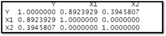
The diagnostic aids show that firstly, there are no outliers and the distribution for each variable is normal. Additionally, looking at the correlation matrix, Y and X1 have significant positive correlation, Y and X2 are positively correlated, but less so than Y and X1 and there’s no correlation between X1 and X2.

Correlation Matrix:

The correlation matrix of the variables is plotted to check the correlation between the variables.

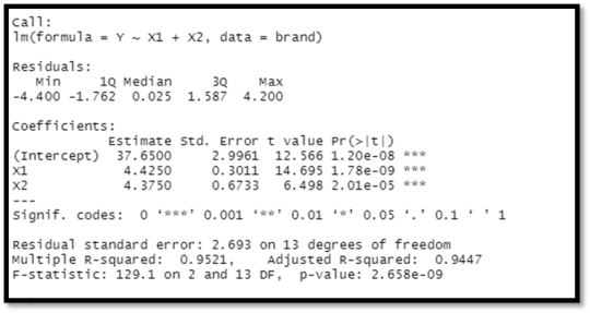
Summary:

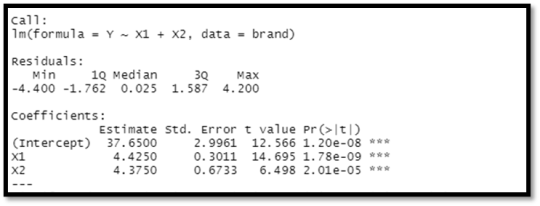
The value of multiple R- squared is 0.9521 and the adjusted R- squared value is 0.9447. When the variable X2, is added to X1 we get a p-value of about 2.01e-05. F- statistic variable is larger than 1. Y= 37.65 + 4.425X1 + 4.375X2 is the result of the regression model. Holding the other variables constant, increasing one unit of X1 results in a 4.425 rise in brand liking degree, while increasing one unit of X2 results in a 4.375 increase in brand liking degree. Because the P values for each variable are less than 0.05, both X1 and X2 are significant.

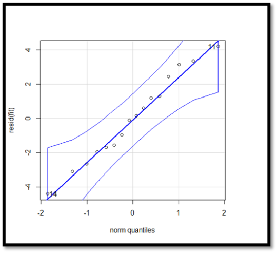
QQ plot:

In this QQ- plot the points plotted all fall in the same line which clearly determines that the residuals follow normal distribution. There are no outliers and errors .

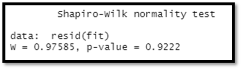
Shapiro test:

Shapiro Wilk test is a statistic normality test for a random data set. It can be used to analyse if the data set is normally distributed. By analysing the values, we get,

Model validation:

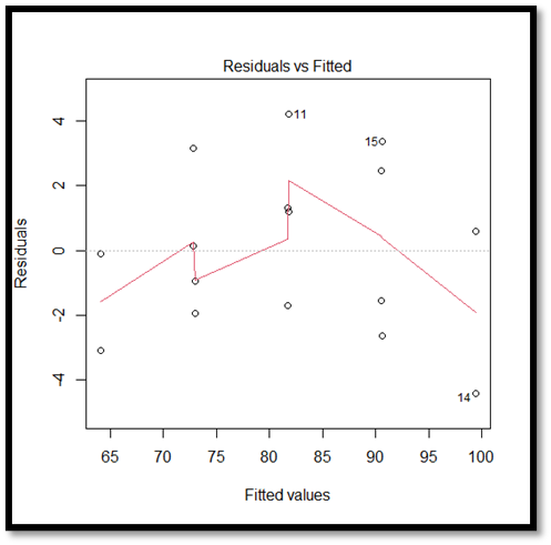
Regression vs Residual Plot:

The above given plot is a residual plot which indicates a pattern in the residuals and the fitted plot. Although the distribution appears to be pretty normal, there are outliers on both sides of the median, with more outliers to the right.

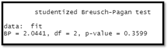
Breusch-Pagan test:

This is test can be used to determine whether the heteroscedasticity is present in a regression analysis

Prediction and Confidence level:

newX = data. frame (X1=newX1, X2 = newX2)

#Confidence interval (95%)

predict (fit, newX, interval="confidence")

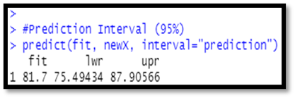
#Prediction Interval (95%)

predict (fit, newX, interval="prediction"

Output:

Interpretation:

From the above analysis, we get that the R- square is about 95% is very good and the results are accurate and the overall relationship is significant.

[regressingnow]

Working with Multiple Regression : W3

Regression Modeling In Practice 3

In the third week of our assignments at Regression Modeling in Practice, we were expected to perform a multiple regression model between an initial explanatory variable from a large dataset, and add several other confounding variables to improve the prediction capabilities.

I continued to use the ‘gapminder’ dataset from last week which provides data about the population, life expectancy and GDP in different countries of the world from 1952 to 2007. Within this large dataset, We already examined a possible relationship between the Per Capita Income in a country versus it’s life expectancy. Now we will look at effect of other confounding variables which could provide a better prediction of the Life Expectancy in the country

Experiment

It is logically expected that a higher income provides access to better healthcare, increases affordability of prescription drugs, and possibly access to better insurance policies, thus improving life expectancy. This was the reason to choose the Per Capita Income as the first explanatory variable. However, there are several other factors in the dataset which might contribute to the life expectancy in a particular country. Factors such as ‘Alcohol Consumption’, ‘Employment Rate’, and ‘Urbanization Rate’ all do definitely affect the life expectancy of a single person and a country as a whole. Let’s examine if the data says the same too. 

Details

Here, the ‘Income Per Person’ is the primary explanatory variable while the ‘Life Expectancy’ becomes the response variable. 

A Linear Regression Model of  ‘Income Per Person’ and  ‘Life Expectancy’ gives the following result :

Mean for Income Per Person 7262.857778727173 Mean for Centered Income Per Person 6.025402399245649e-13

From the R-Squared values reported in the OLS Model, we can understand that about 36.7% of the variance seen in the Life Expectancy can be attributed to the Per Capita Income.

The p-value is very small <0.0001, this indicating that the null hypothesis can be rejected. There is indeed a significant effect of Per Capita Income on the Life Expectancy. Beta is 0.0006.

Life Expectancy = 0.0006*(Centered Income Per Person)+72.2992 

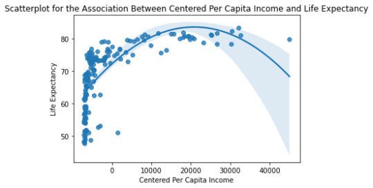
However, a plot between the Per Capita Income and Life Expectancy does not show a great agreement between the model prediction and available data, especially at lower Per Capita Income (PCI).

Scatter for the Linear association between Life Expectancy and PCI

Using  a 2nd order Quadratic Regression Model for the same two variables, we get the following result :

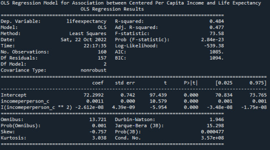
We get a better R-Squared value reported in the OLS Model of 0.484, thus proving a better fit, as seen in the plot below. Beta value of 0.0011 is also to be noted.

The p-value is very small <0.0001, this indicating that the null hypothesis can be rejected. There is indeed a significant effect of Per Capita Income on the Life Expectancy.

Life Expectancy = -2.6e-8*( (Centered Income Per Person)^2 + 0.0011*(Centered Income Per Person) + 72.299

We will retain this quadratic relationship for the Multiple Regression too

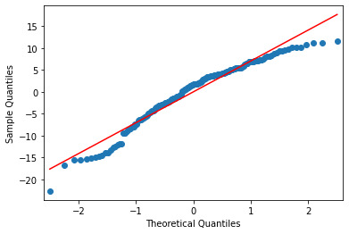
Below is the qq-plot for the quadratic regression model. There are some outliers at the lower and higher ends of the data.

And here is the residual plot. There are more outliers towards the negative residuals but not significantly high.

Let us now analyze ‘Alcohol Consumption’ as the first confounding variable while the ‘Life Expectancy’ becomes the response variable.

A Linear Regression Model of  ‘Alcohol Consumption’ and  ‘Life Expectancy’ gives the following result :

Mean for Alcohol Consumption 6.824312499999998 Mean for Centered Alcohol Consumption 2.2398749521812534e-15

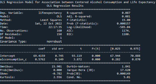
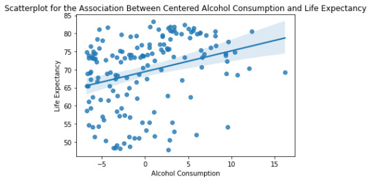
From the R-Squared values reported in the OLS Model, we can understand that about 8.7% of the variance seen in the Life Expectancy can be attributed to the Alcohol Consumption. There is a positive-Beta value of 0.5762

The p-value is very small <0.0001, this indicating that the null hypothesis can be rejected. There is indeed a significant effect of Alcohol Consumption on the Life Expectancy.

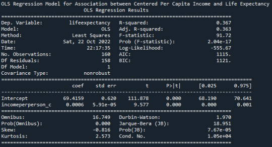
Life Expectancy = 0.5762*(Centered Alcohol Consumption)+69.4159

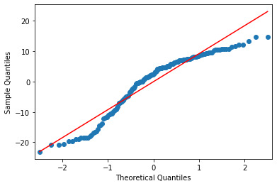
Below is the qq-plot for the quadratic regression model. Some of the lower outliers from the previous case are better accounted here.

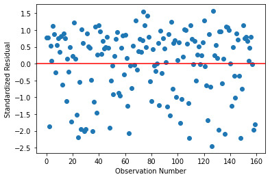
And once again the residual plot is as below. Once again,  there are more outliers towards the negative residuals but not significantly large number.

Let us now further analyze ‘Employment Rate’ as the second confounding variable while the ‘Life Expectancy’ becomes the response variable.

A Linear Regression Model of  ‘ Employment Rate ’ and  ‘Life Expectancy’ gives the following result :

Mean for Employment Rate 59.076875066757204 Mean for Centered Employment Rate -5.773159728050814e-16

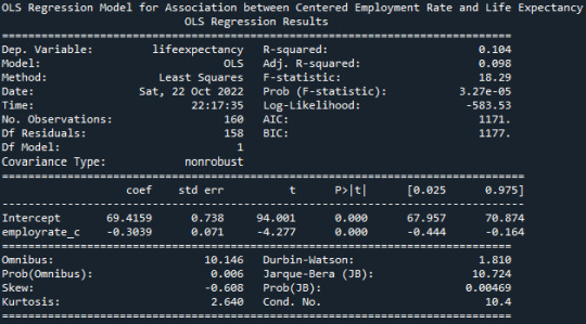
From the R-Squared values reported in the OLS Model, we can understand that about 10.4% of the variance seen in the Life Expectancy can be attributed to the Alcohol Consumption. There is a negative-Beta value of 0.3039, suggesting that the Life Expectancy decreases with the Employment Rate.

The p-value is very small <0.0001, this indicating that there is indeed a significant effect of Employment Rate on the Life Expectancy.

Life Expectancy = -0.3039*(Centered Employment Rate)+69.4159

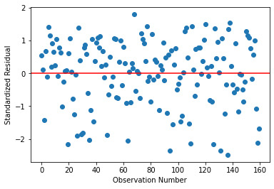
Below is the qq-plot for the quadratic regression model. Again some of the lower outliers from the previous case are better accounted here., and it has a better agreement along the center portion too

Here is the corresponding Residual Plot

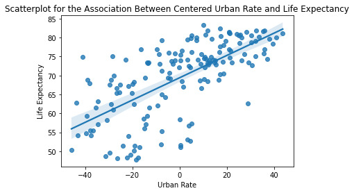
Finally, et us  analyze ‘Urbanization Rate’ as the last confounding variable while the ‘Life Expectancy’ becomes the response variable.

A Linear Regression Model of  ‘Urbanization Rate ’ and  ‘Life Expectancy’ gives the following result :

Mean for Urban Rate 56.278125 Mean for Centered Urban Rate -2.3092638912203257e-15

From the R-Squared values reported in the OLS Model, we can understand that about 44% of the variance seen in the Life Expectancy can be attributed to the Alcohol Consumption. There is a positive-Beta value of 0.2940.

The p-value is very small <0.0001, this indicating that there is indeed a significant effect of Urbanization Rate on the Life Expectancy.

Life Expectancy = 0.2940*(Centered Urbanization Rate)+69.4159

Below is the qq-plot for the quadratic regression model. This is one of the best agreements seen in this analysis.

And once again, the corresponding Residual Plot. As suggested by the fit, the outliers are also limited with this model.

Multiple Regression Model using the above variables for ’Life Expectancy’ Response Variable

Using the above gathered variables, both explanatory and confounding, in a multiple regression analysis, we get the following output

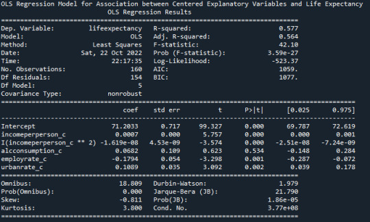
Evaluating the Model Fit for all the variables, we see the following

From the P-values (P < 0.05) for each of the individual explanatory and confounding variables, it is evident that Income per Person (Beta = 0.0007), Employment Rate (Beta = -0.1794) , and Urbanization rate  (Beta = 0.1089) ave a strong association with the Life Expectancy in a country. However, Alcohol Consumption (P-Value > 0.05) has no effect on the Life Expectancy. The overall R-Squared value of 0.577 indicates that about 57.7 percent of the variance in the Life Expectancy can be explained by the Per Capita Income, Employment Rate, and Urbanization Rate.

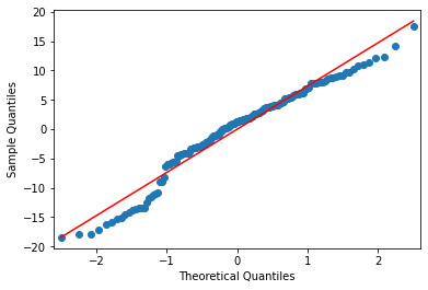
The qq plot below, for the multiple regression continues to show outliers at the lower and upper ends, but shows a pretty agreement otherwise.

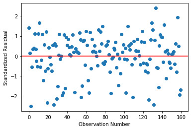
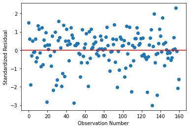
Below is the residual plot from Multiple Regression Analysis. Much of the residuals do lie within 1 standard deviation, while some are present between -1 and -2 standard deviation too. The fit could be made better by the addition of other explanatory variables.

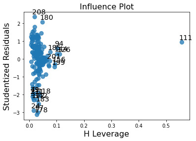
Below is the Leverage Plot for the Multiple Regression Model. This plot also tells us that the outliers have small or close to zero leverage values, meaning that although they are outlying observations, they do not have an undue influence on the estimation of the regression model. The one observation that has a large leverage on the model is however not an outlier.

Thus, we have successfully formulated a Multiple Regression Model that can explain upto 60% of the variance in Life Expectancy using a combination of explanatory variables.

Below is the Code that was used to generate these results :

mainset[["employrate_c"]]=mainset[["employrate"]]-mainset[["employrate"]].mean() mainset[["urbanrate_c"]]=mainset[["urbanrate"]]-mainset[["urbanrate"]].mean()

#Collecting the Variables ppincome = mainset.incomeperperson ppincome_c = mainset.incomeperperson_c alcohol = mainset.alcconsumption alcohol_c = mainset.alcconsumption_c co2emit = mainset.co2emissions co2emit_c = mainset.co2emissions_c emprate = mainset.employrate emprate_c = mainset.employrate_c urbrate = mainset.urbanrate urbrate_c = mainset.urbanrate_c lifeyears = mainset.lifeexpectancy

#Basic Linear Regression with centered Income Per Person print ("Mean for Income Per Person") meanppi = ppincome.mean() print(meanppi) print ("Mean for Centered Income Per Person") meanppi_c = ppincome_c.mean() print(meanppi_c)

#Basic Linear Regression with centered Income Per Person (Linear) print('OLS Regression Model for Association between Centered Per Capita Income and Life Expectancy') reg1 = smf.ols('lifeexpectancy ~ incomeperperson_c',data=mainset).fit() print(reg1.summary())

#Plotting the explanatory centered Income Per Person and Life Expectancy (Linear) scat1 = seaborn.regplot(x="incomeperperson_c", y="lifeexpectancy", scatter=True, data=mainset) plt.xlabel('Centered Per Capita Income') plt.ylabel('Life Expectancy') plt.title ('Scatterplot for the Association Between Centered Per Capita Income and Life Expectancy') print(scat1)

#Basic Quadratic Regression with centered Income Per Person print('OLS Regression Model for Association between Centered Per Capita Income and Life Expectancy') reg2 = smf.ols('lifeexpectancy ~ incomeperperson_c+ I(incomeperperson_c**2)',data=mainset).fit() print(reg2.summary())

#Plotting the explanatory centered Income Per Person and Life Expectancy (2nd Order) scat2 = seaborn.regplot(x="incomeperperson_c", y="lifeexpectancy", scatter=True, order =2, data=mainset) plt.xlabel('Centered Per Capita Income') plt.ylabel('Life Expectancy') plt.title ('Scatterplot for the Association Between Centered Per Capita Income and Life Expectancy') print(scat2)

#Q-Q plot for normality fig1=sm.qqplot(reg2.resid, line='r')

# simple plot of residuals stdres1=pd.DataFrame(reg2.resid_pearson) plt.plot(stdres1, 'o', ls='None') l = plt.axhline(y=0, color='r') plt.ylabel('Standardized Residual') plt.xlabel('Observation Number')

#Basic Linear Regression with centered Alcohol Consumption print ("Mean for Alcohol Consumption") meanalc = alcohol.mean() print(meanalc) print ("Mean for Centered Alcohol Consumption") meanalc_c = alcohol_c.mean() print(meanalc_c)

#Basic Linear Regression with centered Alcohol Consumption (Linear) print('OLS Regression Model for Association between Centered Alcohol Consumption and Life Expectancy') reg3 = smf.ols('lifeexpectancy ~ alcconsumption_c',data=mainset).fit() print(reg3.summary())

#Plotting the explanatory centered Alcohol Consumption and Life Expectancy scat3 = seaborn.regplot(x="alcconsumption_c", y="lifeexpectancy", scatter=True, data=mainset) plt.xlabel('Alcohol Consumption') plt.ylabel('Life Expectancy') plt.title ('Scatterplot for the Association Between Centered Alcohol Consumption and Life Expectancy') print(scat3)

#Q-Q plot for normality fig2=sm.qqplot(reg3.resid, line='r')

# simple plot of residuals stdres2=pd.DataFrame(reg3.resid_pearson) plt.plot(stdres2, 'o', ls='None') l = plt.axhline(y=0, color='r') plt.ylabel('Standardized Residual') plt.xlabel('Observation Number')

#Basic Linear Regression with centered Employment Rate print ("Mean for Employment Rate") meanemp = emprate.mean() print(meanemp) print ("Mean for Centered Employment Rate") meanemp_c = emprate_c.mean() print(meanemp_c)

#Basic Linear Regression with centered Emplotment Rate (Linear) print('OLS Regression Model for Association between Centered Employment Rate and Life Expectancy') reg4 = smf.ols('lifeexpectancy ~ employrate_c',data=mainset).fit() print(reg4.summary())

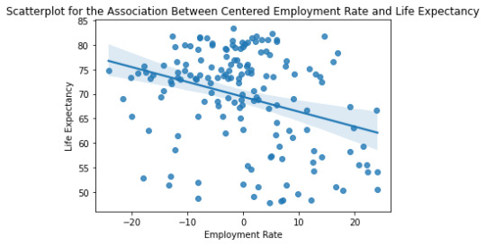
#Plotting the explanatory centered Empoyment Rate and Life Expectancy scat4 = seaborn.regplot(x="employrate_c", y="lifeexpectancy", scatter=True, data=mainset) plt.xlabel('Employment Rate') plt.ylabel('Life Expectancy') plt.title ('Scatterplot for the Association Between Centered Employment Rate and Life Expectancy') print(scat4)

#Q-Q plot for normality fig3=sm.qqplot(reg4.resid, line='r')

# simple plot of residuals stdres3=pd.DataFrame(reg4.resid_pearson) plt.plot(stdres3, 'o', ls='None') l = plt.axhline(y=0, color='r') plt.ylabel('Standardized Residual') plt.xlabel('Observation Number')

#Basic Linear Regression with centered Urban Rate print ("Mean for Urban Rate") meanurb = urbrate.mean() print(meanurb) print ("Mean for Centered AUrban Rate") meanurb_c = urbrate_c.mean() print(meanurb_c)

#Basic Linear Regression with centered Urban Rate (Linear) print('OLS Regression Model for Association between Centered Urban Rate and Life Expectancy') reg5 = smf.ols('lifeexpectancy ~ urbanrate_c',data=mainset).fit() print(reg5.summary())

#Plotting the explanatory centered Urban Rate and Life Expectancy scat5 = seaborn.regplot(x="urbanrate_c", y="lifeexpectancy", scatter=True, data=mainset) plt.xlabel('Urban Rate') plt.ylabel('Life Expectancy') plt.title ('Scatterplot for the Association Between Centered Urban Rate and Life Expectancy') print(scat5)

#Q-Q plot for normality fig4=sm.qqplot(reg5.resid, line='r')

# simple plot of residuals stdres4=pd.DataFrame(reg5.resid_pearson) plt.plot(stdres4, 'o', ls='None') l = plt.axhline(y=0, color='r') plt.ylabel('Standardized Residual') plt.xlabel('Observation Number')

#Multiple Regression with centered Variables print('OLS Regression Model for Association between Centered Explanatory Variables and Life Expectancy') reg6 = smf.ols('lifeexpectancy ~ incomeperperson_c+ I(incomeperperson_c**2)+alcconsumption_c+employrate_c+urbanrate_c',data=mainset).fit() print(reg6.summary())

#Q-Q plot for normality fig5=sm.qqplot(reg6.resid, line='r')

# simple plot of residuals stdres5=pd.DataFrame(reg6.resid_pearson) plt.plot(stdres5, 'o', ls='None') l = plt.axhline(y=0, color='r') plt.ylabel('Standardized Residual') plt.xlabel('Observation Number')

# leverage plot fig6=sm.graphics.influence_plot(reg6, size=8) print(fig6)

# additional regression diagnostic plots fig7 = plt.figure(figsize=(12,8)) fig7 = sm.graphics.plot_regress_exog(reg6,  "incomeperperson_c", fig=fig7)

fig8 = plt.figure(figsize=(12,8)) fig8 = sm.graphics.plot_regress_exog(reg6,  "employrate_c", fig=fig8)

fig9 = plt.figure(figsize=(12,8)) fig9 = sm.graphics.plot_regress_exog(reg6,  "urbanrate_c", fig=fig9)

fig10 = plt.figure(figsize=(12,8)) fig10 = sm.graphics.plot_regress_exog(reg6,  "alcconsumption_c", fig=fig10)

[rohanms]

Multiple Regression using Marketing Field

Multiple linear regression:

A multiple linear regression is an extension of a simple linear regression and uses separate predictor variables (x) to predict the outcome variable (y). With 3 predictor variables (x), the prediction of y is expressed as:

y = b0 + b1*x1 + b2*x2 + b3*x3

The b is called the beta coefficients. We will now build, interpret a multiple linear regression model in R & check the overall quality of the model.

install.packages('tidyverse')

We will use the marketing data set [datarium package] to determine which advertising mediums (youtube, facebook, and newspaper) are associated with sales.

data("marketing", package = "datarium")

head(marketing, 4)

My dataset consists of 3 independent variables:

1. YouTube

2. Facebook

3. Newspaper

The dependent variable is the Sales variable. This study was designed to investigate what effect ads from different platforms have on sales.

BUILDING MODEL

Using the advertising budget invested in youtube, facebook, and newspapers, we want to estimate sales as follows:

sales = b0 + b1*youtube + b2*facebook + b3*newspaper

In R, the model coefficients can be computed as follows:

model <- lm(sales ~ youtube + facebook + newspaper, data = marketing)

summary(model)

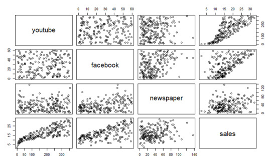
plot(marketing)

INTERPRETATION

Taking a look at the F-statistic and the associated p-value, which are provided on the model summary, is the first step in interpreting the multiple regression analysis.

We see that the F-statistic has a significant p-value of 2.2e-16 in our example. A significant relationship exists between one of the predictor variables and the outcome variable, at least.

The coefficients table shows the estimated beta coefficients and the associated t-statistic p-values, so you can determine which predictor variables are significant:

summary(model)$coefficient

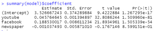
By looking at the t-statistic for a given predictor, we can determine whether there is a significant difference between the beta coefficient of the predictor and the outcome variable. Changing advertising budgets for YouTube and Facebook are significantly correlated with changes in sales, while changing newspaper budgets are not significantly correlated with sales.

The coefficient (b) can be interpreted as the overall effect of an increase in a predictor variable of one unit held constant, when all other predictors are held constant.

A YouTube and newspaper advertising budget of $1000 each result in an increase of 189 units of sales, on average, when you spend an additional $1,000 on facebook advertising. According to the YouTube coefficient, for every $1000 increase in YouTube advertising budget, all other factors being equal, 45 sales units will increase on average for each $1000 increase.

In our multiple regression analysis, newspaper was not significant. Accordingly, a change in the newspaper advertising budget will not have a significant impact on sales units when YouTube and newspaper advertising budgets are both fixed.

In this case, we may remove the newspaper variable since it is not significant:

model <- lm(sales ~ youtube + facebook, data = marketing)

summary(model)

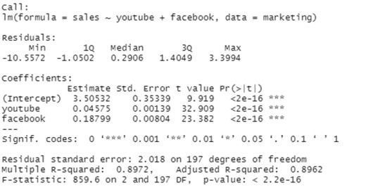
Finally, our model equation can be written as follow:

sales = 3.5 + 0.045*youtube + 0.187*facebook

The confidence interval of the model coefficient can be extracted as follow:

confint(model)

The R-squared (R2) and Residual Standard Error (RSE) can be used to assess the overall quality of a model, as we have already seen in simple linear regression.

R-squared:

The correlation coefficient R2 in multiple linear regression reflects the relationship between the observed (or actual) values of the outcome variable (y) and the predicted (or fitted) values of y. In this case, R will always have a positive value and will range from zero to one. Based on the x variables, R2 represents the proportion of variance that can be predicted in the outcome variable y. The value of R2 close to 1 indicates that the model can explain a large proportion of the variance in the outcome variable. When more variables are added to the model, the R2 will always increase, even if those variables are only weakly associated with the response. By taking the number of predictor variables into account, the R2 can be adjusted.

In the summary output, the adjustment in the "Adjusted R Square" value corresponds to the number of x variables in the prediction model.

The adjusted R2 in our example, with YouTube and Facebook as predictor variables, is 0.89, meaning that youtube and Facebook advertising budgets are capable of predicting 89% of the variance in sales.

The adjusted R2 of 0.61 is better than the simple linear model with only YouTube.

Residual Standard Error (RSE):

It is also called as the sigma. The RSE estimate gives a measure of error of prediction. In general, a model with a lower RSE is more accurate (on the data in hand).

By dividing the RSE by the mean outcome variable, the error rate can be estimated:

sigma(model)/mean(marketing$sales)

The RSE for our multiple regression example is 2.023, which translates to a 12% error rate.

As a result, the RSE is 3.9 (*23% error rate) for the simple model, with only the youtube variable.

This work is done by

Rohan M

MBA (2020-2022)

Amrita School of Business

Coimbatore

NOTE:  “This blog is a part of the assignments done in the course Data Analysis using R and Python".

[taliemsite-blog]

(via Transformational leadership | سایت آموزشی تعلیم) Purpose – The purpose of this paper is to investigate the mechanisms that link transformational leadership to employee job satisfaction by examining the moderating effect of contingent reward on the relationships. Design/methodology/approach – The study employed explanatory and cross-sectional survey design. Data were obtained from 315 bank employees and analyzed using correlational and multipleregression techniques. Findings – The results revealed that there are positive relationships between the dimensions of transformational leadership and job satisfaction which are augmented by contingent reward. However, the relationships of idealized influence and intellectual simulation to job satisfaction are moderated by contingent reward, implying that, in the banking sector, the positive influence of these transformational leadership traits on employee job satisfaction can be enhanced by contingent reward. Originality/value – The paper makes an important contribution to the existing organizational literature by establishing the utility of contingent reward as a moderator on the relationship between transformational leadership and employee job satisfaction in a banking sector. #psychology #mechanisms  #leadership  

[letsreliabletermpapersblr-blog]

Multiple Regression and Correlation Analysis

Multiple Regression and Correlation Analysis

MultipleRegression and Correlation Analysis ProjectGeneral information1. This project is worth 15%.2. The majority of the calculation and data analysis will be done using MegaStat, SPSS or Minitab or other software.3.ÿÿ ÿThe penalty for a late project is 3 marks per day. Your mark for the project will be zero after 5 working days. You are, however, still required to hand in a satisfactory…

[taliemsite-blog]

Purpose – The purpose of this paper is to investigate the mechanisms that link transformational leadership to employee job satisfaction by examining the moderating effect of contingent reward on the relationships. Design/methodology/approach – The study employed explanatory and cross-sectional survey design. Data were obtained from 315 bank employees and analyzed using correlational and multipleregression techniques. Findings – The results revealed that there are positive relationships between the dimensions of transformational leadership and job satisfaction which are augmented by contingent reward. However, the relationships of idealized influence and intellectual simulation to job satisfaction are moderated by contingent reward, implying that, in the banking sector, the positive influence of these transformational leadership traits on employee job satisfaction can be enhanced by contingent reward. Originality/value – The paper makes an important contribution to the existing organizational literature by establishing the utility of contingent reward as a moderator on the relationship between transformational leadership and employee job satisfaction in a banking sector.

#psychology #employee  #mechanisms