#Python Pandas Data Frames | Explore Tumblr posts and blogs

vivekavicky12 · 2 years ago

Text

From Math to Machine Learning: A Comprehensive Blueprint for Aspiring Data Scientists

The realm of data science is vast and dynamic, offering a plethora of opportunities for those willing to dive into the world of numbers, algorithms, and insights. If you're new to data science and unsure where to start, fear not! This step-by-step guide will navigate you through the foundational concepts and essential skills to kickstart your journey in this exciting field. Choosing the Best Data Science Institute can further accelerate your journey into this thriving industry.

1. Establish a Strong Foundation in Mathematics and Statistics

Before delving into the specifics of data science, ensure you have a robust foundation in mathematics and statistics. Brush up on concepts like algebra, calculus, probability, and statistical inference. Online platforms such as Khan Academy and Coursera offer excellent resources for reinforcing these fundamental skills.

2. Learn Programming Languages

Data science is synonymous with coding. Choose a programming language – Python and R are popular choices – and become proficient in it. Platforms like Codecademy, DataCamp, and W3Schools provide interactive courses to help you get started on your coding journey.

3. Grasp the Basics of Data Manipulation and Analysis

Understanding how to work with data is at the core of data science. Familiarize yourself with libraries like Pandas in Python or data frames in R. Learn about data structures, and explore techniques for cleaning and preprocessing data. Utilize real-world datasets from platforms like Kaggle for hands-on practice.

4. Dive into Data Visualization

Data visualization is a powerful tool for conveying insights. Learn how to create compelling visualizations using tools like Matplotlib and Seaborn in Python, or ggplot2 in R. Effectively communicating data findings is a crucial aspect of a data scientist's role.

5. Explore Machine Learning Fundamentals

Begin your journey into machine learning by understanding the basics. Grasp concepts like supervised and unsupervised learning, classification, regression, and key algorithms such as linear regression and decision trees. Platforms like scikit-learn in Python offer practical, hands-on experience.

6. Delve into Big Data Technologies

As data scales, so does the need for technologies that can handle large datasets. Familiarize yourself with big data technologies, particularly Apache Hadoop and Apache Spark. Platforms like Cloudera and Databricks provide tutorials suitable for beginners.

7. Enroll in Online Courses and Specializations

Structured learning paths are invaluable for beginners. Enroll in online courses and specializations tailored for data science novices. Platforms like Coursera ("Data Science and Machine Learning Bootcamp with R/Python") and edX ("Introduction to Data Science") offer comprehensive learning opportunities.

8. Build Practical Projects

Apply your newfound knowledge by working on practical projects. Analyze datasets, implement machine learning models, and solve real-world problems. Platforms like Kaggle provide a collaborative space for participating in data science competitions and showcasing your skills to the community.

9. Join Data Science Communities

Engaging with the data science community is a key aspect of your learning journey. Participate in discussions on platforms like Stack Overflow, explore communities on Reddit (r/datascience), and connect with professionals on LinkedIn. Networking can provide valuable insights and support.

10. Continuous Learning and Specialization

Data science is a field that evolves rapidly. Embrace continuous learning and explore specialized areas based on your interests. Dive into natural language processing, computer vision, or reinforcement learning as you progress and discover your passion within the broader data science landscape.

Remember, your journey in data science is a continuous process of learning, application, and growth. Seek guidance from online forums, contribute to discussions, and build a portfolio that showcases your projects. Choosing the best Data Science Courses in Chennai is a crucial step in acquiring the necessary expertise for a successful career in the evolving landscape of data science. With dedication and a systematic approach, you'll find yourself progressing steadily in the fascinating world of data science. Good luck on your journey!

#data science certification #data science course #data science training #datascience #technology

3 notes · View notes

xaltius · 10 days ago

Text

ChatGPT & Data Science: Your Essential AI Co-Pilot

The rise of ChatGPT and other large language models (LLMs) has sparked countless discussions across every industry. In data science, the conversation is particularly nuanced: Is it a threat? A gimmick? Or a revolutionary tool?

The clearest answer? ChatGPT isn't here to replace data scientists; it's here to empower them, acting as an incredibly versatile co-pilot for almost every stage of a data science project.

Think of it less as an all-knowing oracle and more as an exceptionally knowledgeable, tireless assistant that can brainstorm, explain, code, and even debug. Here's how ChatGPT (and similar LLMs) is transforming data science projects and how you can harness its power:

How ChatGPT Transforms Your Data Science Workflow

Problem Framing & Ideation: Struggling to articulate a business problem into a data science question? ChatGPT can help.

"Given customer churn data, what are 5 actionable data science questions we could ask to reduce churn?"

"Brainstorm hypotheses for why our e-commerce conversion rate dropped last quarter."

"Help me define the scope for a project predicting equipment failure in a manufacturing plant."

Data Exploration & Understanding (EDA): This often tedious phase can be streamlined.

"Write Python code using Pandas to load a CSV and display the first 5 rows, data types, and a summary statistics report."

"Explain what 'multicollinearity' means in the context of a regression model and how to check for it in Python."

"Suggest 3 different types of plots to visualize the relationship between 'age' and 'income' in a dataset, along with the Python code for each."

Feature Engineering & Selection: Creating new, impactful features is key, and ChatGPT can spark ideas.

"Given a transactional dataset with 'purchase_timestamp' and 'product_category', suggest 5 new features I could engineer for a customer segmentation model."

"What are common techniques for handling categorical variables with high cardinality in machine learning, and provide a Python example for one."

Model Selection & Algorithm Explanation: Navigating the vast world of algorithms becomes easier.

"I'm working on a classification problem with imbalanced data. What machine learning algorithms should I consider, and what are their pros and cons for this scenario?"

"Explain how a Random Forest algorithm works in simple terms, as if you're explaining it to a business stakeholder."

Code Generation & Debugging: This is where ChatGPT shines for many data scientists.

"Write a Python function to perform stratified K-Fold cross-validation for a scikit-learn model, ensuring reproducibility."

"I'm getting a 'ValueError: Input contains NaN, infinity or a value too large for dtype('float64')' in my scikit-learn model. What are common reasons for this error, and how can I fix it?"

"Generate boilerplate code for a FastAPI endpoint that takes a JSON payload and returns a prediction from a pre-trained scikit-learn model."

Documentation & Communication: Translating complex technical work into understandable language is vital.

"Write a clear, concise docstring for this Python function that preprocesses text data."

"Draft an executive summary explaining the results of our customer churn prediction model, focusing on business impact rather than technical details."

"Explain the limitations of an XGBoost model in a way that a non-technical manager can understand."

Learning & Skill Development: It's like having a personal tutor at your fingertips.

"Explain the concept of 'bias-variance trade-off' in machine learning with a practical example."

"Give me 5 common data science interview questions about SQL, and provide example answers."

"Create a study plan for learning advanced topics in NLP, including key concepts and recommended libraries."

Important Considerations and Best Practices

While incredibly powerful, remember that ChatGPT is a tool, not a human expert.

Always Verify: Generated code, insights, and especially factual information must always be verified. LLMs can "hallucinate" or provide subtly incorrect information.

Context is King: The quality of the output directly correlates with the quality and specificity of your prompt. Provide clear instructions, examples, and constraints.

Data Privacy is Paramount: NEVER feed sensitive, confidential, or proprietary data into public LLMs. Protecting personal data is not just an ethical imperative but a legal requirement globally. Assume anything you input into a public model may be used for future training or accessible by the provider. For sensitive projects, explore secure, on-premises or private cloud LLM solutions.

Understand the Fundamentals: ChatGPT is an accelerant, not a substitute for foundational knowledge in statistics, machine learning, and programming. You need to understand why a piece of code works or why an an algorithm is chosen to effectively use and debug its outputs.

Iterate and Refine: Don't expect perfect results on the first try. Refine your prompts based on the output you receive.

ChatGPT and its peers are fundamentally changing the daily rhythm of data science. By embracing them as intelligent co-pilots, data scientists can boost their productivity, explore new avenues, and focus their invaluable human creativity and critical thinking on the most complex and impactful challenges. The future of data science is undoubtedly a story of powerful human-AI collaboration.

#technology #artificial intelligence #ai #online course #data science course #data science #chatgpt

0 notes

pabloatech · 19 days ago

Text

4th week: plotting variables

I put here as usual the python script, the results and the comments:

Python script:

Created on Tue Jun 3 09:06:33 2025

@author: PabloATech """

libraries/packages

import pandas import numpy import seaborn import matplotlib.pyplot as plt

read the csv table with pandas:

data = pandas.read_csv('C:/Users/zop2si/Documents/Statistic_tests/nesarc_pds.csv', low_memory=False)

show the dimensions of the data frame:

print() print ("length of the dataframe (number of rows): ", len(data)) #number of observations (rows) print ("Number of columns of the dataframe: ", len(data.columns)) # number of variables (columns)

variables:

variable related to the background of the interviewed people (SES: socioeconomic status):

biological/adopted parents got divorced or stop living together before respondant was 18

data['S1Q2D'] = pandas.to_numeric(data['S1Q2D'], errors='coerce')

variable related to alcohol consumption

HOW OFTEN DRANK ENOUGH TO FEEL INTOXICATED IN LAST 12 MONTHS

data['S2AQ10'] = pandas.to_numeric(data['S2AQ10'], errors='coerce')

variable related to the major depression (low mood I)

EVER HAD 2-WEEK PERIOD WHEN FELT SAD, BLUE, DEPRESSED, OR DOWN MOST OF TIME

data['S4AQ1'] = pandas.to_numeric(data['S4AQ1'], errors='coerce')

NUMBER OF EPISODES OF PATHOLOGICAL GAMBLING

data['S12Q3E'] = pandas.to_numeric(data['S12Q3E'], errors='coerce')

HIGHEST GRADE OR YEAR OF SCHOOL COMPLETED

data['S1Q6A'] = pandas.to_numeric(data['S1Q6A'], errors='coerce')

Choice of thee variables to display its frequency tables:

string_01 = """ Biological/adopted parents got divorced or stop living together before respondant was 18: 1: yes 2: no 9: unknown -> deleted from the analysis blank: unknown """

string_02 = """ HOW OFTEN DRANK ENOUGH TO FEEL INTOXICATED IN LAST 12 MONTHS

Every day

Nearly every day

3 to 4 times a week

2 times a week

Once a week

2 to 3 times a month

Once a month

7 to 11 times in the last year

3 to 6 times in the last year

1 or 2 times in the last year

Never in the last year

Unknown -> deleted from the analysis BL. NA, former drinker or lifetime abstainer """

string_02b = """ HOW MANY DAYS DRANK ENOUGH TO FEEL INTOXICATED IN THE LAST 12 MONTHS: """

string_03 = """ EVER HAD 2-WEEK PERIOD WHEN FELT SAD, BLUE, DEPRESSED, OR DOWN MOST OF TIME:

Yes

Unknown -> deleted from the analysis """

string_04 = """ NUMBER OF EPISODES OF PATHOLOGICAL GAMBLING """

string_05 = """ HIGHEST GRADE OR YEAR OF SCHOOL COMPLETED

No formal schooling

Completed grade K, 1 or 2

Completed grade 3 or 4

Completed grade 5 or 6

Completed grade 7

Completed grade 8

Some high school (grades 9-11)

Completed high school

Graduate equivalency degree (GED)

Some college (no degree)

Completed associate or other technical 2-year degree

Completed college (bachelor's degree)

Some graduate or professional studies (completed bachelor's degree but not graduate degree)

Completed graduate or professional degree (master's degree or higher) """

replace unknown values for NaN and remove blanks

data['S1Q2D']=data['S1Q2D'].replace(9, numpy.nan) data['S2AQ10']=data['S2AQ10'].replace(99, numpy.nan) data['S4AQ1']=data['S4AQ1'].replace(9, numpy.nan) data['S12Q3E']=data['S12Q3E'].replace(99, numpy.nan) data['S1Q6A']=data['S1Q6A'].replace(99, numpy.nan)

create a recode for number of intoxications in the last 12 months:

recode1 = {1:365, 2:313, 3:208, 4:104, 5:52, 6:36, 7:12, 8:11, 9:6, 10:2, 11:0} data['S2AQ10'] = data['S2AQ10'].map(recode1)

print(" ") print("Statistical values for varible 02 alcohol intoxications of past 12 months") print(" ") print ('mode: ', data['S2AQ10'].mode()) print ('mean', data['S2AQ10'].mean()) print ('std', data['S2AQ10'].std()) print ('min', data['S2AQ10'].min()) print ('max', data['S2AQ10'].max()) print ('median', data['S2AQ10'].median()) print(" ") print("Statistical values for highest grade of school completed") print ('mode', data['S1Q6A'].mode()) print ('mean', data['S1Q6A'].mean()) print ('std', data['S1Q6A'].std()) print ('min', data['S1Q6A'].min()) print ('max', data['S1Q6A'].max()) print ('median', data['S1Q6A'].median()) print(" ")

plot01 = seaborn.countplot(x="S2AQ10", data=data) plt.xlabel('Alcohol intoxications past 12 months') plt.title('Alcohol intoxications in the Past 12 Months in the NESARC Study')

plot02 = seaborn.countplot(x="S1Q6A", data=data) plt.xlabel('Highest grade (1-14)') plt.title('Highest grade or year of school completed')

I create a copy of the data to be manipulated later

sub1 = data[['S2AQ10','S1Q6A']]

create bins for no intoxication, few intoxications, …

data['S2AQ10'] = pandas.cut(data.S2AQ10, [0, 6, 36, 52, 104, 208, 365], labels=["very few","some", "often", "quite often", "very often", "permanent"])

change format from numeric to categorical

data['S2AQ10'] = data['S2AQ10'].astype('category')

print ('intoxication category counts') c1 = data['S2AQ10'].value_counts(sort=False, dropna=True) print(c1)

bivariate bar graph C->Q

plot03 = seaborn.catplot(x="S2AQ10", y="S1Q6A", data=data, kind="bar", ci=None) plt.xlabel('Alcohol intoxications') plt.ylabel('Highest grade')

c4 = data['S1Q6A'].value_counts(sort=False, dropna=False) print("c4: ", c4) print(" ")

I do sth similar but the way around:

creating 3 level education variable

def edu_level_1 (row): if row['S1Q6A'] <9 : return 1 # high school if row['S1Q6A'] >8 and row['S1Q6A'] <13 : return 2 # bachelor if row['S1Q6A'] >12 : return 3 # master or higher

sub1['edu_level_1'] = sub1.apply (lambda row: edu_level_1 (row),axis=1)

change format from numeric to categorical

sub1['edu_level'] = sub1['edu_level'].astype('category')

plot04 = seaborn.catplot(x="edu_level_1", y="S2AQ10", data=sub1, kind="boxen") plt.ylabel('Alcohol intoxications in the past 12 months') plt.xlabel('Highest grade') plt.grid() plt.show()

Results and comments:

length of the dataframe (number of rows): 43093 Number of columns of the dataframe: 3008

Statistical values for variable "alcohol intoxications of past 12 months":

mode: 0 0.0 dtype: float64 mean 9.115493905630748 std 40.54485720135516 min 0.0 max 365.0 median 0.0

Statistical values for variable "highest grade of school completed":

mode 0 8 dtype: int64 mean 9.451024528345672 std 2.521281770664422 min 1 max 14 median 10.0

intoxication category counts very few 6026 some 2042 often 510 quite often 272 very often 184 permanent 276 Name: S2AQ10, dtype: int64

c4: (counts highest grade)

8 10935 6 1210 12 5251 14 3257 10 8891 13 1526 7 4518 11 3772 5 414 4 931 3 421 9 1612 2 137 1 218 Name: S1Q6A, dtype: int64

Plots: Univariate highest grade:

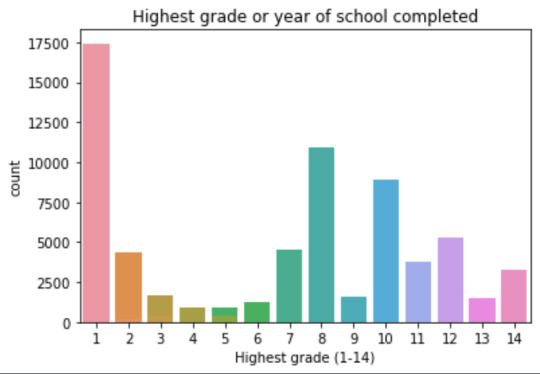
mean 9.45 std 2.5

-> mean and std. dev. are not very useful for this category-distribution. Most interviewed didn´t get any formal schooling, the next larger group completed the high school and the next one was at some college but w/o degree.

Univariate number of alcohol intoxications:

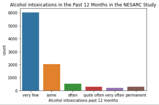
mean 9.12 std 40.54

-> very left skewed, most of the interviewed persons didn´t get intoxicated at all or very few times in the last 12 months (as expected)

Bivariate: the one against the other:

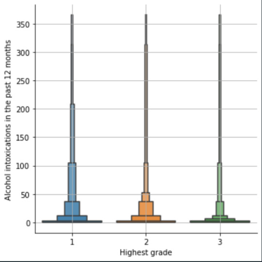
This bivariate plot shows three categories:

1: high school or lower

2: high school to bachelor

3: master or PhD

And the frequency of alcohol intoxications in the past 12 months.

The number of intoxications is higher in the group 1 for all the segments, but from 1 to 3 every group shows occurrences in any number of intoxications. More information and a more detailed analysis would be necessary to make conclusions.

0 notes

alivah2kinfosys · 4 months ago

Text

The Ultimate Selenium Training Guide: From Basics to Advanced

Introduction

In today’s fast-paced digital world, automation testing is no longer optional—it’s a necessity. Selenium is the industry leader in test automation, making it an essential skill for software testers and developers. Whether you’re a beginner or looking to advance your automation skills, this guide will walk you through everything you need to know about Selenium.

By the end of this guide, you’ll understand Selenium’s fundamentals, advanced techniques, and real-world applications, empowering you to excel in your career. If you're considering a Selenium certification course, this guide will also help you determine the right path for your learning journey.

What is Selenium?

Selenium is an open-source framework used for automating web applications. It supports multiple programming languages, browsers, and platforms, making it a flexible choice for automation testing.

Why is Selenium Important?

Cross-Browser Compatibility: Run tests on multiple browsers like Chrome, Firefox, and Edge.

Supports Multiple Programming Languages: Use Java, Python, C#, and more.

Integration with Other Tools: Works with TestNG, JUnit, and CI/CD pipelines.

Reduces Manual Testing Effort: Speeds up test execution and improves accuracy.

Getting Started with Selenium

Setting Up Selenium

To begin Selenium training online, you need the right setup. Follow these steps:

Install Java/Python: Choose a programming language for automation.

Download Selenium WebDriver: Get the necessary browser drivers.

Set Up an IDE: Use Eclipse, IntelliJ (for Java) or PyCharm (for Python).

Install Browser Drivers: Download ChromeDriver, GeckoDriver, etc.

Write Your First Test Script: Start with a simple test case.

Example of a simple Selenium script in Python:

from selenium import webdriver

# Open browser

browser = webdriver.Chrome()

browser.get("https://www.example.com")

# Close browser

browser.quit()

Core Selenium Components

Selenium WebDriver

Selenium WebDriver is the heart of Selenium, allowing interaction with web elements.

Key Features:

Automates browsers

Supports dynamic web pages

Works with various languages (Java, Python, etc.)

Example: Locating Elements

from selenium import webdriver

from selenium.webdriver.common.by import By

browser = webdriver.Chrome()

browser.get("https://www.example.com")

# Find element by ID

element = browser.find_element(By.ID, "username")

Selenium IDE

A browser plugin for beginners.

Records and plays back scripts.

Selenium Grid

Runs tests in parallel across multiple machines.

Speeds up execution for large projects.

Advanced Selenium Concepts

Handling Dynamic Elements

Web applications often have dynamic elements. Using explicit waits helps handle these elements efficiently.

Example:

from selenium.webdriver.common.by import By

from selenium.webdriver.support.ui import WebDriverWait

from selenium.webdriver.support import expected_conditions as EC

wait = WebDriverWait(browser, 10)

element = wait.until(EC.presence_of_element_located((By.ID, "dynamicElement")))

Automating Forms and User Inputs

browser.find_element(By.NAME, "username").send_keys("testuser")

browser.find_element(By.NAME, "password").send_keys("password123")

browser.find_element(By.NAME, "login").click()

Handling Pop-ups and Alerts

alert = browser.switch_to.alert

alert.accept()

Working with Frames and Windows

browser.switch_to.frame("frameName")

Data-Driven Testing

Integrate Selenium with data sources like Excel or databases.

Example:

import pandas as pd

data = pd.read_excel("testdata.xlsx")

Best Practices for Selenium Testing

Use Explicit Waits: Avoid flaky tests due to timing issues.

Implement Page Object Model (POM): Enhance maintainability.

Run Tests in Headless Mode: Speeds up execution.

Use CI/CD Integration: Automate test execution.

Real-World Applications of Selenium

E-Commerce Testing: Automate checkout flows.

Banking and Finance: Ensure security compliance.

Healthcare Applications: Validate patient data forms.

Why Enroll in a Selenium Course?

Benefits of a Selenium Certification Course

Gain hands-on experience.

Boost career opportunities.

Learn from industry experts.

Choosing the Right Selenium Training Online

Look for courses with real-world projects.

Ensure access to live instructor-led sessions.

Opt for certification training programs.

Conclusion

Mastering Selenium opens doors to automation testing careers. Enroll in H2K Infosys’ Selenium certification training to gain hands-on experience, expert guidance, and industry-ready skills!

#Selenium Training #Selenium Training online #Selenium certification #Selenium certification training #Selenium certification course #Selenium course #Selenium course online #Selenium course training

0 notes

ntaylor33 · 4 months ago

Text

Data Visualization - Assignment 2

For my first Python program, please see below:

-----------------------------PROGRAM--------------------------------

-- coding: utf-8 --

""" Created: 27FEB2025

@author:Nicole taylor """ import pandas import numpy

any additional libraries would be imported here

data = pandas.read_csv('GapFinder- _PDS.csv', low_memory=False)

print (len(data)) #number of observations (rows) print (len(data.columns)) # number of variables (columns)

checking the format of your variables

data['ref_area.label'].dtype

setting variables you will be working with to numeric

data['obs_value'] = pandas.to_numeric(data['obs_value'])

counts and percentages (i.e. frequency distributions) for each variable

Value1 = data['obs_value'].value_counts(sort=False) print (Value1)

PValue1 = data['obs_value'].value_counts(sort=False, normalize=True) print (PValue1)

Gender = data['sex.label'].value_counts(sort=False) print (Gender)

PGender = data['sex.label'].value_counts(sort=False, normalize=True) print (PGender)

Country = data['Country.label'].value_counts(sort=False) print (Country)

PCountry = data['Country.label'].value_counts(sort=False, normalize=True) print (PCountry)

MStatus = data['MaritalStatus.label'].value_counts(sort=False) print (MStatus)

PMStatus = data['MaritalStatus.label'].value_counts(sort=False, normalize=True) print (PMStatus)

LMarket = data['LaborMarket.label'].value_counts(sort=False) print (LMarket)

PLMarket = data['LaborMarket.label'].value_counts(sort=False, normalize=True) print (PLMarket)

Year = data['Year.label'].value_counts(sort=False) print (Year)

PYear = data['Year.label'].value_counts(sort=False, normalize=True) print (PYear)

ADDING TITLES

print ('counts for Value') Value1 = data['obs_value'].value_counts(sort=False) print (Value1)

print (len(data['TAB12MDX'])) #number of observations (rows)

print ('percentages for Value') p1 = data['obs_value'].value_counts(sort=False, normalize=True) print (PValue1)

print ('counts for Gender') Gender = data['sex.label'].value_counts(sort=False) print(Gender)

print ('percentages for Gender') p2 = data['sex.label'].value_counts(sort=False, normalize=True) print (PGender)

print ('counts for Country') Country = data['Country.label'].value_counts(sort=False, dropna=False) print(Country)

print ('percentages for Country') PCountry = data['Country.label'].value_counts(sort=False, normalize=True) print (PCountry)

print ('counts for Marital Status') MStatus = data['MaritalStatus.label'].value_counts(sort=False, dropna=False) print(MStatus)

print ('percentages for Marital Status') PMStatus = data['MaritalStatus.label'].value_counts(sort=False, dropna=False, normalize=True) print (PMStatus)

print ('counts for Labor Market') LMarket = data['LaborMarket.label'].value_counts(sort=False, dropna=False) print(LMarket)

print ('percentages for Labor Market') PLMarket = data['LaborMarket.label'].value_counts(sort=False, dropna=False, normalize=True) print (PLMarket)

print ('counts for Year') Year = data['Year.label'].value_counts(sort=False, dropna=False) print(Year)

print ('percentages for Year') PYear = data['Year.label'].value_counts(sort=False, dropna=False, normalize=True) print (PYear)

---------------------------------------------------------------------------

frequency distributions using the 'bygroup' function

print ('Frequency of Countries') TCountry = data.groupby('Country.label').size() print(TCountry)

subset data to young adults age 18 to 25 who have smoked in the past 12 months

sub1=data[(data[TCountry]='United States of America') & (data[Gender]='Sex:Female')]

make a copy of my new subsetted data

sub2 = sub1.copy()

frequency distributions on new sub2 data frame

print('counts for Country')

c5 = sub1['Country.label'].value_counts(sort=False)

print(c5)

upper-case all DataFrame column names - place afer code for loading data aboave

data.columns = list(map(str.upper, data.columns))

bug fix for display formats to avoid run time errors - put after code for loading data above

pandas.set_option('display.float_format', lambda x:'%f'%x)

-----------------------------RESULTS--------------------------------

runcell(0, 'C:/Users/oen8fh/.spyder-py3/temp.py') 85856 12 16372.131 1 7679.474 1 462.411 1 8230.246 1 4758.121 1 .. 1609.572 1 95.113 1 372.197 1 8.814 1 3.796 1 Name: obs_value, Length: 79983, dtype: int64

16372.131 0.000012 7679.474 0.000012 462.411 0.000012 8230.246 0.000012 4758.121 0.000012

1609.572 0.000012 95.113 0.000012 372.197 0.000012 8.814 0.000012 3.796 0.000012 Name: obs_value, Length: 79983, dtype: float64

Sex: Total 28595 Sex: Male 28592 Sex: Female 28595 Sex: Other 74 Name: sex.label, dtype: int64 Sex: Total 0.333058 Sex: Male 0.333023 Sex: Female 0.333058 Sex: Other 0.000862 Name: sex.label, dtype: float64 Afghanistan 210 Angola 291 Albania 696 Argentina 768 Armenia 627

Samoa 117 Yemen 36 South Africa 993 Zambia 306 Zimbabwe 261 Name: Country.label, Length: 169, dtype: int64

Afghanistan 0.002446 Angola 0.003389 Albania 0.008107 Argentina 0.008945 Armenia 0.007303

Samoa 0.001363 Yemen 0.000419 South Africa 0.011566 Zambia 0.003564 Zimbabwe 0.003040 Name: Country.label, Length: 169, dtype: float64

Marital status (Aggregate): Total 26164 Marital status (Aggregate): Single / Widowed / Divorced 26161 Marital status (Aggregate): Married / Union / Cohabiting 26156 Marital status (Aggregate): Not elsewhere classified 7375 Name: MaritalStatus.label, dtype: int64

Marital status (Aggregate): Total 0.304743 Marital status (Aggregate): Single / Widowed / Divorced 0.304708 Marital status (Aggregate): Married / Union / Cohabiting 0.304650 Marital status (Aggregate): Not elsewhere classified 0.085900 Name: MaritalStatus.label, dtype: float64

Labour market status: Total 21870 Labour market status: Employed 21540 Labour market status: Unemployed 20736 Labour market status: Outside the labour force 21710 Name: LaborMarket.label, dtype: int64

Labour market status: Total 0.254729 Labour market status: Employed 0.250885 Labour market status: Unemployed 0.241521 Labour market status: Outside the labour force 0.252865 Name: LaborMarket.label, dtype: float64

2021 3186 2020 3641 2017 4125 2014 4014 2012 3654 2022 3311 2019 4552 2011 3522 2009 3054 2004 2085 2023 2424 2018 3872 2016 3843 2015 3654 2013 3531 2010 3416 2008 2688 2007 2613 2005 2673 2002 1935 2006 2700 2024 372 2003 2064 2001 1943 2000 1887 1999 1416 1998 1224 1997 1086 1996 999 1995 810 1994 714 1993 543 1992 537 1991 594 1990 498 1989 462 1988 423 1987 423 1986 357 1985 315 1984 273 1983 309 1982 36 1980 36 1970 42 Name: Year.label, dtype: int64

2021 0.037109 2020 0.042408 2017 0.048046 2014 0.046753 2012 0.042560 2022 0.038565 2019 0.053019 2011 0.041022 2009 0.035571 2004 0.024285 2023 0.028233 2018 0.045099 2016 0.044761 2015 0.042560 2013 0.041127 2010 0.039788 2008 0.031308 2007 0.030435 2005 0.031134 2002 0.022538 2006 0.031448 2024 0.004333 2003 0.024040 2001 0.022631 2000 0.021979 1999 0.016493 1998 0.014256 1997 0.012649 1996 0.011636 1995 0.009434 1994 0.008316 1993 0.006325 1992 0.006255 1991 0.006919 1990 0.005800 1989 0.005381 1988 0.004927 1987 0.004927 1986 0.004158 1985 0.003669 1984 0.003180 1983 0.003599 1982 0.000419 1980 0.000419 1970 0.000489 Name: Year.label, dtype: float64

counts for Value 16372.131 1 7679.474 1 462.411 1 8230.246 1 4758.121 1 .. 1609.572 1 95.113 1 372.197 1 8.814 1 3.796 1 Name: obs_value, Length: 79983, dtype: int64

percentages for Value 16372.131 0.000012 7679.474 0.000012 462.411 0.000012 8230.246 0.000012 4758.121 0.000012

1609.572 0.000012 95.113 0.000012 372.197 0.000012 8.814 0.000012 3.796 0.000012 Name: obs_value, Length: 79983, dtype: float64

counts for Gender Sex: Total 28595 Sex: Male 28592 Sex: Female 28595 Sex: Other 74 Name: sex.label, dtype: int64

percentages for Gender Sex: Total 0.333058 Sex: Male 0.333023 Sex: Female 0.333058 Sex: Other 0.000862 Name: sex.label, dtype: float64

counts for Country Afghanistan 210 Angola 291 Albania 696 Argentina 768 Armenia 627

Samoa 117 Yemen 36 South Africa 993 Zambia 306 Zimbabwe 261 Name: Country.label, Length: 169, dtype: int64

percentages for Country Afghanistan 0.002446 Angola 0.003389 Albania 0.008107 Argentina 0.008945 Armenia 0.007303

Samoa 0.001363 Yemen 0.000419 South Africa 0.011566 Zambia 0.003564 Zimbabwe 0.003040 Name: Country.label, Length: 169, dtype: float64

counts for Marital Status Marital status (Aggregate): Total 26164 Marital status (Aggregate): Single / Widowed / Divorced 26161 Marital status (Aggregate): Married / Union / Cohabiting 26156 Marital status (Aggregate): Not elsewhere classified 7375 Name: MaritalStatus.label, dtype: int64

percentages for Marital Status Marital status (Aggregate): Total 0.304743 Marital status (Aggregate): Single / Widowed / Divorced 0.304708 Marital status (Aggregate): Married / Union / Cohabiting 0.304650 Marital status (Aggregate): Not elsewhere classified 0.085900 Name: MaritalStatus.label, dtype: float64

counts for Labor Market Labour market status: Total 21870 Labour market status: Employed 21540 Labour market status: Unemployed 20736 Labour market status: Outside the labour force 21710 Name: LaborMarket.label, dtype: int64

percentages for Labor Market Labour market status: Total 0.254729 Labour market status: Employed 0.250885 Labour market status: Unemployed 0.241521 Labour market status: Outside the labour force 0.252865 Name: LaborMarket.label, dtype: float64

counts for Year 2021 3186 2020 3641 2017 4125 2014 4014 2012 3654 2022 3311 2019 4552 2011 3522 2009 3054 2004 2085 2023 2424 2018 3872 2016 3843 2015 3654 2013 3531 2010 3416 2008 2688 2007 2613 2005 2673 2002 1935 2006 2700 2024 372 2003 2064 2001 1943 2000 1887 1999 1416 1998 1224 1997 1086 1996 999 1995 810 1994 714 1993 543 1992 537 1991 594 1990 498 1989 462 1988 423 1987 423 1986 357 1985 315 1984 273 1983 309 1982 36 1980 36 1970 42 Name: Year.label, dtype: int64

percentages for Year 2021 0.037109 2020 0.042408 2017 0.048046 2014 0.046753 2012 0.042560 2022 0.038565 2019 0.053019 2011 0.041022 2009 0.035571 2004 0.024285 2023 0.028233 2018 0.045099 2016 0.044761 2015 0.042560 2013 0.041127 2010 0.039788 2008 0.031308 2007 0.030435 2005 0.031134 2002 0.022538 2006 0.031448 2024 0.004333 2003 0.024040 2001 0.022631 2000 0.021979 1999 0.016493 1998 0.014256 1997 0.012649 1996 0.011636 1995 0.009434 1994 0.008316 1993 0.006325 1992 0.006255 1991 0.006919 1990 0.005800 1989 0.005381 1988 0.004927 1987 0.004927 1986 0.004158 1985 0.003669 1984 0.003180 1983 0.003599 1982 0.000419 1980 0.000419 1970 0.000489 Name: Year.label, dtype: float64

Frequency of Countries Country.label Afghanistan 210 Albania 696 Angola 291 Antigua and Barbuda 87 Argentina 768

Viet Nam 639 Wallis and Futuna 117 Yemen 36 Zambia 306 Zimbabwe 261 Length: 169, dtype: int64

-----------------------------REVIEW--------------------------------

So as you can see in the results. I was able to show the Year, Marital Status, Labor Market, and the Country. I'm still a little hazy on the sub1, but overall it was a good basic start.

0 notes

programmmingexperts · 5 months ago

Text

Essential Skills Every Aspiring Data Scientist Should Master

In today’s data-driven world, the role of a data scientist is more critical than ever. Whether you’re just starting your journey or looking to refine your expertise, mastering essential data science skills can set you apart in this competitive field. SkillUp Online’s Foundations of Data Science course is designed to equip you with the necessary knowledge and hands-on experience to thrive. Let’s explore the key skills every aspiring data scientist should master.

1. Programming Skills

Programming is the backbone of data science. Python and R are the two most commonly used languages in the industry due to their powerful libraries and ease of use. Python, with libraries like NumPy, Pandas, and Scikit-learn, is particularly favored for its versatility in data manipulation, analysis, and machine learning.

2. Data Wrangling and Cleaning

Real-world data is messy and unstructured. A skilled data scientist must know how to preprocess, clean, and organize data for analysis. Techniques such as handling missing values, removing duplicates, and standardizing data formats are crucial in ensuring accurate insights.

3. Statistical and Mathematical Knowledge

A strong foundation in statistics and mathematics helps in understanding data distributions, hypothesis testing, probability, and inferential statistics. These concepts are essential for drawing meaningful conclusions from data and making informed decisions.

4. Machine Learning and AI

Machine learning is at the core of data science. Knowing how to build, train, and optimize models using algorithms such as regression, classification, clustering, and neural networks is vital. Familiarity with frameworks like TensorFlow and PyTorch can further enhance your expertise in AI-driven applications.

5. Data Visualization

Communicating insights effectively is as important as analyzing data. Data visualization tools like Matplotlib, Seaborn, and Tableau help in presenting findings in an intuitive and compelling manner, making data-driven decisions easier for stakeholders.

6. Big Data Technologies

Handling large-scale data requires knowledge of big data tools such as Apache Hadoop, Spark, and SQL. These technologies enable data scientists to process and analyze massive datasets efficiently.

7. Domain Knowledge

Understanding the industry you work in — whether finance, healthcare, marketing, or any other domain — helps in applying data science techniques effectively. Domain expertise allows data scientists to frame relevant questions and derive actionable insights.

8. Communication and Storytelling

Being able to explain complex findings to non-technical audiences is a valuable skill. Strong storytelling and presentation skills help data scientists bridge the gap between technical insights and business decisions.

9. Problem-Solving and Critical Thinking

Data science is all about solving real-world problems. A curious mindset and the ability to think critically allow data scientists to approach challenges creatively and develop innovative solutions.

10. Collaboration and Teamwork

Data science projects often require collaboration with engineers, analysts, and business teams. Being a good team player, understanding cross-functional workflows, and communicating effectively with peers enhances project success.

Kickstart Your Data Science Journey with SkillUp Online

Mastering these skills can take your data science career to new heights. If you’re looking for a structured way to learn and gain practical experience, the Foundations of Data Science course by SkillUp Online is an excellent place to start. With expert-led training, hands-on projects, and real-world applications, this course equips you with the essential knowledge to excel in the field of data science.

Are you ready to begin your journey? Enroll in the Foundations of Data Science course today and take the first step towards becoming a successful data scientist!

0 notes

learning-code-ficusoft · 5 months ago

Text

How to Build Data Visualizations with Matplotlib, Seaborn, and Plotly

How to Build Data Visualizations with Matplotlib, Seaborn, and Plotly Data visualization is a crucial step in the data analysis process.

It enables us to uncover patterns, understand trends, and communicate insights effectively.

Python offers powerful libraries like Matplotlib, Seaborn, and Plotly that simplify the process of creating visualizations.

In this blog, we’ll explore how to use these libraries to create impactful charts and graphs.

1. Matplotlib:

The Foundation of Visualization in Python Matplotlib is one of the oldest and most widely used libraries for creating static, animated, and interactive visualizations in Python.

While it requires more effort to customize compared to other libraries, its flexibility makes it an indispensable tool.

Key Features: Highly customizable for static plots Extensive support for a variety of chart types Integration with other libraries like Pandas Example: Creating a Simple Line Plot import matplotlib.

import matplotlib.pyplot as plt

# Sample data years = [2010, 2012, 2014, 2016, 2018, 2020] values = [25, 34, 30, 35, 40, 50]

# Creating the plot plt.figure(figsize=(8, 5)) plt.plot(years, values, marker=’o’, linestyle=’-’, color=’b’, label=’Values Over Time’)

# Adding labels and title plt.xlabel(‘Year’) plt.ylabel(‘Value’) plt.title(‘Line Plot Example’) plt.legend() plt.grid(True)

# Show plot plt.show()

2. Seaborn:

Simplifying Statistical Visualization Seaborn is built on top of Matplotlib and provides an easier and more aesthetically pleasing way to create complex visualizations.

It’s ideal for statistical data visualization and integrates seamlessly with Pandas.

Key Features:

Beautiful default styles and color palettes Built-in support for data frames Specialized plots like heatmaps and pair plots

Example:

Creating a Heatmap

import seaborn as sns import numpy as np import pandas as pd

# Sample data np.random.seed(0) data = np.random.rand(10, 12) columns = [f’Month {i+1}’ for i in range(12)] index = [f’Year {i+1}’ for i in range(10)] heatmap_data = pd.DataFrame(data, columns=columns, index=index)

# Creating the heatmap plt.figure(figsize=(12, 8)) sns.heatmap(heatmap_data, annot=True, fmt=”.2f”, cmap=”coolwarm”)

plt.title(‘Heatmap Example’) plt.show()

3. Plotly:

Interactive and Dynamic Visualizations Plotly is a library for creating interactive visualizations that can be shared online or embedded in web applications.

It’s especially popular for dashboards and interactive reports. Key Features: Interactive plots by default Support for 3D and geo-spatial visualizations Integration with web technologies like Dash

Example:

Creating an Interactive Scatter Plot

import plotly.express as px

# Sample data data = { ‘Year’: [2010, 2012, 2014, 2016, 2018, 2020], ‘Value’: [25, 34, 30, 35, 40, 50] }

# Creating a scatter plot df = pd.DataFrame(data) fig = px.scatter(df, x=’Year’, y=’Value’, title=’Interactive Scatter Plot Example’, size=’Value’, color=’Value’)

fig.show()

Conclusion

Matplotlib, Seaborn, and Plotly each have their strengths, and the choice of library depends on the specific requirements of your project.

Matplotlib is best for detailed and static visualizations, Seaborn is ideal for statistical and aesthetically pleasing plots, and Plotly is unmatched in creating interactive visualizations.

0 notes

australiajobstoday · 5 months ago

Text

Research Software Python Data Engineer

. Responsibilities Responsibilities: Build python data pipelines that can handle data frames and matrices, ingest, transform… with experience. Proficient in Python (including numpy and pandas libraries). Experience writing object-oriented Some experience… Apply Now

0 notes

aitoolswhitehattoolbox · 5 months ago

Text

Research Software Python Data Engineer

0 notes

datasciencecoach · 6 months ago

Text

Top Skills Every Data Science Student Should Master in 2024

If you're a student aspiring to build a thriving career in data science, you're not alone. With the demand for data scientists in India skyrocketing, learning the right data science skills is no longer a luxury—it’s a necessity. But where do you start, and which skills will truly set you apart in the competitive job market?

In this blog, we’ll break down the top data science skills for students and how mastering them can pave the way for exciting opportunities in analytics, AI, and beyond.

Why Learning Data Science Skills Matters in 2024

The future of data science is evolving fast. Companies are hunting for professionals who not only know how to build machine learning models but also understand business problems, data storytelling, and cloud technologies. As a student, developing these skills early on can give you a strong competitive edge.

But don’t worry—we’ve got you covered with this ultimate skills checklist to ace your data science career!

1. Python and R Programming: The Core of Data Science

Every data scientist’s journey begins here. Python and R are the most popular programming languages for data science in 2024. They’re versatile, easy to learn, and backed by huge communities.

Why Master It? Python offers powerful libraries like NumPy, pandas, and scikit-learn, while R excels in statistical analysis and data visualization.

Pro Tip: Start with Python—it’s beginner-friendly and widely used in the industry.

2. Data Wrangling and Preprocessing: Clean Data = Good Results

Real-world data is messy. As a data scientist, you need to know how to clean, transform, and prepare data for analysis.

Essential Tools: pandas, OpenRefine, and SQL.

Key Focus Areas: Handling missing data, scaling features, and eliminating outliers.

3. Machine Learning: The Heart of Data Science

Want to build predictive models that solve real-world problems? Then machine learning is a must-have skill.

What to Learn: Supervised and unsupervised learning algorithms like linear regression, decision trees, and clustering.

Bonus: Familiarize yourself with frameworks like TensorFlow and PyTorch for deep learning.

4. Data Visualization: Communicating Insights

Your ability to convey insights visually is just as important as building models. Learn tools like Tableau, Power BI, and Python libraries like Matplotlib and Seaborn to create compelling visualizations.

Why It Matters: Executives prefer dashboards and graphs over raw numbers.

5. SQL: The Backbone of Data Manipulation

Almost every data science job in 2024 requires SQL proficiency. It’s how you extract, query, and manipulate large datasets from relational databases.

What to Focus On: Writing efficient queries, using joins, and understanding database schema design.

6. Cloud Computing: The Future is in the Cloud

AWS, Azure, and Google Cloud are dominating the data science space. Knowing how to use these platforms for data storage, machine learning, and deployment is a game-changer.

Start With: AWS S3 and EC2 or Azure ML Studio.

7. Business Acumen: Turning Data into Decisions

Technical skills are great, but understanding business needs is what sets you apart. Learn how to frame data science problems in a business context and communicate your findings effectively to non-technical stakeholders.

Your Shortcut to Mastering Data Science Skills

Excited to start your journey? Learning these skills on your own can be overwhelming, but don’t worry—we’ve curated a list of the Top 10 Data Science Courses in Chennai that can help you master these in-demand skills faster. These courses are designed for students like you who want to learn data science the right way and land high-paying jobs.

Take the first step toward becoming a data scientist. Click the button below to explore our Top 10 Data Science Courses in Chennai and find the program that fits your learning style and career aspirations.

Explore Courses Now

Don’t wait—start building these skills today, and let your data science journey begin!

0 notes

usesofcannabis · 7 months ago

Text

Exploring Statistical Interactions

This assignment aims to statistically assess the evidence, provided by NESARC codebook, in favour of or against the association between cannabis use and major depression, in U.S. adults. More specifically, I examined the statistical interaction between frequency of cannabis use (10-level categorical explanatory, variable ”S3BD5Q2E”) and major depression diagnosis in the last 12 months (categorical response, variable ”MAJORDEP12”), moderated by variable “S1Q231“ (categorical), which indicates the total number of the people who lost a family member or a close friend in the last 12 months. This effect is characterised statistically as an interaction, which is a third variable that affects the direction and/or the strength of the relationship between the explanatory and the response variable and help us understand the moderation. Since I have a categorical explanatory variable (frequency of cannabis use) and a categorical response variable (major depression), I ran a Chi-square Test of Independence (crosstab function) to examine the patterns of the association between them (C->C), by directly measuring the chi-square value and the p-value. In addition, in order visualise graphically this association, I used factorplot function (seaborn library) to produce a bivariate graph. Furthermore, in order to determine which frequency groups are different from the others, I performed a post hoc test, using Bonferroni Adjustment approach, since my explanatory variable has more than 2 levels. In the case of ten groups, I actually need to conduct 45 pair wise comparisons, but in fact I examined indicatively two and compared their p-values with the Bonferroni adjusted p-value, which is calculated by dividing p=0.05 by 45. By this way it is possible to identify the situations where null hypothesis can be safely rejected without making an excessive type 1 error.

Regarding the third variable, I examined if the fact that a family member or a close friend died in the last 12 months, moderates the significant association between cannabis use frequency and major depression diagnosis. Put it another way, is frequency of cannabis use related to major depression for each level of the moderating variable (1=Yes and 2=No), that is for those whose a family member or a close friend died in the last 12 months and for those whose they did not? Therefore, I set new data frames (sub1 and sub2) that include either individuals who fell into each category (Yes or No) and ran a Chi-square Test of Independence for each subgroup separately, measuring both chi-square values and p-values. Finally, with factorplot function (seaborn library) I created two bivariate line graphs, one for each level of the moderating variable, in order to visualise the differences and the effect of the moderator upon the statistical relationship between frequency of cannabis use and major depression diagnosis. For the code and the output I used Spyder (IDE).

The moderating variable that I used for the statistical interaction is:

FOLLOWING IS AN PYTHON PROGRAM

import pandas import numpy import seaborn import scipy import matplotlib.pyplot as plt

nesarc = pandas.read_csv ('nesarc_pds.csv', low_memory=False)

Set PANDAS to show all columns in DataFrame

pandas.set_option('display.max_columns' , None)

Set PANDAS to show all rows in DataFrame

pandas.set_option('display.max_rows' , None)

nesarc.columns = map(str.upper , nesarc.columns)

pandas.set_option('display.float_format' , lambda x:'%f'%x)

Change my variables to numeric

nesarc['AGE'] = nesarc['AGE'].convert_objects(convert_numeric=True) nesarc['MAJORDEP12'] = nesarc['MAJORDEP12'].convert_objects(convert_numeric=True) nesarc['S1Q231'] = nesarc['S1Q231'].convert_objects(convert_numeric=True) nesarc['S3BQ1A5'] = nesarc['S3BQ1A5'].convert_objects(convert_numeric=True) nesarc['S3BD5Q2E'] = nesarc['S3BD5Q2E'].convert_objects(convert_numeric=True)

Subset my sample

subset1 = nesarc[(nesarc['AGE']>=18) & (nesarc['AGE']<=30) & nesarc['S3BQ1A5']==1] # Ages 18-30, cannabis users subsetc1 = subset1.copy()

Setting missing data

subsetc1['S1Q231']=subsetc1['S1Q231'].replace(9, numpy.nan) subsetc1['S3BQ1A5']=subsetc1['S3BQ1A5'].replace(9, numpy.nan) subsetc1['S3BD5Q2E']=subsetc1['S3BD5Q2E'].replace(99, numpy.nan) subsetc1['S3BD5Q2E']=subsetc1['S3BD5Q2E'].replace('BL', numpy.nan)

recode1 = {1: 9, 2: 8, 3: 7, 4: 6, 5: 5, 6: 4, 7: 3, 8: 2, 9: 1} # Frequency of cannabis use variable reverse-recode subsetc1['CUFREQ'] = subsetc1['S3BD5Q2E'].map(recode1) # Change the variable name from S3BD5Q2E to CUFREQ

subsetc1['CUFREQ'] = subsetc1['CUFREQ'].astype('category')

Raname graph labels for better interpetation

subsetc1['CUFREQ'] = subsetc1['CUFREQ'].cat.rename_categories(["2 times/year","3-6 times/year","7-11 times/year","Once a month","2-3 times/month","1-2 times/week","3-4 times/week","Nearly every day","Every day"])

Contingency table of observed counts of major depression diagnosis (response variable) within frequency of cannabis use groups (explanatory variable), in ages 18-30

contab1 = pandas.crosstab(subsetc1['MAJORDEP12'], subsetc1['CUFREQ']) print (contab1)

Column percentages

colsum=contab1.sum(axis=0) colpcontab=contab1/colsum print(colpcontab)

Chi-square calculations for major depression within frequency of cannabis use groups

print ('Chi-square value, p value, expected counts, for major depression within cannabis use status') chsq1= scipy.stats.chi2_contingency(contab1) print (chsq1)

Bivariate bar graph for major depression percentages with each cannabis smoking frequency group

plt.figure(figsize=(12,4)) # Change plot size ax1 = seaborn.factorplot(x="CUFREQ", y="MAJORDEP12", data=subsetc1, kind="bar", ci=None) ax1.set_xticklabels(rotation=40, ha="right") # X-axis labels rotation plt.xlabel('Frequency of cannabis use') plt.ylabel('Proportion of Major Depression') plt.show()

recode2 = {1: 10, 2: 9, 3: 8, 4: 7, 5: 6, 6: 5, 7: 4, 8: 3, 9: 2, 10: 1} # Frequency of cannabis use variable reverse-recode subsetc1['CUFREQ2'] = subsetc1['S3BD5Q2E'].map(recode2) # Change the variable name from S3BD5Q2E to CUFREQ2

sub1=subsetc1[(subsetc1['S1Q231']== 1)] sub2=subsetc1[(subsetc1['S1Q231']== 2)]

print ('Association between cannabis use status and major depression for those who lost a family member or a close friend in the last 12 months') contab2=pandas.crosstab(sub1['MAJORDEP12'], sub1['CUFREQ2']) print (contab2)

Column percentages

colsum2=contab2.sum(axis=0) colpcontab2=contab2/colsum2 print(colpcontab2)

Chi-square

print ('Chi-square value, p value, expected counts') chsq2= scipy.stats.chi2_contingency(contab2) print (chsq2)

Line graph for major depression percentages within each frequency group, for those who lost a family member or a close friend

plt.figure(figsize=(12,4)) # Change plot size ax2 = seaborn.factorplot(x="CUFREQ", y="MAJORDEP12", data=sub1, kind="point", ci=None) ax2.set_xticklabels(rotation=40, ha="right") # X-axis labels rotation plt.xlabel('Frequency of cannabis use') plt.ylabel('Proportion of Major Depression') plt.title('Association between cannabis use status and major depression for those who lost a family member or a close friend in the last 12 months') plt.show()

print ('Association between cannabis use status and major depression for those who did NOT lose a family member or a close friend in the last 12 months') contab3=pandas.crosstab(sub2['MAJORDEP12'], sub2['CUFREQ2']) print (contab3)

Column percentages

colsum3=contab3.sum(axis=0) colpcontab3=contab3/colsum3 print(colpcontab3)

Chi-square

print ('Chi-square value, p value, expected counts') chsq3= scipy.stats.chi2_contingency(contab3) print (chsq3)

Line graph for major depression percentages within each frequency group, for those who did NOT lose a family member or a close friend

plt.figure(figsize=(12,4)) # Change plot size ax3 = seaborn.factorplot(x="CUFREQ", y="MAJORDEP12", data=sub2, kind="point", ci=None) ax3.set_xticklabels(rotation=40, ha="right") # X-axis labels rotation plt.xlabel('Frequency of cannabis use') plt.ylabel('Proportion of Major Depression') plt.title('Association between cannabis use status and major depression for those who did NOT lose a family member or a close friend in the last 12 months') plt.show()

OUTPUT:

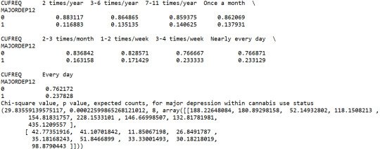
A Chi Square test of independence revealed that among cannabis users aged between 18 and 30 years old (subsetc1), the frequency of cannabis use (explanatory variable collapsed into 9 ordered categories) and past year depression diagnosis (response binary categorical variable) were significantly associated, X2 =29.83, 8 df, p=0.00022.

In the bivariate graph (C->C) presented above, we can see the correlation between frequency of cannabis use (explanatory variable) and major depression diagnosis in the past year (response variable). Obviously, we have a left-skewed distribution, which indicates that the more an individual (18-30) smoked cannabis, the better were the chances to have experienced depression in the last 12 months.

In the first place, for the moderating variable equal to 1, which is those whose a family member or a close friend died in the last 12 months (sub1), a Chi Square test of independence revealed that among cannabis users aged between 18 and 30 years old, the frequency of cannabis use (explanatory variable) and past year depression diagnosis (response variable) were not significantly associated, X2 =4.61, 9 df, p=0.86. As a result, since the chi-square value is quite small and the p-value is significantly large, we can assume that there is no statistical relationship between these two variables, when taking into account the subgroup of individuals who lost a family member or a close friend in the last 12 months.

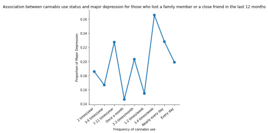
In the bivariate line graph (C->C) presented above, we can see the correlation between frequency of cannabis use (explanatory variable) and major depression diagnosis in the past year (response variable), in the subgroup of individuals whose a family member or a close friend died in the last 12 months (sub1). In fact, the direction of the distribution (fluctuation) does not indicate a positive relationship between these two variables, for those who experienced a family/close death in the past year.

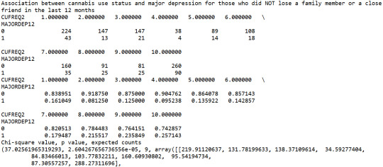
Subsequently, for the moderating variable equal to 2, which is those whose a family member or a close friend did not die in the last 12 months (sub2), a Chi Square test of independence revealed that among cannabis users aged between 18 and 30 years old, the frequency of cannabis use (explanatory variable) and past year depression diagnosis (response variable) were significantly associated, X2 =37.02, 9 df, p=2.6e-05 (p-value is written in scientific notation). As a result, since the chi-square value is quite large and the p-value is significantly small, we can assume that there is a positive relationship between these two variables, when taking into account the subgroup of individuals who did not lose a family member or a close friend in the last 12 months.

In the bivariate line graph (C->C) presented above, we can see the correlation between frequency of cannabis use (explanatory variable) and major depression diagnosis in the past year (response variable), in the subgroup of individuals whose a family member or a close friend did not die in the last 12 months (sub2). Obviously, the direction of the distribution indicates a positive relationship between these two variables, which means that the frequency of cannabis use directly affects the proportions of major depression, regarding the individuals who did not experience a family/close death in the last 12 months.

Summary

It seems that both the direction and the size of the relationship between frequency of cannabis use and major depression diagnosis in the last 12 months, is heavily affected by a death of a family member or a close friend in the same period. In other words, when the incident of a family/close death is present, the correlation is considerably weak, whereas when it is absent, the correlation is significantly strong and positive. Thus, the third variable moderates the association between cannabis use frequency and major depression diagnosis.

0 notes

xaltius · 3 months ago

Text

Common Career Mistakes in Data Science and How to Avoid Them

The field of data science is booming, attracting bright minds eager to unravel insights from the ever-growing ocean of data. However, navigating this exciting career path isn't always smooth sailing. Like any profession, data science has its common pitfalls that can derail progress and hinder success. Whether you're a recent graduate or a seasoned professional transitioning into data science, being aware of these mistakes is the first step towards avoiding them.

1. Focusing Too Much on Tools, Not Enough on Fundamentals:

It's easy to get caught up in learning the latest libraries and frameworks (Python's Pandas, Scikit-learn, TensorFlow, etc.). While tool proficiency is important, neglecting the underlying mathematical and statistical foundations can limit your ability to understand algorithms, interpret results, and solve complex problems effectively.

How to Avoid It: Invest time in strengthening your understanding of linear algebra, calculus, probability, statistics, and machine learning principles. Tools change, but fundamentals remain constant.

2. Jumping Straight into Modeling Without Understanding the Data:

Rushing to build fancy models without thoroughly exploring and understanding the data is a recipe for disaster. This can lead to biased models, inaccurate insights, and ultimately, flawed decisions.

How to Avoid It: Dedicate significant time to exploratory data analysis (EDA). Visualize data, identify patterns, handle missing values, and understand the relationships between variables. This crucial step will inform your modeling choices and lead to more robust results.

3. Ignoring Data Quality:

"Garbage in, garbage out" is a fundamental truth in data science. Working with messy, incomplete, or inaccurate data will inevitably lead to unreliable outcomes.

How to Avoid It: Prioritize data cleaning and preprocessing. Develop skills in identifying and addressing data quality issues. Understand the sources of your data and implement strategies for ensuring its integrity.

4. Building Overly Complex Models:

While sophisticated models can be tempting, simpler models are often more interpretable and robust, especially with limited data. Overly complex models can overfit the training data and perform poorly on unseen data.

How to Avoid It: Start with simpler models and gradually increase complexity only if necessary. Focus on understanding the trade-off between bias and variance. Employ techniques like cross-validation to evaluate model performance on unseen data.

5. Poor Communication and Data Storytelling:

Technical expertise is only half the battle. Data scientists need to effectively communicate their findings to non-technical stakeholders. Failing to translate complex analyses into actionable insights can diminish the impact of your work.

How to Avoid It: Develop strong communication and data visualization skills. Learn to tell compelling stories with data, highlighting the business value of your insights. Practice presenting your work clearly and concisely.

6. Working in Isolation:

Data science is often a collaborative field. Siloed work can lead to missed opportunities, duplicated efforts, and a lack of diverse perspectives.

How to Avoid It: Actively seek collaboration with team members, domain experts, and other stakeholders. Share your work, ask for feedback, and be open to learning from others.

7. Neglecting Domain Knowledge:

Understanding the business context and the domain you're working in is crucial for framing problems effectively and interpreting results accurately.

How to Avoid It: Invest time in learning about the industry, the business processes, and the specific challenges you're trying to address. Collaborate with domain experts to gain valuable insights.

8. Focusing Solely on Accuracy Metrics:

While accuracy is important, it's not the only metric that matters. Depending on the problem, other metrics like precision, recall, F1-score, and AUC might be more relevant.

How to Avoid It: Understand the business implications of different types of errors and choose evaluation metrics that align with your objectives.

9. Not Staying Up-to-Date:

The field of data science is constantly evolving with new algorithms, tools, and best practices emerging regularly. Failing to keep up can quickly make your skills outdated.

How to Avoid It: Dedicate time to continuous learning. Follow industry blogs, attend conferences, take online courses, and engage with the data science community.

10. Underestimating the Importance of Deployment and Production:

Building a great model is only the first step. Getting it into production and ensuring its ongoing performance is critical for delivering business value.

How to Avoid It: Learn about the deployment process, monitoring techniques, and the challenges of maintaining models in a production environment.

Level Up Your Skills with Xaltius Academy's Data Science and AI Course:

While this blog focuses on data science pitfalls, a strong foundation in related areas can significantly enhance your ability to avoid many of them. Xaltius Academy's Data Science and AI Course provides a robust understanding of the core principles and techniques used in the field. This includes machine learning, deep learning, data visualization, and statistical analysis, all essential for becoming a well-rounded and impactful data professional.

Conclusion:

A career in data science offers immense potential, but navigating it successfully requires awareness and proactive effort. By understanding and avoiding these common mistakes, you can steer clear of potential roadblocks and build a fulfilling and impactful career in this exciting field. Remember to focus on fundamentals, understand your data, communicate effectively, and never stop learning.

#artificial intelligence #technology #ai #online course #data science #data science course

1 note · View note

pabloatech · 28 days ago

Text

Week 3:

I put here the script, the results and its description:

PYTHON:

Created on Thu May 22 14:21:21 2025

@author: Pablo """

libraries/packages

import pandas import numpy

read the csv table with pandas:

data = pandas.read_csv('C:/Users/zop2si/Documents/Statistic_tests/nesarc_pds.csv', low_memory=False)

show the dimensions of the data frame:

variables:

variable related to the background of the interviewed people (SES: socioeconomic status):

biological/adopted parents got divorced or stop living together before respondant was 18

data['S1Q2D'] = pandas.to_numeric(data['S1Q2D'], errors='coerce')

variable related to alcohol consumption

HOW OFTEN DRANK ENOUGH TO FEEL INTOXICATED IN LAST 12 MONTHS

data['S2AQ10'] = pandas.to_numeric(data['S2AQ10'], errors='coerce')

variable related to the major depression (low mood I)

EVER HAD 2-WEEK PERIOD WHEN FELT SAD, BLUE, DEPRESSED, OR DOWN MOST OF TIME

data['S4AQ1'] = pandas.to_numeric(data['S4AQ1'], errors='coerce')

Choice of thee variables to display its frequency tables:

string_01 = """ Biological/adopted parents got divorced or stop living together before respondant was 18: 1: yes 2: no 9: unknown -> deleted from the analysis blank: unknown """

string_02 = """ HOW OFTEN DRANK ENOUGH TO FEEL INTOXICATED IN LAST 12 MONTHS

Every day

Nearly every day

3 to 4 times a week

2 times a week

Once a week

2 to 3 times a month

Once a month

7 to 11 times in the last year

3 to 6 times in the last year

1 or 2 times in the last year

Never in the last year

Unknown -> deleted from the analysis BL. NA, former drinker or lifetime abstainer """

string_02b = """ HOW MANY DAYS DRANK ENOUGH TO FEEL INTOXICATED IN THE LAST 12 MONTHS:

"""

string_03 = """ EVER HAD 2-WEEK PERIOD WHEN FELT SAD, BLUE, DEPRESSED, OR DOWN MOST OF TIME:

Yes

Unknown -> deleted from the analysis """

replace unknown values for NaN and remove blanks

data['S1Q2D']=data['S1Q2D'].replace(9, numpy.nan) data['S2AQ10']=data['S2AQ10'].replace(99, numpy.nan) data['S4AQ1']=data['S4AQ1'].replace(9, numpy.nan)

create a subset to know how it works

sub1 = data[['S1Q2D','S2AQ10','S4AQ1']]

create a recode for yearly intoxications:

recode1 = {1:365, 2:313, 3:208, 4:104, 5:52, 6:36, 7:12, 8:11, 9:6, 10:2, 11:0} sub1['Yearly_intoxications'] = sub1['S2AQ10'].map(recode1)

create the tables:

print() c1 = data['S1Q2D'].value_counts(sort=True) # absolute counts

print (c1)

print(string_01) p1 = data['S1Q2D'].value_counts(sort=False, normalize=True) # percentage counts print (p1)

c2 = sub1['Yearly_intoxications'].value_counts(sort=False) # absolute counts

print (c2)

print(string_02b) p2 = sub1['Yearly_intoxications'].value_counts(sort=True, normalize=True) # percentage counts print (p2) print()

c3 = data['S4AQ1'].value_counts(sort=False) # absolute counts

print (c3)

print(string_03) p3 = data['S4AQ1'].value_counts(sort=True, normalize=True) # percentage counts print (p3)

RESULTS:

Biological/adopted parents got divorced or stop living together before respondant was 18: 1: yes 2: no 9: unknown -> deleted from the analysis blank: unknown

2.0 0.814015 1.0 0.185985 Name: S1Q2D, dtype: float64

HOW MANY DAYS DRANK ENOUGH TO FEEL INTOXICATED IN THE LAST 12 MONTHS:

0.0 0.651911 2.0 0.162118 6.0 0.063187 12.0 0.033725 11.0 0.022471 36.0 0.020153 52.0 0.019068 104.0 0.010170 208.0 0.006880 365.0 0.006244 313.0 0.004075 Name: Yearly_intoxications, dtype: float64

EVER HAD 2-WEEK PERIOD WHEN FELT SAD, BLUE, DEPRESSED, OR DOWN MOST OF TIME:

Yes

Unknown -> deleted from the analysis

2.0 0.697045 1.0 0.302955 Name: S4AQ1, dtype: float64

Description:

In regard to computing: the unknown answers were substituted by nan and therefore not considered for the analysis. The original responses to the number of yearly intoxications, which were not a direct figure, were transformed by mapping to yield the actual number of yearly intoxications. For doing this, a submodel was also created.

In regard to the content:

The first variable is quite simple: 18,6% of the respondents saw their parents divorcing before they were 18 years old.

The second variable is the number of yearly intoxications. The highest frequency is as expected not a single intoxication in the last 12 months (65,19%). The more the number of intoxications, the smaller the probability, with an only exception: 0,6% got intoxicated every day and 0,4% got intoxicated almost everyday. I would have expected this numbers flipped.

The last variable points a relatively high frequency of people going through periods of sadness: 30,29%. However, it isn´t yet enough to classify all these periods of sadness as low mood or major depression. A further analysis is necessary.

0 notes

govindhtech · 9 months ago

Text

RAPIDS cuDF Boosts Python Pandas On RTX-powered AI PCs

This article is a part of the AI Decoded series, which shows off new RTX workstation and PC hardware, software, tools, and accelerations while demystifying AI by making the technology more approachable.

AI is fostering innovation and increasing efficiency across sectors, but in order to reach its full potential, the system has to be trained on enormous volumes of high-quality data.

Data scientists are crucial to the preparation of this data, particularly in domain-specific industries where improving AI skills requires specialized, sometimes private data.

NVIDIA revealed that RAPIDS cuDF, a library that makes data manipulation easier for users, speeds up the pandas software library without requiring any code modifications. This is intended to assist data scientists who are facing a growing amount of labor. Pandas is a well-liked, robust, and adaptable Python computer language data analysis and manipulation toolkit. Data scientists may now utilize their favorite code base without sacrificing the speed at which data is processed with RAPIDS cuDF.

Additionally, NVIDIA RTX AI hardware and technology help speed up data processing. Proficient GPUs are among them, providing the computing capacity required to swiftly and effectively boost AI across the board, from data science operations to model training and customization on PCs and workstations.

Python Pandas

Tabular data is the most often used data format; it is arranged in rows and columns. Spreadsheet programs such as Excel may handle smaller datasets; however, modeling pipelines and datasets with tens of millions of rows usually need data frame libraries in Python or other programming languages.

Because of the pandas package, which has an intuitive application programming interface (API), Python is a popular option for data analysis. However, pandas has processing speed and efficiency issues on CPU-only systems as dataset volumes increase. enormous language models need enormous datasets with a lot of text, which the library is infamously bad at handling.

Data scientists are presented with a choice when their data needs exceed pandas’ capabilities: put up with lengthy processing times or make the difficult and expensive decision to migrate to more complicated and expensive technologies that are less user-friendly.

RAPIDS cuDF-Accelerated Preprocessing Pipelines

Data scientists may utilize their favorite code base without compromising processing performance using RAPIDS cuDF.

An open-source collection of the Python packages with GPU acceleration called RAPIDS is intended to enhance data science and analytics workflows. A GPU Data Frame framework called RAPIDS cuDF offers an API for loading, filtering, and modifying data that is similar to pandas.Image credit to Nvidia

Data scientists may take use of strong parallel processing by running their current pandas code on GPUs using RAPIDS cuDF‘s “pandas accelerator mode,” knowing that the code will transition to CPUs as needed. This compatibility offers cutting-edge, dependable performance.

Larger datasets and billions of rows of tabular text data are supported by the most recent version of RAPIDS cuDF. This makes it possible for data scientists to preprocess data for generative AI use cases using pandas code.

NVIDIA RTX-Powered AI Workstations and PCs Improve Data Science

A recent poll indicated that 57% of data scientists use PCs, desktops, or workstations locally.

Significant speedups may be obtained by data scientists beginning with the NVIDIA GeForce RTX 4090 GPU. When compared to conventional CPU-based solutions, cuDF may provide up to 100x greater performance with NVIDIA RTX 6000 Ada Generation GPUs in workstations as datasets expand and processing becomes more memory-intensive.Image credit to Nvidia

With the NVIDIA AI Workbench, data scientists may quickly become proficient with RAPIDS cuDF. Together, data scientists and developers can design, collaborate on, and move AI and data science workloads across GPU systems with our free developer environment manager powered by containers. Several sample projects, like the cuDF AI Workbench project, are available on the NVIDIA GitHub repository to help users get started.

Additionally, cuDF is pre-installed on HP AI Studio, a centralized data science platform intended to assist AI professionals in smoothly migrating their desktop development environment to the cloud. As a result, they may establish, work on projects together, and manage various situations.

Beyond only improving performance, cuDF on RTX-powered AI workstations and PCs has further advantages. It furthermore

Offers fixed-cost local development on strong GPUs that replicates smoothly to on-premises servers or cloud instances, saving time and money.

Enables data scientists to explore, improve, and extract insights from datasets at interactive rates by enabling faster data processing for quicker iterations.

Provides more effective data processing later on in the pipeline for improved model results.

A New Data Science Era

The capacity to handle and analyze large information quickly will become a critical difference as AI and data science continue to advance and allow breakthroughs across sectors. RAPIDS cuDF offers a platform for next-generation data processing, whether it is for creating intricate machine learning models, carrying out intricate statistical analysis, or investigating generative artificial intelligence.

In order to build on this foundation, NVIDIA is supporting the most widely used data frame tools, such as Polaris, one of the fastest-growing Python libraries, which out-of-the-box dramatically speeds up data processing as compared to alternative CPU-only tools.

This month, Polars revealed the availability of the RAPIDS cuDF-powered Polars GPU Engine in open beta. Users of Polars may now increase the already blazingly fast dataframe library’s speed by up to 13 times.