#binarydata
Explore tagged Tumblr posts
Visit Tumblr Blog
Explore Tumblr blogs with no restrictions, modern design and the best experience.
Last Seen Tumblr Blogs


Fun Fact
In February 2021, Tumblr had 518.6 million blog accounts.
Text
What If DNA Could Store All Human Knowledge 2025

What If DNA Could Store All Human Knowledge 2025
Imagine a future where the entire scope of human knowledge — every book, every film, every scientific discovery, and every moment of recorded history — could be encoded and stored inside something as small and essential as a strand of DNA. This idea is no longer purely science fiction. It is based on emerging scientific breakthroughs that combine the powers of biotechnology and information science. So, what would the world look like if DNA could really store all human knowledge? Let’s dive deep into the concept, its implications, and the possibilities it might unlock for the future of information, humanity, and even consciousness itself. Understanding DNA as a Data Storage Medium DNA, the molecule that carries genetic instructions in all living organisms, is incredibly dense when it comes to information storage. Just four nucleotide bases — adenine (A), thymine (T), cytosine (C), and guanine (G) — can be arranged in sequences that represent binary data (0s and 1s), much like the data stored on your phone or computer. In fact, researchers have already successfully encoded images, videos, entire books, and even operating systems into strands of synthetic DNA. For example, in a famous experiment, scientists encoded Shakespeare’s sonnets, an audio file of Martin Luther King Jr.'s “I Have a Dream” speech, and a JPEG image of the Mona Lisa into DNA and retrieved it back with nearly perfect accuracy. The Benefits of Using DNA to Store Human Knowledge Storing data in DNA comes with several major advantages over traditional digital storage systems: - 🧬 Extreme Density: DNA can store up to 215 petabytes (215 million gigabytes) per gram. - 🧬 Longevity: DNA can last for thousands of years if stored in a cool, dry place. Digital hard drives, in contrast, degrade after a few decades. - 🧬 Stability: Unlike magnetic tapes or SSDs that are prone to failure, DNA remains chemically stable for centuries. - 🧬 Universality: DNA is universal, meaning it can be read and copied by any biological system — making it a kind of "future-proof" data format. Now, imagine being able to store the entire internet inside a test tube. This is not a metaphor — it’s a real projection of future possibilities. How Would This Work in Practice? To make DNA storage practical on a global scale, a few technical challenges would need to be solved: - Encoding data into DNA involves converting binary code into sequences of A, T, C, and G. - Synthetic DNA is created using chemical processes that place these sequences in the desired order. - Reading the information back requires sequencing the DNA and decoding it into digital data. At present, this process is expensive and slow. However, rapid advances in biotechnology and AI-driven lab automation are reducing both cost and time. Within a few decades, we could see commercial DNA data storage systems as viable alternatives to cloud storage and hard drives.


Social and Scientific Implications If DNA becomes the ultimate storage device for human knowledge, it could change our society in numerous ways: 1. Revolutionizing Libraries and Archives Physical and digital libraries today consume vast amounts of space, energy, and maintenance. DNA-based libraries would require just a fraction of that space and could survive natural disasters, electromagnetic pulses, or even global internet blackouts. Imagine a tiny capsule carrying every piece of literature, every film, every academic journal — not on a server or in a vault, but in a genetic capsule you could carry in your pocket. 2. Personalized Knowledge Storage People might someday choose to carry personalized knowledge banks encoded in DNA. These could include medical records, learning materials, or even their entire family history. These capsules could be implanted subcutaneously or kept as heirlooms. 3. Integration with Human DNA (A Controversial Twist) The idea of integrating human knowledge directly into a person’s DNA is extremely controversial. But in theory, synthetic sequences could be inserted into non-coding (junk) DNA regions in human cells. This would not impact biological function but could allow for a permanent, inheritable archive of information. While this would raise significant ethical, biological, and privacy concerns, it opens the door to profound possibilities — like transmitting encyclopedic knowledge through generations. Ethical, Legal, and Privacy Concerns This kind of transformative technology doesn’t come without questions: - Who owns the DNA containing human knowledge? - Could it be hacked, corrupted, or stolen? - What if someone stores harmful, illegal, or misleading data? - Should human genomes be used as storage at all? Just like the internet needed laws, standards, and security protocols, DNA data storage will need ethical guidelines and regulatory oversight. Philosophical Questions The concept touches on deep philosophical questions as well: - What is the essence of human knowledge? - If DNA can carry all knowledge, does it bring us closer to a form of digital immortality? - Could one eventually upload parts of their consciousness, memories, or identity using DNA as a carrier? While those questions may remain speculative for now, they are no longer just the musings of science fiction writers — they are becoming real issues that future generations might confront. Potential Drawbacks and Limitations Despite the promise, several barriers still exist: - High Cost: Encoding data into DNA remains expensive and slow. - Read/Write Speeds: Accessing DNA-based data is slower than with digital drives. - Data Mutability: DNA is very stable, but in biological systems, it can mutate. This might be a concern if synthetic DNA interacts with living organisms. However, given the pace of innovation in biotechnology, machine learning, and nanotechnology, these issues may become solvable sooner than we expect. Final Thoughts Storing all human knowledge in DNA is not only feasible — it may become essential. As digital data creation continues to grow exponentially, we’re quickly reaching the physical and economic limits of traditional storage systems. DNA offers a biologically inspired solution with unmatched density, durability, and universality. So, what if DNA could store all human knowledge? The answer might be this: it would change everything — from how we preserve our past to how we shape our future. We would no longer be limited by hard drives or server farms. Instead, we could embed the legacy of humanity into the very fabric of life. And perhaps, one day, a strand of DNA floating in a glass vial could contain the entire story of civilization — all within a few microscopic coils. 📚 Explore our other futuristic topics: - What If Dreams Could Be Recorded and Played Back 2025 https://www.edgythoughts.com/what-if-dreams-could-be-recorded-and-played-back-2025 - What If Humans Could Communicate via Brain-to-Brain Networks 2025 https://www.edgythoughts.com/what-if-humans-could-communicate-via-brain-to-brain-networks-2025 🌐 For more context, visit the Wikipedia page on DNA digital data storage: https://en.wikipedia.org/wiki/DNA_digital_data_storage Read the full article
#1#2#2025-01-01t00:00:00.000+00:00#2025https://www.edgythoughts.com/what-if-dreams-could-be-recorded-and-played-back-2025#2025https://www.edgythoughts.com/what-if-humans-could-communicate-via-brain-to-brain-networks-2025#215#215000000#3#academicjournal#adenine#archive#automation#binarycode#binarydata#biologicalsystem#biotechnology#byte#capsule(fruit)#cell(biology)#chemicalprocess#chemicalsubstance#civilization#cloud#cloudstorage#communicationprotocol#computer#computerdatastorage#concept#consciousness#cost
0 notes
Text
CSV import tutorial shows how to add images or binary data in CSV files for Odoo. Learn efficient methods using XML and Python scripts to process and import image data. #Odoo #CSVImport #Images #BinaryData #Tutorial
0 notes
Text
Website’s Potential with WordPress Hosting
In the digital landscape of today, establishing a strong online presence is paramount, whether you’re launching a personal blog, setting up an e-commerce store, or establishing a professional website for your business. Central to the success of any online venture is the choice of a reliable hosting provider. For those leveraging WordPress as their content management system (CMS), WordPress hosting offers a tailored solution that can significantly enhance your website’s performance, security, and overall user experience.
WHY CHOOSE WORDPRESS HOSTING?
WordPress hosting is tailored specifically for WordPress websites, offering several advantages:
Optimized Performance: Hosting servers are configured to maximize WordPress speed and efficiency, ensuring fast loading times and a seamless user experience.
Enhanced Security: Built-in security features and regular updates protect your site from threats, giving you peace of mind.
Scalability: Easily scale your website as your traffic grows, with options to upgrade resources and accommodate increasing demands.
Simplify Website Management
One of the standout features of Website’s Potential with WordPress Hosting is its ability to simplify website management. Unlike generic web hosting services, WordPress hosting is designed with the unique needs of WordPress users in mind. It includes features such as one-click WordPress installation, automatic updates for WordPress core, themes, and plugins, and intuitive dashboard interfaces that make managing your website straightforward and efficient. This streamlined management process allows you to focus more on creating compelling content and less on technical maintenance.
Enhance Security Measures
Security is a top priority for any website owner, and WordPress hosting excels in this area by offering enhanced security measures tailored specifically for WordPress sites. These may include regular malware scans, proactive threat monitoring, firewalls, and secure authentication protocols. By investing in WordPress hosting, you benefit from a hosting environment that prioritizes the protection of your website and data, ensuring peace of mind for you and a safe browsing experience for your visitors.
Optimize Speed and Performance
Website speed is critical not only for user experience but also for search engine rankings. WordPress hosting providers optimize their servers to ensure fast loading times and optimal performance for WordPress websites. This optimization includes caching mechanisms, content delivery network (CDN) integration, and server-side optimizations that reduce latency and improve response times. A faster website not only enhances user satisfaction but also contributes to higher conversion rates and improved SEO metrics.
KEY FEATURES OF WORDPRESS HOSTING PROVIDER
24/7 Customer Support: Access expert assistance anytime you need it, ensuring your website runs smoothly without interruptions.
One-Click Installation: Effortlessly set up your WordPress site with just a click, saving you time and effort during the initial setup.
Money-Back Guarantee: Enjoy peace of mind with a risk-free trial period, allowing you to test the service without commitment.


EXCLUSIVE DEAL: SAVE 7% ON HOSTINGER HOSTING NOW!
SPECIAL OFFER FOR OUR READERS!
Get Deal
* To host a WordPress-based website, you need to buy WordPress hosting. * For the hosting servers, please use this affiliate link:
*At checkout, use the promo code BINARYDATA to get an additional 7% discount on your total amount.
CONCLUSION
Choosing WordPress hosting for your website or blog is a strategic decision that can significantly impact its success. By opting for WordPress hosting, you gain access to a platform that simplifies management, enhances security, and optimizes performance—all essential elements for a successful online presence.
Whether you’re a blogger, entrepreneur, or small business owner, investing in WordPress hosting is investing in the future of your website. Ready to take your online presence to the next level? Explore the benefits of WordPress hosting and discover how it can help you achieve your goals.
0 notes
Text
Machine Learning for Data Analysis
Week 2: Running a Random Forest
The main drawback to a decision tree is that the tree is highly specific to the dataset it was built on; if you bring in new data to try and predict outcomes, you may not find the same high correlations that your decision tree featured. One method to overcome this is with a random forest. Instead of building one tree from your whole dataset, you subset the data randomly and build a number of trees. Each tree will be different, but the relationships between your variables will tend to appear consistently. In general though, because decision trees are intrinsically connected to the specific data they were built with, decision trees are better as a tool to analyze trends within a known dataset than to create a model for predicting the outcomes of future data.
With those caveats, I decided to build a random forest using the same data as from my previous post, that is, a response variable of internet use rate and explanatory variables of income per person, employment rate, female employment rate, and polity score, from the GapMinder dataset.
Load the data, convert the variables to numeric, convert the response variable to binary, and remove NA values.
In [3]: import pandas as pd import numpy as np import matplotlib.pyplot as plt from sklearn.cross_validation import train_test_split import sklearn.metrics from sklearn.ensemble import ExtraTreesClassifier data = pd.read_csv('c:/users/greg/desktop/gapminder.csv', low_memory=False) data['internetuserate'] = pd.to_numeric(data['internetuserate'], errors='coerce') data['incomeperperson'] = pd.to_numeric(data['incomeperperson'], errors='coerce') data['employrate'] = pd.to_numeric(data['employrate'], errors='coerce') data['femaleemployrate'] = pd.to_numeric(data['femaleemployrate'], errors='coerce') data['polityscore'] = pd.to_numeric(data['polityscore'], errors='coerce') binarydata = data.copy() # convert response variable to binarydef internetgrp (row): if row['internetuserate'] < data['internetuserate'].median(): return 0 else: return 1 binarydata['internetuserate'] = binarydata.apply (lambda row: internetgrp (row),axis=1) # Clean the dataset binarydata_clean = binarydata.dropna()
Build the model from the training set
In [10]:predictors = binarydata_clean[['incomeperperson','employrate','femaleemployrate','polityscore']] targets = binarydata_clean.internetuserate pred_train, pred_test, tar_train, tar_test = train_test_split(predictors, targets, test_size=.4) from sklearn.ensemble import RandomForestClassifier classifier_r=RandomForestClassifier(n_estimators=25) classifier_r=classifier_r.fit(pred_train,tar_train) predictions_r=classifier_r.predict(pred_test)
Print the confusion matrix
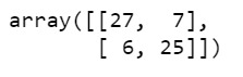
In [11]:sklearn.metrics.confusion_matrix(tar_test,predictions_r)
Out[11]:array([[22, 5], [10, 24]])
Print the accuracy score
In [12]:sklearn.metrics.accuracy_score(tar_test, predictions_r)
Out[12]:0.75409836065573765
Fit an Extra Trees model to the data
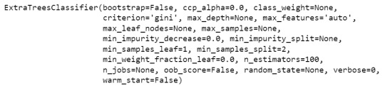
In [13]:model_r = ExtraTreesClassifier() model_r.fit(pred_train,tar_train)
Out[13]:ExtraTreesClassifier(bootstrap=False, class_weight=None, criterion='gini', max_depth=None, max_features='auto', max_leaf_nodes=None, min_samples_leaf=1, min_samples_split=2, min_weight_fraction_leaf=0.0, n_estimators=10, n_jobs=1, oob_score=False, random_state=None, verbose=0, warm_start=False)
Display the Relative Importances of Each Attribute
In [15]:model_r.feature_importances_
Out[15]:array([ 0.44072852, 0.12553198, 0.1665162 , 0.2672233 ])
Run a different number of trees and see the effect of that on the accuracy of the prediction
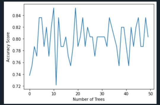
In [16]:trees=range(50) accuracy=np.zeros(50) for idx in range(len(trees)): classifier_r=RandomForestClassifier(n_estimators=idx + 1) classifier_r=classifier_r.fit(pred_train,tar_train) predictions_r=classifier_r.predict(pred_test) accuracy[idx]=sklearn.metrics.accuracy_score(tar_test, predictions_r) plt.cla() plt.plot(trees, accuracy) plt.ylabel('Accuracy Score') plt.xlabel('Number of Trees') plt.show()

The confusion matrix and accuracy score are similar to that of my previous post (remember, a decision tree is pseudo-randomly created, so results will be similar, but not identical, when run with the same dataset). Examining the relative importance of each attribute is interesting here. As expected, income per person is the most highly correlated with internet use rate, at 54% of the model’s predictive capability. Employment rate (15%) and female employment rate (11%) are less correlated, again, as expected. But polity score, at 20% of the model’s predictive capability, stood out to me because none of the previous models I’ve examined with this dataset have had polity score even near the same level of importance as employment rates. Interesting. Finally, the graph shows that as the number of trees in the forest grows, the accuracy of the model does as well, but only up to about 20 trees. After that, the accuracy stops increasing and instead fluctuates with the random permutations of the subsets of data that were used to create the trees.
0 notes
Text
Coursera- Machine Learning - Week 2 Assignment
The main drawback to a decision tree is that the tree is highly specific to the dataset it was built on; if you bring in new data to try and predict outcomes, you may not find the same high correlations that your decision tree featured. One method to overcome this is with a random forest. Instead of building one tree from your whole dataset, you subset the data randomly and build a number of trees. Each tree will be different, but the relationships between your variables will tend to appear consistently. In general though, because decision trees are intrinsically connected to the specific data they were built with, decision trees are better as a tool to analyze trends within a known dataset than to create a model for predicting the outcomes of future data.
Code:
import pandas as pd import numpy as np import matplotlib.pyplot as plt from sklearn.model_selection import train_test_split import sklearn.metrics from sklearn.ensemble import ExtraTreesClassifier
data = pd.read_csv(r'C:\Users\AL58114\Downloads\gapminder.csv', low_memory=False)
data['internetuserate'] = pd.to_numeric(data['internetuserate'], errors='coerce') data['incomeperperson'] = pd.to_numeric(data['incomeperperson'], errors='coerce') data['employrate'] = pd.to_numeric(data['employrate'], errors='coerce') data['femaleemployrate'] = pd.to_numeric(data['femaleemployrate'], errors='coerce') data['polityscore'] = pd.to_numeric(data['polityscore'], errors='coerce')
binarydata = data.copy()
#convert response variable to binary
def internetgrp (row): if row['internetuserate'] < data['internetuserate'].median(): return 0 else: return 1
binarydata['internetuserate'] = binarydata.apply (lambda row: internetgrp (row),axis=1)
#Clean the dataset
binarydata_clean = binarydata.dropna()
predictors = binarydata_clean[['incomeperperson','employrate','femaleemployrate','polityscore']] targets = binarydata_clean.internetuserate pred_train, pred_test, tar_train, tar_test = train_test_split(predictors, targets, test_size=.4)
from sklearn.ensemble import RandomForestClassifier
classifier_r=RandomForestClassifier(n_estimators=25) classifier_r=classifier_r.fit(pred_train,tar_train) predictions_r=classifier_r.predict(pred_test)
#Print the confusion matrix
sklearn.metrics.confusion_matrix(tar_test,predictions_r)
#Print the accuracy score
sklearn.metrics.accuracy_score(tar_test, predictions_r)
#Fit an Extra Trees model to the data
model_r = ExtraTreesClassifier() model_r.fit(pred_train,tar_train)
#Display the Relative Importances of Each Attribute
model_r.feature_importances_
#Run a different number of trees and see the accuracy of the prediction
trees=range(50) accuracy=np.zeros(50)
for idx in range(len(trees)): classifier_r=RandomForestClassifier(n_estimators=idx + 1) classifier_r=classifier_r.fit(pred_train,tar_train) predictions_r=classifier_r.predict(pred_test) accuracy[idx]=sklearn.metrics.accuracy_score(tar_test, predictions_r)
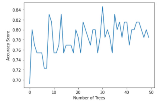
plt.cla() plt.plot(trees, accuracy) plt.ylabel('Accuracy Score') plt.xlabel('Number of Trees') plt.show()
Results:
Interpretation:
The confusion matrix and accuracy score are similar to that of my previous post. Examining the relative importance of each attribute is interesting here. As expected, income per person is the most highly correlated with internet use rate, at 54% of the model’s predictive capability. Employment rate (15%) and female employment rate (11%) are less correlated, again, as expected. But polity score, at 20% of the model’s predictive capability, stood out to me because none of the previous models I’ve examined with this dataset have had polity score even near the same level of importance as employment rates. Interesting. Finally, the graph shows that as the number of trees in the forest grows, the accuracy of the model does as well, but only up to about 20 trees. After that, the accuracy stops increasing and instead fluctuates with the random permutations of the subsets of data that were used to create the trees.
0 notes
Text
Machine Learning for Data Analysis - Week 2
#Load the data and convert the variables to numeric
import pandas as pd import numpy as np import matplotlib.pyplot as plt from sklearn.model_selection import train_test_split import sklearn.metrics from sklearn.ensemble import ExtraTreesClassifier
data = pd.read_csv('gapminder.csv', low_memory=False)
data['urbanrate'] = pd.to_numeric(data['urbanrate'], errors='coerce') data['incomeperperson'] = pd.to_numeric(data['incomeperperson'], errors='coerce') data['femaleemployrate'] = pd.to_numeric(data['femaleemployrate'], errors='coerce') data['breastcancerper100th'] = pd.to_numeric(data['breastcancerper100th'], errors='coerce')
binarydata = data.copy()
#convert response variable to binary
def internetgrp (row): if row['urbanrate'] < data['urbanrate'].median(): return 0 else: return 1
binarydata['urbanrate'] = binarydata.apply (lambda row: internetgrp (row),axis=1)
#Clean the dataset
binarydata_clean = binarydata.dropna()
predictors = binarydata_clean[['incomeperperson','femaleemployrate','breastcancerper100th']] targets = binarydata_clean.urbanrate pred_train, pred_test, tar_train, tar_test = train_test_split(predictors, targets, test_size=.4)
from sklearn.ensemble import RandomForestClassifier
classifier_r=RandomForestClassifier(n_estimators=25) classifier_r=classifier_r.fit(pred_train,tar_train) predictions_r=classifier_r.predict(pred_test)
#Print the confusion matrix
sklearn.metrics.confusion_matrix(tar_test,predictions_r)
#Print the accuracy score
sklearn.metrics.accuracy_score(tar_test, predictions_r)

#Fit an Extra Trees model to the data
model_r = ExtraTreesClassifier() model_r.fit(pred_train,tar_train)
#Display the Relative Importances of Each Attribute
model_r.feature_importances_

#Run a different number of trees and see the effect of that on the accuracy of the prediction
trees=range(50) accuracy=np.zeros(50)
for idx in range(len(trees)): classifier_r=RandomForestClassifier(n_estimators=idx + 1) classifier_r=classifier_r.fit(pred_train,tar_train) predictions_r=classifier_r.predict(pred_test) accuracy[idx]=sklearn.metrics.accuracy_score(tar_test, predictions_r)
plt.cla() plt.plot(trees, accuracy) plt.ylabel('Accuracy Score') plt.xlabel('Number of Trees') plt.show()
0 notes
Photo

Best Ios App Development Company Mohali | Binary Data Pvt Ltd Binary Data Pvt Ltd is the best ios app development company in Mohali, India. This platform offers many features and functionalities in the fields of apps or games and also this platform focused on the user experience. We are the specialized team of ios app developers who will work on backend development of an application with clean code. Contact us Email:[email protected] Website:-https://www.binarydata.in
#Binary Data Pvt Ltd#Best Ios App Development Company Mohali#best ios app development company#mobile app development services#mobile app development services india#ios app development software services#binarydata#best it company#best web design and web development company#best it company india
1 note
·
View note
Photo

Best App Development Company Halifax, Canada
Binary Data is one of the best app development company Halifax, Toronto, Brampton, Burlington, Hamilton, Kitchener. Our expert Android app developers are focused to provide integrated and user-engaging mobile apps. Professionals at Binary Data develop your Apps with fresh and crisp ideas.
#Best App Development Company Halifax Canada#App Development Company#binarydata#App developers halifax#mobile app development halifax#app development company halifax#halifax app development#app development halifax#mobile app development company halifax
0 notes
Photo

#WebDevelopment#ResponsiveWebDesign#MockUp#PSD#BootStrap#Wordpress#Joomla#Magento#php#websitedevelopment#binarydata#Itservices#websitedesigning
0 notes
Text
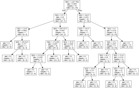
Machine Learning for Data Analysis Week 1: Running a Classification Tree For the next few posts, I’ll be exploring machine learning techniques to help analyze the Gap Minder data. To begin, I’ll create a classification tree to explore the relationship between my response variable, internet user rate, and my explanatory variables, income per person, employment rate, female employment rate, and polity score. The technique requires a binary, categorical response variable, so for the purpose of this demonstration I have binned internet use rate into two categories, High usage and Low usage, split by the median data point. Load the data and convert the variables to numeric In [1]: ''' Code for Peer-graded Assignments: Running a Classification Tree Course: Data Management and Visualization Specialization: Data Analysis and Interpretation ''' import pandas as pd from sklearn.cross_validation import train_test_split from sklearn.tree import DecisionTreeClassifier import sklearn.metrics data = pd.read_csv('c:/users/greg/desktop/gapminder.csv', low_memory=False) data['internetuserate'] = pd.to_numeric(data['internetuserate'], errors='coerce') data['incomeperperson'] = pd.to_numeric(data['incomeperperson'], errors='coerce') data['employrate'] = pd.to_numeric(data['employrate'], errors='coerce') data['femaleemployrate'] = pd.to_numeric(data['femaleemployrate'], errors='coerce') data['polityscore'] = pd.to_numeric(data['polityscore'], errors='coerce') Convert the response variable to binary In [3]: binarydata = data.copy() def internetgrp (row): if row['internetuserate'] < data['internetuserate'].median(): return 0 else: return 1 binarydata['internetuserate'] = binarydata.apply (lambda row: internetgrp (row),axis=1) Clean the data by discarding NA values In [4]: binarydata_clean = binarydata.dropna() binarydata_clean.dtypes binarydata_clean.describe() Out[4]: incomeperperson femaleemployrate internetuserate polityscore employrate count 152.000000 152.000000 152.000000 152.000000 152.000000 mean 6706.556978 48.068421 0.453947 3.861842 59.212500 std 9823.592315 14.826857 0.499521 6.245581 10.363802 min 103.775857 12.400000 0.000000 -10.000000 34.900002 25% 560.797158 39.549999 0.000000 -2.000000 51.924999 50% 2225.931019 48.549999 0.000000 7.000000 58.900002 75% 6905.287662 56.050000 1.000000 9.000000 65.000000 max 39972.352768 83.300003 1.000000 10.000000 83.199997 Split into training and testing sets In [7]: predictors = binarydata_clean[['incomeperperson','employrate','femaleemployrate','polityscore']] targets = binarydata_clean.internetuserate pred_train, pred_test, tar_train, tar_test = train_test_split(predictors, targets, test_size=.4) print ('Training sample') print (pred_train.shape) print ('') print ('Testing sample') print (pred_test.shape) print ('') print ('Training sample') print (tar_train.shape) print ('') print ('Testing sample') print (tar_test.shape) Training sample (91, 4) Testing sample (61, 4) Training sample (91,) Testing sample (61,) Build model on the training data In [8]: classifier=DecisionTreeClassifier() classifier=classifier.fit(pred_train,tar_train) predictions=classifier.predict(pred_test) Display the confusion matrix In [10]: sklearn.metrics.confusion_matrix(tar_test,predictions) Out[10]: array([[22, 9], [ 8, 22]]) Display the accuracy score In [11]: sklearn.metrics.accuracy_score(tar_test, predictions) Out[11]: 0.72131147540983609 Display the decision tree In [13]: from sklearn import tree from io import StringIO from IPython.display import Image out = StringIO() tree.export_graphviz(classifier, out_file=out) import pydotplus graph=pydotplus.graph_from_dot_data(out.getvalue()) Image(graph.create_png()) Out[13]: The decision tree analysis was performed to test non-linear relationships among the explanatory variables and a single binary, categorical response variable. The training sample has 91 rows of data and 4 explanatory variables; the testing sample has 61 rows of data, and the same 4 explanatory variables. The decision tree results in 27 true negatives and 16 true positives; and 11 false negatives and 7 false positives. The accuracy score is 70.5%, meaning that the model accurately predicted 70.5% of the internet use rates per country.
1 note
·
View note
Text
RUNNING A RANDOM FOREST
The main drawback to a decision tree is that the tree is highly specific to the dataset it was built on; if you bring in new data to try and predict outcomes, you may not find the same high correlations that your decision tree featured. One method to overcome this is with a random forest. Instead of building one tree from your whole dataset, you subset the data randomly and build a number of trees. Each tree will be different, but the relationships between your variables will tend to appear consistently. In general though, because decision trees are intrinsically connected to the specific data they were built with, decision trees are better as a tool to analyze trends within a known dataset than to create a model for predicting the outcomes of future data.
With those caveats, I decided to build a random forest using the same data as from my previous post, that is, a response variable of internet use rate and explanatory variables of income per person, employment rate, female employment rate, and polity score, from the GapMinder dataset.
Load the data, convert the variables to numeric, convert the response variable to binary, and remove NA values.
In [3]:''' Code for Peer-graded Assignments: Running a Random Forest Course: Data Management and Visualization Specialization: Data Analysis and Interpretation ''' import pandas as pd import numpy as np import matplotlib.pyplot as plt from sklearn.cross_validation import train_test_split import sklearn.metrics from sklearn.ensemble import ExtraTreesClassifier data = pd.read_csv('c:/users/greg/desktop/gapminder.csv', low_memory=False) data['internetuserate'] = pd.to_numeric(data['internetuserate'], errors='coerce') data['incomeperperson'] = pd.to_numeric(data['incomeperperson'], errors='coerce') data['employrate'] = pd.to_numeric(data['employrate'], errors='coerce') data['femaleemployrate'] = pd.to_numeric(data['femaleemployrate'], errors='coerce') data['polityscore'] = pd.to_numeric(data['polityscore'], errors='coerce') binarydata = data.copy() # convert response variable to binarydef internetgrp (row): if row['internetuserate'] < data['internetuserate'].median(): return 0 else: return 1 binarydata['internetuserate'] = binarydata.apply (lambda row: internetgrp (row),axis=1) # Clean the dataset binarydata_clean = binarydata.dropna()
Build the model from the training set
In [10]:predictors = binarydata_clean[['incomeperperson','employrate','femaleemployrate','polityscore']] targets = binarydata_clean.internetuserate pred_train, pred_test, tar_train, tar_test = train_test_split(predictors, targets, test_size=.4) from sklearn.ensemble import RandomForestClassifier classifier_r=RandomForestClassifier(n_estimators=25) classifier_r=classifier_r.fit(pred_train,tar_train) predictions_r=classifier_r.predict(pred_test)
Print the confusion matrix
In [11]:sklearn.metrics.confusion_matrix(tar_test,predictions_r)
Out[11]:array([[22, 5], [10, 24]])
Print the accuracy score
In [12]:sklearn.metrics.accuracy_score(tar_test, predictions_r)
Out[12]:0.75409836065573765
Fit an Extra Trees model to the data
In [13]:model_r = ExtraTreesClassifier() model_r.fit(pred_train,tar_train)
Out[13]:ExtraTreesClassifier(bootstrap=False, class_weight=None, criterion='gini', max_depth=None, max_features='auto', max_leaf_nodes=None, min_samples_leaf=1, min_samples_split=2, min_weight_fraction_leaf=0.0, n_estimators=10, n_jobs=1, oob_score=False, random_state=None, verbose=0, warm_start=False)
Display the Relative Importances of Each Attribute
In [15]:model_r.feature_importances_
Out[15]:array([ 0.44072852, 0.12553198, 0.1665162 , 0.2672233 ])
Run a different number of trees and see the effect of that on the accuracy of the prediction
In [16]:trees=range(50) accuracy=np.zeros(50) for idx in range(len(trees)): classifier_r=RandomForestClassifier(n_estimators=idx + 1) classifier_r=classifier_r.fit(pred_train,tar_train) predictions_r=classifier_r.predict(pred_test) accuracy[idx]=sklearn.metrics.accuracy_score(tar_test, predictions_r) plt.cla() plt.plot(trees, accuracy) plt.ylabel('Accuracy Score') plt.xlabel('Number of Trees') plt.show()

64.media.tumblr.com
The confusion matrix and accuracy score are similar to that of my previous post (remember, a decision tree is pseudo-randomly created, so results will be similar, but not identical, when run with the same dataset). Examining the relative importance of each attribute is interesting here. As expected, income per person is the most highly correlated with internet use rate, at 54% of the model’s predictive capability. Employment rate (15%) and female employment rate (11%) are less correlated, again, as expected. But polity score, at 20% of the model’s predictive capability, stood out to me because none of the previous models I’ve examined with this dataset have had polity score even near the same level of importance as employment rates. Interesting. Finally, the graph shows that as the number of trees in the forest grows, the accuracy of the model does as well, but only up to about 20 trees. After that, the accuracy stops increasing and instead fluctuates with the random permutations of the subsets of data that were used to create the trees.
More from @chidujs
chidujsFollow
machine learning week1
For the next few posts, I’ll be exploring machine learning techniques to help analyze the GapMinder data. To begin, I’ll create a classification tree to explore the relationship between my response variable, internet user rate, and my explanatory variables, income per person, employment rate, female employment rate, and polity score. The technique requires a binary, categorical response variable, so for the purpose of this demonstration I have binned internet use rate into two categories, High usage and Low usage, split by the median data point.
Load the data and convert the variables to numeric
In [1]:''' Code for Peer-graded Assignments: Running a Classification Tree Course: Data Management and Visualization Specialization: Data Analysis and Interpretation ''' import pandas as pd from sklearn.cross_validation import train_test_split from sklearn.tree import DecisionTreeClassifier import sklearn.metrics data = pd.read_csv('c:/users/greg/desktop/gapminder.csv', low_memory=False) data['internetuserate'] = pd.to_numeric(data['internetuserate'], errors='coerce') data['incomeperperson'] = pd.to_numeric(data['incomeperperson'], errors='coerce') data['employrate'] = pd.to_numeric(data['employrate'], errors='coerce') data['femaleemployrate'] = pd.to_numeric(data['femaleemployrate'], errors='coerce') data['polityscore'] = pd.to_numeric(data['polityscore'], errors='coerce')
Convert the response variable to binary
In [3]:binarydata = data.copy() def internetgrp (row): if row['internetuserate'] < data['internetuserate'].median(): return 0 else: return 1 binarydata['internetuserate'] = binarydata.apply (lambda row: internetgrp (row),axis=1)
Clean the data by discarding NA values
In [4]:binarydata_clean = binarydata.dropna() binarydata_clean.dtypes binarydata_clean.describe()
Out[4]:incomeperpersonfemaleemployrateinternetuseratepolityscoreemployratecount152.000000152.000000152.000000152.000000152.000000mean6706.55697848.0684210.4539473.86184259.212500std9823.59231514.8268570.4995216.24558110.363802min103.77585712.4000000.000000-10.00000034.90000225%560.79715839.5499990.000000-2.00000051.92499950%2225.93101948.5499990.0000007.00000058.90000275%6905.28766256.0500001.0000009.00000065.000000max39972.35276883.3000031.00000010.00000083.199997
Split into training and testing sets
In [7]:predictors = binarydata_clean[['incomeperperson','employrate','femaleemployrate','polityscore']] targets = binarydata_clean.internetuserate pred_train, pred_test, tar_train, tar_test = train_test_split(predictors, targets, test_size=.4) print ('Training sample') print (pred_train.shape) print ('') print ('Testing sample') print (pred_test.shape) print ('') print ('Training sample') print (tar_train.shape) print ('') print ('Testing sample') print (tar_test.shape) Training sample (91, 4) Testing sample (61, 4) Training sample (91,) Testing sample (61,)
Build model on the training data
In [8]:classifier=DecisionTreeClassifier() classifier=classifier.fit(pred_train,tar_train) predictions=classifier.predict(pred_test)
Display the confusion matrix
In [10]:sklearn.metrics.confusion_matrix(tar_test,predictions)
Out[10]:array([[22, 9], [ 8, 22]])
Display the accuracy score
In [11]:sklearn.metrics.accuracy_score(tar_test, predictions)
Out[11]:0.72131147540983609
Display the decision tree
In [13]:from sklearn import tree from io import StringIO from IPython.display import Image out = StringIO() tree.export_graphviz(classifier, out_file=out) import pydotplus graph=pydotplus.graph_from_dot_data(out.getvalue()) Image(graph.create_png())
Out[13]:
64.media.tumblr.com
The decision tree analysis was performed to test non-linear relationships among the explanatory variables and a single binary, categorical response variable. The training sample has 91 rows of data and 4 explanatory variables; the testing sample has 61 rows of data, and the same 4 explanatory variables. The decision tree results in 27 true negatives and 16 true positives; and 11 false negatives and 7 false positives. The accuracy score is 70.5%, meaning that the model accurately predicted 70.5% of the internet use rates per country.
chidujsFollow
THE GAPMINDER data
Sample
I am using the GapMinder dataset to investigate the relationship between internet usage in a country and that country’s GDP, overall employment rate, female employment rate, and its “polity score”, which is a measure of a country’s democratic and free nature. The sample contains data on a country-level for 215 regions (the 192 U.N. countries, with Serbia and Montenegro aggregated into one, as well as 24 other non-country regions, such as Monaco for instance). The study population is these 215 countries and regions and my sample data is the same; ie, the population is small enough that no sample is necessary to make the data collecting and processing more manageable.
Procedure
The data has been collected by the non-profit venture GapMinder from a handful of sources, including the Institute for Health Metrics and Evaluation, the US Census Bureau’s International Database, the United Nations Statistics Division, and the World Bank. In the case of each data collection organization, data was collected from detailed surveys of the country’s population (such as in a national census) and based mainly upon 2010 data. Employment rate data comes from 2007 and polity score from 2009. Polity score is calculated by subtracting the autocracy score from the democracy score from the Polity IV project’s research. GapMinder’s goal in collecting this data is to help world leaders and their citizens to better understand the forces shaping the geopolitical landscape around the globe.
Measures
My response variable is the internet use rate and my explanatory variables are income per person, employment rate, female employment rate, and polity score. Internet use rate, employment rate, and female employment rate are scaled as percentages of the country’s population. Income per person is simply Gross Domestic Product per capita (the country’s total, country-wide income divided by the population). Polity score is a single measure applied to the whole country. The internet use rate of a country was collected by the World Bank in their World Development Indicators. Income per person is simply the 2010 Gross Domestic Product per capita in constant 2000 USD. The inflation, but not the differences in the cost of living between countries, has been taken into account (this can lead to the seemingly odd case of a having negative income per person, when that country already has very low income relative to the United States plus high inflation, relative to the United States). Both employment rate and female employment rate have been provided by the International Labour Organization. Finally, the polity score has been calculated by the Polity IV project.
I have gone through the data and removed entries where data is missing, when necessary, and sometimes have aggregated data into bins, for histograms, for instance, but otherwise have not modified the data in any way. Deeper data management was unnecessary for the analysis.
chidujsFollow
Logistic Regression Model
import numpy
import pandas
import statsmodels.api as sm
import seaborn
import statsmodels.formula.api as smf
# bug fix for display formats to avoid run time errorspandas.set_option('display.float_format', lambda x:'%.2f'%x)nesarc = pandas.read_csv ('nesarc_pds.csv' , low_memory=False)
#Set PANDAS to show all columns in DataFramepandas.set_option('display.max_columns', None)
#Set PANDAS to show all rows in DataFramepandas.set_option('display.max_rows', None) nesarc.columns = map(str.upper , nesarc.columns)
# Change my variables to numeric nesarc['S3BQ1A5'] = pandas.to_numeric(nesarc['S3BQ1A5'], errors='coerce')nesarc['MARP12ABDEP'] = pandas.to_numeric(nesarc['MARP12ABDEP'], errors='coerce') # Cannabis abuse/dependencenesarc['COCP12ABDEP'] = pandas.to_numeric(nesarc['COCP12ABDEP'], errors='coerce') # Cocaine abuse/dependencenesarc['ALCABDEPP12DX'] = pandas.to_numeric(nesarc['ALCABDEPP12DX'], errors='coerce') # Alcohol abuse/dependencenesarc['HERP12ABDEP'] = pandas.to_numeric(nesarc['HERP12ABDEP'], errors='coerce')
# Heroin abuse/dependencenesarc['MAJORDEP12'] = pandas.to_numeric(nesarc['MAJORDEP12'], errors='coerce')
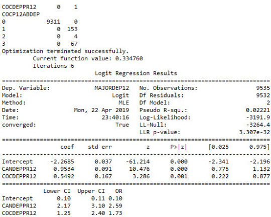
# Major depression # Subset my sample: ages 18-30 sub1=nesarc[(nesarc['AGE']>=18) & (nesarc['AGE']<=30)] ############################################################################### LOGISTIC REGRESSION############################################################################## # Binary cannabis abuse/dependence prior to the last 12 months def CANDEPPR12 (x1): if x1['MARP12ABDEP']==1 or x1['MARP12ABDEP']==2 or x1['MARP12ABDEP']==3: return 1 else: return 0sub1['CANDEPPR12'] = sub1.apply (lambda x1: CANDEPPR12 (x1), axis=1)print (pandas.crosstab(sub1['MARP12ABDEP'], sub1['CANDEPPR12'])) ## Logistic regression with cannabis abuse/dependence (explanatory) - major depression (response) logreg1 = smf.logit(formula = 'MAJORDEP12 ~ CANDEPPR12', data = sub1).fit()print (logreg1.summary())# odds ratiosprint ("Odds Ratios")print (numpy.exp(logreg1.params))
# Odd ratios with 95% confidence intervals params = logreg1.paramsconf = logreg1.conf_int()conf['OR'] = paramsconf.columns = ['Lower CI', 'Upper CI', 'OR']print (numpy.exp(conf))
# Binary cocaine abuse/dependence prior to the last 12 months def COCDEPPR12 (x2): if x2['COCP12ABDEP']==1 or x2['COCP12ABDEP']==2 or x2['COCP12ABDEP']==3: return 1 else: return 0sub1['COCDEPPR12'] = sub1.apply (lambda x2: COCDEPPR12 (x2), axis=1)print (pandas.crosstab(sub1['COCP12ABDEP'], sub1['COCDEPPR12']))
## Logistic regression with cannabis and cocaine abuse/depndence (explanatory) - major depression (response) logreg2 = smf.logit(formula = 'MAJORDEP12 ~ CANDEPPR12 + COCDEPPR12', data = sub1).fit()print (logreg2.summary()) # Odd ratios with 95% confidence intervals params = logreg2.paramsconf = logreg2.conf_int()conf['OR'] = paramsconf.columns = ['Lower CI', 'Upper CI', 'OR']print (numpy.exp(conf))
# Binary alcohol abuse/dependence prior to the last 12 months def ALCDEPPR12 (x2): if x2['ALCABDEPP12DX']==1 or x2['ALCABDEPP12DX']==2 or x2['ALCABDEPP12DX']==3: return 1 else: return 0sub1['ALCDEPPR12'] = sub1.apply (lambda x2: ALCDEPPR12 (x2), axis=1)print (pandas.crosstab(sub1['ALCABDEPP12DX'], sub1['ALCDEPPR12']))
# Binary sedative abuse/dependence prior to the last 12 months def HERDEPPR12 (x3): if x3['HERP12ABDEP']==1 or x3['HERP12ABDEP']==2 or x3['HERP12ABDEP']==3: return 1 else: return 0sub1['HERDEPPR12'] = sub1.apply (lambda x3: HERDEPPR12 (x3), axis=1)print (pandas.crosstab(sub1['HERP12ABDEP'], sub1['HERDEPPR12']))
## Logistic regression with alcohol abuse/depndence (explanatory) - major depression (response) logreg3 = smf.logit(formula = 'MAJORDEP12 ~ HERDEPPR12', data = sub1).fit()print (logreg3.summary()) # Odd ratios with 95% confidence intervals print ("Odds Ratios")params = logreg3.paramsconf = logreg3.conf_int()conf['OR'] = paramsconf.columns = ['Lower CI', 'Upper CI', 'OR']print (numpy.exp(conf))
## Logistic regression with cannabis and alcohol abuse/depndence (explanatory) - major depression (response) logreg4 = smf.logit(formula = 'MAJORDEP12 ~ CANDEPPR12 + ALCDEPPR12 + COCDEPPR12', data = sub1).fit()print (logreg4.summary()) # Odd ratios with 95% confidence intervals print ("Odds Ratios")params = logreg4.paramsconf = logreg4.conf_int()conf['OR'] = paramsconf.columns = ['Lower CI', 'Upper CI', 'OR']print (numpy.exp(conf))
result:
64.media.tumblr.com

64.media.tumblr.com
chidujsFollow
Multiple Regression Model
import numpy
import pandas
import statsmodels.api as sm
import seaborn
import statsmodels.formula.api as smf
import matplotlib.pyplot as plt
# bug fix for display formats to avoid run time errorspandas.set_option('display.float_format', lambda x:'%.2f'%x)nesarc = pandas.read_csv ('nesarc_pds.csv' , low_memory=False)
#Set PANDAS to show all columns in DataFramepandas.set_option('display.max_columns', None)#Set PANDAS to show all rows in DataFramepandas.set_option('display.max_rows', None) nesarc.columns = map(str.upper , nesarc.columns) # Change my variables to numeric nesarc['IDNUM'] =pandas.to_numeric(nesarc['IDNUM'], errors='coerce')nesarc['S3BQ1A5'] = pandas.to_numeric(nesarc['S3BQ1A5'], errors='coerce')nesarc['MAJORDEP12'] = pandas.to_numeric(nesarc['MAJORDEP12'], errors='coerce') # Major depressionnesarc['AGE'] =pandas.to_numeric(nesarc['AGE'], errors='coerce')nesarc['SEX'] = pandas.to_numeric(nesarc['SEX'], errors='coerce')nesarc['S3BD5Q2E'] = pandas.to_numeric(nesarc['S3BD5Q2E'], errors='coerce') # Cannabis use frequencynesarc['S3BQ4'] = pandas.to_numeric(nesarc['S3BQ4'], errors='coerce') # Quantity of joints per daynesarc['GENAXDX12'] = pandas.to_numeric(nesarc['GENAXDX12'], errors='coerce') # General anxietynesarc['S3BD5Q2F'] = pandas.to_numeric(nesarc['S3BD5Q2F'], errors='coerce') # Age when began using cannabis the mostnesarc['DYSDX12'] = pandas.to_numeric(nesarc['DYSDX12'], errors='coerce')
# Dysthymianesarc['SOCPDX12'] = pandas.to_numeric(nesarc['SOCPDX12'], errors='coerce') # Social phobianesarc['S3BD5Q2GR'] = pandas.to_numeric(nesarc['S3BD5Q2GR'], errors='coerce') # Cannabis use duration (weeks)nesarc['S3CD5Q15C'] = pandas.to_numeric(nesarc['S3CD5Q15C'], errors='coerce') # Cannabis dependencenesarc['S3CD5Q13B'] = pandas.to_numeric(nesarc['S3CD5Q13B'], errors='coerce')
# Cannabis abuse # Current cannabis abuse criterianesarc['S3CD5Q14C9'] = pandas.to_numeric(nesarc['S3CD5Q14C9'], errors='coerce')nesarc['S3CQ14A8'] = pandas.to_numeric(nesarc['S3CQ14A8'], errors='coerce') # Longer period cannabis abuse criterianesarc['S3CD5Q14C3'] = pandas.to_numeric(nesarc['S3CD5Q14C3'], errors='coerce') # Depressed because of cannabis effects wearing offnesarc['S3CD5Q14C6C'] = pandas.to_numeric(nesarc['S3CD5Q14C6C'], errors='coerce') # Sleep difficulties because of cannabis effects wearing offnesarc['S3CD5Q14C6R'] = pandas.to_numeric(nesarc['S3CD5Q14C6R'], errors='coerce')
# Eat more because of cannabis effects wearing offnesarc['S3CD5Q14C6H'] = pandas.to_numeric(nesarc['S3CD5Q14C6H'], errors='coerce') # Feel nervous or anxious because of cannabis effects wearing offnesarc['S3CD5Q14C6I'] = pandas.to_numeric(nesarc['S3CD5Q14C6I'], errors='coerce')
# Fast heart beat because of cannabis effects wearing offnesarc['S3CD5Q14C6D'] = pandas.to_numeric(nesarc['S3CD5Q14C6D'], errors='coerce') # Feel weak or tired because of cannabis effects wearing offnesarc['S3CD5Q14C6B'] = pandas.to_numeric(nesarc['S3CD5Q14C6B'], errors='coerce')
# Withdrawal symptomsnesarc['S3CD5Q14C6U'] = pandas.to_numeric(nesarc['S3CD5Q14C6U'], errors='coerce')
# Subset my sample: Cannabis users, ages 18-30 sub1=nesarc[(nesarc['AGE']>=18) & (nesarc['AGE']<=30) & (nesarc['S3BQ1A5']==1)] ###############
Cannabis abuse/dependence criteria in the last 12 months (response variable) ############### #
Current cannabis abuse/dependence criteria #1 DSM-IV def crit1 (row): if row['S3CD5Q14C9']==1 or row['S3CQ14A8'] == 1 : return 1 elif row['S3CD5Q14C9']==2 and row['S3CQ14A8']==2 : return 0sub1['crit1'] = sub1.apply (lambda row: crit1 (row),axis=1) # Current 6 cannabis abuse/dependence sub-symptoms criteria #2 DSM-IV # Recode for summing (from 1,2 to 0,1)recode1 = {1: 1, 2: 0}sub1['S3CD5Q14C6C']=sub1['S3CD5Q14C6C'].replace(9, numpy.nan)sub1['S3CD5Q14C6C']= sub1['S3CD5Q14C6C'].map(recode1)sub1['S3CD5Q14C6R']=sub1['S3CD5Q14C6R'].replace(9, numpy.nan)sub1['S3CD5Q14C6R']= sub1['S3CD5Q14C6R'].map(recode1)sub1['S3CD5Q14C6H']=sub1['S3CD5Q14C6H'].replace(9, numpy.nan)sub1['S3CD5Q14C6H']= sub1['S3CD5Q14C6H'].map(recode1)sub1['S3CD5Q14C6I']=sub1['S3CD5Q14C6I'].replace(9, numpy.nan)sub1['S3CD5Q14C6I']= sub1['S3CD5Q14C6I'].map(recode1)sub1['S3CD5Q14C6D']=sub1['S3CD5Q14C6D'].replace(9, numpy.nan)sub1['S3CD5Q14C6D']= sub1['S3CD5Q14C6D'].map(recode1)sub1['S3CD5Q14C6B']=sub1['S3CD5Q14C6B'].replace(9, numpy.nan)sub1['S3CD5Q14C6B']= sub1['S3CD5Q14C6B'].map(recode1)
# Sum symptomssub1['CWITHDR_COUNT'] = numpy.nansum([sub1['S3CD5Q14C6C'], sub1['S3CD5Q14C6R'], sub1['S3CD5Q14C6H'], sub1['S3CD5Q14C6I'], sub1['S3CD5Q14C6D'], sub1['S3CD5Q14C6B']], axis=0) # Sum code checkchksum=sub1[['IDNUM','S3CD5Q14C6C', 'S3CD5Q14C6R', 'S3CD5Q14C6H', 'S3CD5Q14C6I', 'S3CD5Q14C6D', 'S3CD5Q14C6B', 'CWITHDR_COUNT']]chksum.head(n=50)
# Withdrawal symptoms in the last 12 months (yes/no)def crit2 (row): if row['CWITHDR_COUNT']>=3 or row['S3CD5Q14C6U']==1: return 1 elif row['CWITHDR_COUNT']<3 and row['S3CD5Q14C6U']!=1: return 0sub1['crit2'] = sub1.apply (lambda row: crit2 (row),axis=1) # Longer period cannabis abuse/dependence criteria #3 DSM-IV sub1['S3CD5Q14C3']=sub1['S3CD5Q14C3'].replace(9, numpy.nan)sub1['S3CD5Q14C3']= sub1['S3CD5Q14C3'].map(recode1)
# Current cannabis use cut down criteria #4 DSM-IV sub1['S3CD5Q14C2'] = pandas.to_numeric(sub1['S3CD5Q14C2'], errors='coerce') # Without successsub1['S3CD5Q14C1'] = pandas.to_numeric(sub1['S3CD5Q14C1'], errors='coerce') # More than oncedef crit4 (row): if row['S3CD5Q14C2']==1 or row['S3CD5Q14C1'] == 1 : return 1 elif row['S3CD5Q14C2']==2 and row['S3CD5Q14C1']==2 : return 0sub1['crit4'] = sub1.apply (lambda row: crit4 (row),axis=1)chk1e = sub1['crit4'].value_counts(sort=False, dropna=False)
# Current reduce of important/pleasurable activities criteria #5 DSM-IV sub1['S3CD5Q14C10'] = pandas.to_numeric(sub1['S3CD5Q14C10'], errors='coerce')sub1['S3CD5Q14C11'] = pandas.to_numeric(sub1['S3CD5Q14C11'], errors='coerce')def crit5 (row): if row['S3CD5Q14C10']==1 or row['S3CD5Q14C11'] == 1 : return 1 elif row['S3CD5Q14C10']==2 and row['S3CD5Q14C11']==2 : return 0sub1['crit5'] = sub1.apply (lambda row: crit5 (row),axis=1)chk1g = sub1['crit5'].value_counts(sort=False, dropna=False) # Current cannbis use continuation despite knowledge of physical or psychological problem criteria
#6 DSM-IV sub1['S3CD5Q14C13'] = pandas.to_numeric(sub1['S3CD5Q14C13'], errors='coerce')sub1['S3CD5Q14C12'] = pandas.to_numeric(sub1['S3CD5Q14C12'], errors='coerce')def crit6 (row): if row['S3CD5Q14C13']==1 or row['S3CD5Q14C12'] == 1 : return 1 elif row['S3CD5Q14C13']==2 and row['S3CD5Q14C12']==2 : return 0sub1['crit6'] = sub1.apply (lambda row: crit6 (row),axis=1)chk1h = sub1['crit6'].value_counts(sort=False, dropna=False)
# Cannabis abuse/dependence symptoms sum sub1['CanDepSymptoms'] = numpy.nansum([sub1['crit1'], sub1['crit2'], sub1['S3CD5Q14C3'], sub1['crit4'], sub1['crit5'], sub1['crit6']], axis=0 )chk2 = sub1['CanDepSymptoms'].value_counts(sort=False, dropna=False) ############################################################################### MULTIPLE REGRESSION & CONFIDENCE INTERVALS
############################################################################## sub2 = sub1[['S3BQ4', 'S3BD5Q2F', 'DYSDX12', 'MAJORDEP12', 'CanDepSymptoms', 'SOCPDX12', 'GENAXDX12', 'S3BD5Q2GR']].dropna()
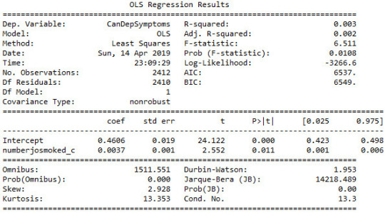
# Centre the quantity of joints smoked per day and age when they began using cannabis, quantitative variablessub1['numberjosmoked_c'] = (sub1['S3BQ4'] - sub1['S3BQ4'].mean())sub1['agebeganuse_c'] = (sub1['S3BD5Q2F'] - sub1['S3BD5Q2F'].mean())sub1['canuseduration_c'] = (sub1['S3BD5Q2GR'] - sub1['S3BD5Q2GR'].mean()) # Linear regression analysis print('OLS regression model for the association between major depression diagnosis and cannabis depndence symptoms')reg1 = smf.ols('CanDepSymptoms ~ MAJORDEP12', data=sub1).fit()print (reg1.summary()) print('OLS regression model for the association of majord depression diagnosis and smoking quantity with cannabis dependence symptoms')reg2 = smf.ols('CanDepSymptoms ~ MAJORDEP12 + DYSDX12', data=sub1).fit()print (reg2.summary()) reg3 = smf.ols('CanDepSymptoms ~ MAJORDEP12 + agebeganuse_c + numberjosmoked_c + canuseduration_c + GENAXDX12 + DYSDX12 + SOCPDX12', data=sub1).fit()print (reg3.summary())
##################################################################################### POLYNOMIAL REGRESSION
#################################################################################### #
First order (linear) scatterplotscat1 = seaborn.regplot(x="S3BQ4", y="CanDepSymptoms", scatter=True, data=sub1)plt.ylim(0, 6)plt.xlabel('Quantity of joints')plt.ylabel('Cannabis dependence symptoms') # Fit second order polynomialscat1 = seaborn.regplot(x="S3BQ4", y="CanDepSymptoms", scatter=True, order=2, data=sub1)plt.ylim(0, 6)plt.xlabel('Quantity of joints')plt.ylabel('Cannabis dependence symptoms') # Linear regression analysisreg4 = smf.ols('CanDepSymptoms ~ numberjosmoked_c', data=sub1).fit()print (reg4.summary()) reg5 = smf.ols('CanDepSymptoms ~ numberjosmoked_c + I(numberjosmoked_c**2)',
data=sub1).fit()print (reg5.summary()) ##################################################################################### EVALUATING MODEL FIT
####################################################################################
recode1 = {1: 10, 2: 9, 3: 8, 4: 7, 5: 6, 6: 5, 7: 4, 8: 3, 9: 2, 10: 1} # Dictionary with details of frequency variable reverse-recodesub1['CUFREQ'] = sub1['S3BD5Q2E'].map(recode1) # Change variable name from S3BD5Q2E to CUFREQ sub1['CUFREQ_c'] = (sub1['CUFREQ'] - sub1['CUFREQ'].mean()) # Adding frequency of cannabis usereg6 = smf.ols('CanDepSymptoms ~ numberjosmoked_c + I(numberjosmoked_c**2) + CUFREQ_c', data=sub1).fit()print (reg6.summary()) # Q-Q plot for normalityfig1=sm.qqplot(reg6.resid, line='r')print (fig1)
# Simple plot of residualsstdres=pandas.DataFrame(reg6.resid_pearson)fig2=plt.plot(stdres, 'o', ls='None')l = plt.axhline(y=0, color='r')plt.ylabel('Standardized Residual')plt.xlabel('Observation Number') # Additional regression diagnostic plotsfig3 = plt.figure(figsize=(12,8))fig3 = sm.graphics.plot_regress_exog(reg6, "CUFREQ_c", fig=fig3) # leverage plotfig4 = plt.figure(figsize=(36,24))fig4=sm.graphics.influence_plot(reg6, size=2)print(fig4)
OUTPUT:
64.media.tumblr.com

64.media.tumblr.com
chidujsFollow
BASIC REGRESSION MODEL
import numpy
import pandas
import statsmodels.api as sm
import seaborn
import statsmodels.formula.api as smf
import matplotlib.pyplot as plt
# bug fix for display formats to avoid run time errorspandas.set_option('display.float_format', lambda x:'%.2f'%x) nesarc = pandas.read_csv ('nesarc_pds.csv' , low_memory=False) #Set PANDAS to show all columns in DataFramepandas.set_option('display.max_columns', None)#Set PANDAS to show all rows in DataFramepandas.set_option('display.max_rows', None) nesarc.columns = map(str.upper , nesarc.columns) # Change my variables to numeric nesarc['IDNUM'] =pandas.to_numeric(nesarc['IDNUM'], errors='coerce')nesarc['S3BQ1A5'] = pandas.to_numeric(nesarc['S3BQ1A5'], errors='coerce')nesarc['MAJORDEP12'] = pandas.to_numeric(nesarc['MAJORDEP12'], errors='coerce')nesarc['AGE'] =pandas.to_numeric(nesarc['AGE'], errors='coerce')nesarc['SEX'] = pandas.to_numeric(nesarc['SEX'], errors='coerce')nesarc['S3BD5Q2E'] = pandas.to_numeric(nesarc['S3BD5Q2E'], errors='coerce') # Current cannabis abuse criterianesarc['S3CD5Q14C9'] = pandas.to_numeric(nesarc['S3CD5Q14C9'], errors='coerce')nesarc['S3CQ14A8'] = pandas.to_numeric(nesarc['S3CQ14A8'], errors='coerce') # Longer period cannabis abuse criterianesarc['S3CD5Q14C3'] = pandas.to_numeric(nesarc['S3CD5Q14C3'], errors='coerce') # Depressed because of cannabis effects wearing offnesarc['S3CD5Q14C6C'] = pandas.to_numeric(nesarc['S3CD5Q14C6C'], errors='coerce') # Sleep difficulties because of cannabis effects wearing offnesarc['S3CD5Q14C6R'] = pandas.to_numeric(nesarc['S3CD5Q14C6R'], errors='coerce') # Eat more because of cannabis effects wearing offnesarc['S3CD5Q14C6H'] = pandas.to_numeric(nesarc['S3CD5Q14C6H'], errors='coerce') # Feel nervous or anxious because of cannabis effects wearing offnesarc['S3CD5Q14C6I'] = pandas.to_numeric(nesarc['S3CD5Q14C6I'], errors='coerce') # Fast heart beat because of cannabis effects wearing offnesarc['S3CD5Q14C6D'] = pandas.to_numeric(nesarc['S3CD5Q14C6D'], errors='coerce') # Feel weak or tired because of cannabis effects wearing offnesarc['S3CD5Q14C6B'] = pandas.to_numeric(nesarc['S3CD5Q14C6B'], errors='coerce') # Withdrawal symptomsnesarc['S3CD5Q14C6U'] = pandas.to_numeric(nesarc['S3CD5Q14C6U'], errors='coerce') # Subset my sample: Cannabis users, ages 18-30 sub1=nesarc[(nesarc['AGE']>=18) & (nesarc['AGE']<=30) & (nesarc['S3BQ1A5']==1)] (pandas.crosstab(sub1['S3CD5Q14C9'], sub1['S3CQ14A8'])) c1 = sub1['S3CD5Q14C6U'].value_counts(sort=False, dropna=False)print (c1) # Current 6 cannabis abuse/dependence sub-symptoms criteria #2 DSM-IV # Recode for summing (from 1,2 to 0,1)recode1 = {1: 1, 2: 0}sub1['S3CD5Q14C6C']=sub1['S3CD5Q14C6C'].replace(9, numpy.nan)sub1['S3CD5Q14C6C']= sub1['S3CD5Q14C6C'].map(recode1)sub1['S3CD5Q14C6R']=sub1['S3CD5Q14C6R'].replace(9, numpy.nan)sub1['S3CD5Q14C6R']= sub1['S3CD5Q14C6R'].map(recode1)sub1['S3CD5Q14C6H']=sub1['S3CD5Q14C6H'].replace(9, numpy.nan)sub1['S3CD5Q14C6H']= sub1['S3CD5Q14C6H'].map(recode1)sub1['S3CD5Q14C6I']=sub1['S3CD5Q14C6I'].replace(9, numpy.nan)sub1['S3CD5Q14C6I']= sub1['S3CD5Q14C6I'].map(recode1)sub1['S3CD5Q14C6D']=sub1['S3CD5Q14C6D'].replace(9, numpy.nan)sub1['S3CD5Q14C6D']= sub1['S3CD5Q14C6D'].map(recode1)sub1['S3CD5Q14C6B']=sub1['S3CD5Q14C6B'].replace(9, numpy.nan)sub1['S3CD5Q14C6B']= sub1['S3CD5Q14C6B'].map(recode1) # Check recodechk1c = sub1['S3CD5Q14C6U'].value_counts(sort=False, dropna=False)print (chk1c) # Sum symptomssub1['CWITHDR_COUNT'] = numpy.nansum([sub1['S3CD5Q14C6C'], sub1['S3CD5Q14C6R'], sub1['S3CD5Q14C6H'], sub1['S3CD5Q14C6I'], sub1['S3CD5Q14C6D'], sub1['S3CD5Q14C6B']], axis=0) # Sum code checkchksum=sub1[['IDNUM','S3CD5Q14C6C', 'S3CD5Q14C6R', 'S3CD5Q14C6H', 'S3CD5Q14C6I', 'S3CD5Q14C6D', 'S3CD5Q14C6B', 'CWITHDR_COUNT']]chksum.head(n=50) chk1d = sub1['CWITHDR_COUNT'].value_counts(sort=False, dropna=False)print (chk1d)
# Withdrawal symptoms in the last 12 months (yes/no)def crit2 (row): if row['CWITHDR_COUNT']>=3 or row['S3CD5Q14C6U']==1: return 1 elif row['CWITHDR_COUNT']<3 and row['S3CD5Q14C6U']!=1: return 0sub1['crit2'] = sub1.apply (lambda row: crit2 (row),axis=1)print (pandas.crosstab(sub1['CWITHDR_COUNT'], sub1['crit2'])) # Longer period cannabis abuse/dependence criteria #3 DSM-IV sub1['S3CD5Q14C3']=sub1['S3CD5Q14C3'].replace(9, numpy.nan)sub1['S3CD5Q14C3']= sub1['S3CD5Q14C3'].map(recode1) chk1d = sub1['S3CD5Q14C3'].value_counts(sort=False, dropna=False)print (chk1d) # Current cannabis use cut down criteria #4 DSM-IV sub1['S3CD5Q14C2'] = pandas.to_numeric(sub1['S3CD5Q14C2'], errors='coerce') # Without successsub1['S3CD5Q14C1'] = pandas.to_numeric(sub1['S3CD5Q14C1'], errors='coerce') # More than oncedef crit4 (row): if row['S3CD5Q14C2']==1 or row['S3CD5Q14C1'] == 1 : return 1 elif row['S3CD5Q14C2']==2 and row['S3CD5Q14C1']==2 : return 0sub1['crit4'] = sub1.apply (lambda row: crit4 (row),axis=1)chk1e = sub1['crit4'].value_counts(sort=False, dropna=False)print (chk1e) # Current reduce of important/pleasurable activities criteria
#5 DSM-IV sub1['S3CD5Q14C10'] = pandas.to_numeric(sub1['S3CD5Q14C10'], errors='coerce')sub1['S3CD5Q14C11'] = pandas.to_numeric(sub1['S3CD5Q14C11'], errors='coerce')def crit5 (row): if row['S3CD5Q14C10']==1 or row['S3CD5Q14C11'] == 1 : return 1 elif row['S3CD5Q14C10']==2 and row['S3CD5Q14C11']==2 : return 0sub1['crit5'] = sub1.apply (lambda row: crit5 (row),axis=1)chk1g = sub1['crit5'].value_counts(sort=False, dropna=False)print (chk1g) # Current cannbis use continuation despite knowledge of physical or psychological problem criteria #6 DSM-IV sub1['S3CD5Q14C13'] = pandas.to_numeric(sub1['S3CD5Q14C13'], errors='coerce')sub1['S3CD5Q14C12'] = pandas.to_numeric(sub1['S3CD5Q14C12'], errors='coerce')def crit6 (row): if row['S3CD5Q14C13']==1 or row['S3CD5Q14C12'] == 1 : return 1 elif row['S3CD5Q14C13']==2 and row['S3CD5Q14C12']==2 : return 0sub1['crit6'] = sub1.apply (lambda row: crit6 (row),axis=1)chk1h = sub1['crit6'].value_counts(sort=False, dropna=False)print (chk1h) # Cannabis abuse/dependence symptoms sum sub1['CanDepSymptoms'] = numpy.nansum([sub1['crit1'], sub1['crit2'], sub1['S3CD5Q14C3'], sub1['crit4'], sub1['crit5'], sub1['crit6']], axis=0 )
chk2 = sub1['CanDepSymptoms'].value_counts(sort=False, dropna=False)
print (chk2) c1 = sub1["MAJORDEP12"].value_counts(sort=False, dropna=False)print(c1)c2 = sub1["AGE"].value_counts(sort=False, dropna=False)print(c2)
############### Major depression diagnosis in the last 12 months (explanatory variable) ############### # Major depression diagnosis print('OLS regression model for the association between major depression diagnosis and cannabis depndence symptoms')reg1 = smf.ols('CanDepSymptoms ~ MAJORDEP12', data=sub1).fit()print (reg1.summary()) # Listwise deletion for calculating means for regression model observations sub1 = sub1[['CanDepSymptoms', 'MAJORDEP12']].dropna() # Group means & sd print ("Mean")ds1 = sub1.groupby('MAJORDEP12').mean()print (ds1)print ("Standard deviation")ds2 = sub1.groupby('MAJORDEP12').std()print (ds2) # Bivariate bar graph print('Bivariate bar graph for major depression diagnosis and cannabis depndence symptoms')
seaborn.factorplot(x="MAJORDEP12", y="CanDepSymptoms", data=sub1, kind="bar", ci=None)plt.xlabel('Major Depression Diagnosis')plt.ylabel('Mean Number of Cannabis Dependence Symptoms')

64.media.tumblr.com
chidujsFollow
writing about your data assignment
Sample
I am using the GapMinder dataset to investigate the relationship between internet usage in a country and that country’s GDP, overall employment rate, female employment rate, and its “polity score”, which is a measure of a country’s democratic and free nature. The sample contains data on a country-level for 215 regions (the 192 U.N. countries, with Serbia and Montenegro aggregated into one, as well as 24 other non-country regions, such as Monaco for instance). The study population is these 215 countries and regions and my sample data is the same; ie, the population is small enough that no sample is necessary to make the data collecting and processing more manageable.
Procedure
The data has been collected by the non-profit venture GapMinder from a handful of sources, including the Institute for Health Metrics and Evaluation, the US Census Bureau’s International Database, the United Nations Statistics Division, and the World Bank. In the case of each data collection organization, data was collected from detailed surveys of the country’s population (such as in a national census) and based mainly upon 2010 data. Employment rate data comes from 2007 and polity score from 2009. Polity score is calculated by subtracting the autocracy score from the democracy score from the Polity IV project’s research. GapMinder’s goal in collecting this data is to help world leaders and their citizens to better understand the forces shaping the geopolitical landscape around the globe.
Measures
My response variable is the internet use rate and my explanatory variables are income per person, employment rate, female employment rate, and polity score. Internet use rate, employment rate, and female employment rate are scaled as percentages of the country’s population. Income per person is simply Gross Domestic Product per capita (the country’s total, country-wide income divided by the population). Polity score is a single measure applied to the whole country. The internet use rate of a country was collected by the World Bank in their World Development Indicators. Income per person is simply the 2010 Gross Domestic Product per capita in constant 2000 USD. The inflation, but not the differences in the cost of living between countries, has been taken into account (this can lead to the seemingly odd case of a having negative income per person, when that country already has very low income relative to the United States plus high inflation, relative to the United States). Both employment rate and female employment rate have been provided by the International Labour Organization. Finally, the polity score has been calculated by the Polity IV project.
I have gone through the data and removed entries where data is missing, when necessary, and sometimes have aggregated data into bins, for histograms, for instance, but otherwise have not modified the data in any way.Deeper data management was unnecessary for the analysis.
chidujsFollow
Assignment.
@@ -0,0 +1,157 @@
-- coding: utf-8 --
""" Created on Sun Mar 17 18:11:22 2019 @author: Voltas """ import pandas import numpy import seaborn import scipy import matplotlib.pyplot as plt
nesarc = pandas.read_csv ('nesarc_pds.csv', low_memory=False)
Set PANDAS to show all columns in DataFrame
pandas.set_option('display.max_columns' , None)
Set PANDAS to show all rows in DataFrame
pandas.set_option('display.max_rows' , None)
nesarc.columns = map(str.upper , nesarc.columns)
pandas.set_option('display.float_format' , lambda x:'%f'%x)
Change my variables to numeric
nesarc['AGE'] = nesarc['AGE'].convert_objects(convert_numeric=True) nesarc['MAJORDEP12'] = nesarc['MAJORDEP12'].convert_objects(convert_numeric=True) nesarc['S1Q231'] = nesarc['S1Q231'].convert_objects(convert_numeric=True) nesarc['S3BQ1A5'] = nesarc['S3BQ1A5'].convert_objects(convert_numeric=True) nesarc['S3BD5Q2E'] = nesarc['S3BD5Q2E'].convert_objects(convert_numeric=True)
Subset my sample
subset1 = nesarc[(nesarc['AGE']>=18) & (nesarc['AGE']<=30) & nesarc['S3BQ1A5']==1] # Ages 18-30, cannabis users subsetc1 = subset1.copy()
Setting missing data
subsetc1['S1Q231']=subsetc1['S1Q231'].replace(9, numpy.nan) subsetc1['S3BQ1A5']=subsetc1['S3BQ1A5'].replace(9, numpy.nan) subsetc1['S3BD5Q2E']=subsetc1['S3BD5Q2E'].replace(99, numpy.nan) subsetc1['S3BD5Q2E']=subsetc1['S3BD5Q2E'].replace('BL', numpy.nan) recode1 = {1: 9, 2: 8, 3: 7, 4: 6, 5: 5, 6: 4, 7: 3, 8: 2, 9: 1} # Frequency of cannabis use variable reverse-recode subsetc1['CUFREQ'] = subsetc1['S3BD5Q2E'].map(recode1) # Change the variable name from S3BD5Q2E to CUFREQ
subsetc1['CUFREQ'] = subsetc1['CUFREQ'].astype('category')
Raname graph labels for better interpetation
subsetc1['CUFREQ'] = subsetc1['CUFREQ'].cat.rename_categories(["2 times/year","3-6 times/year","7-11 times/year","Once a month","2-3 times/month","1-2 times/week","3-4 times/week","Nearly every day","Every day"])
Contingency table of observed counts of major depression diagnosis (response variable) within frequency of cannabis use groups (explanatory variable), in ages 18-30
contab1 = pandas.crosstab(subsetc1['MAJORDEP12'], subsetc1['CUFREQ']) print (contab1)
Column percentages
colsum=contab1.sum(axis=0) colpcontab=contab1/colsum print(colpcontab)
Chi-square calculations for major depression within frequency of cannabis use groups
print ('Chi-square value, p value, expected counts, for major depression within cannabis use status') chsq1= scipy.stats.chi2_contingency(contab1) print (chsq1)
Bivariate bar graph for major depression percentages with each cannabis smoking frequency group
plt.figure(figsize=(12,4)) # Change plot size ax1 = seaborn.factorplot(x="CUFREQ", y="MAJORDEP12", data=subsetc1, kind="bar", ci=None) ax1.set_xticklabels(rotation=40, ha="right") # X-axis labels rotation plt.xlabel('Frequency of cannabis use') plt.ylabel('Proportion of Major Depression') plt.show()
recode2 = {1: 10, 2: 9, 3: 8, 4: 7, 5: 6, 6: 5, 7: 4, 8: 3, 9: 2, 10: 1} # Frequency of cannabis use variable reverse-recode subsetc1['CUFREQ2'] = subsetc1['S3BD5Q2E'].map(recode2) # Change the variable name from S3BD5Q2E to CUFREQ2
sub1=subsetc1[(subsetc1['S1Q231']== 1)] sub2=subsetc1[(subsetc1['S1Q231']== 2)]
print ('Association between cannabis use status and major depression for those who lost a family member or a close friend in the last 12 months') contab2=pandas.crosstab(sub1['MAJORDEP12'], sub1['CUFREQ2']) print (contab2)
Column percentages
colsum2=contab2.sum(axis=0) colpcontab2=contab2/colsum2 print(colpcontab2)
Chi-square
print ('Chi-square value, p value, expected counts') chsq2= scipy.stats.chi2_contingency(contab2) print (chsq2)
Line graph for major depression percentages within each frequency group, for those who lost a family member or a close friend
plt.figure(figsize=(12,4)) # Change plot size ax2 = seaborn.factorplot(x="CUFREQ", y="MAJORDEP12", data=sub1, kind="point", ci=None) ax2.set_xticklabels(rotation=40, ha="right") # X-axis labels rotation plt.xlabel('Frequency of cannabis use') plt.ylabel('Proportion of Major Depression') plt.title('Association between cannabis use status and major depression for those who lost a family member or a close friend in the last 12 months') plt.show()
#
print ('Association between cannabis use status and major depression for those who did NOT lose a family member or a close friend in the last 12 months') contab3=pandas.crosstab(sub2['MAJORDEP12'], sub2['CUFREQ2']) print (contab3)
Column percentages
colsum3=contab3.sum(axis=0) colpcontab3=contab3/colsum3 print(colpcontab3)
Chi-square
print ('Chi-square value, p value, expected counts') chsq3= scipy.stats.chi2_contingency(contab3) print (chsq3)
Line graph for major depression percentages within each frequency group, for those who did NOT lose a family member or a close friend
plt.figure(figsize=(12,4)) # Change plot size ax3 = seaborn.factorplot(x="CUFREQ", y="MAJORDEP12", data=sub2, kind="point", ci=None) ax3.set_xticklabels(rotation=40, ha="right") # X-axis labels rotation plt.xlabel('Frequency of cannabis use') plt.ylabel('Proportion of Major Depression') plt.title('Association between cannabis use status and major depression for those who did NOT lose a family member or a close friend in the last 12 months') plt.show()
chidujsFollow
Assignment3
@@ -0,0 +1,97 @@
-- coding: utf-8 --
""" Created on Thu Mar 7 15:00:39 2019 @author: Voltas """
import pandas import numpy import seaborn import scipy import matplotlib.pyplot as plt
nesarc = pandas.read_csv ('nesarc_pds.csv' , low_memory=False)
Set PANDAS to show all columns in DataFrame
pandas.set_option('display.max_columns', None)
Set PANDAS to show all rows in DataFrame
pandas.set_option('display.max_rows', None) nesarc.columns = map(str.upper , nesarc.columns)
pandas.set_option('display.float_format' , lambda x:'%f'%x)
Change my variables to numeric
nesarc['AGE'] = pandas.to_numeric(nesarc['AGE'], errors='coerce') nesarc['S3BQ4'] = pandas.to_numeric(nesarc['S3BQ4'], errors='coerce') nesarc['S4AQ6A'] = pandas.to_numeric(nesarc['S4AQ6A'], errors='coerce') nesarc['S3BD5Q2F'] = pandas.to_numeric(nesarc['S3BD5Q2F'], errors='coerce') nesarc['S9Q6A'] = pandas.to_numeric(nesarc['S9Q6A'], errors='coerce') nesarc['S4AQ7'] = pandas.to_numeric(nesarc['S4AQ7'], errors='coerce') nesarc['S3BQ1A5'] = pandas.to_numeric(nesarc['S3BQ1A5'], errors='coerce')
Subset my sample
subset1 = nesarc[(nesarc['S3BQ1A5']==1)] # Cannabis users subsetc1 = subset1.copy()
Setting missing data
subsetc1['S3BQ1A5']=subsetc1['S3BQ1A5'].replace(9, numpy.nan) subsetc1['S3BD5Q2F']=subsetc1['S3BD5Q2F'].replace('BL', numpy.nan) subsetc1['S3BD5Q2F']=subsetc1['S3BD5Q2F'].replace(99, numpy.nan) subsetc1['S4AQ6A']=subsetc1['S4AQ6A'].replace('BL', numpy.nan) subsetc1['S4AQ6A']=subsetc1['S4AQ6A'].replace(99, numpy.nan) subsetc1['S9Q6A']=subsetc1['S9Q6A'].replace('BL', numpy.nan) subsetc1['S9Q6A']=subsetc1['S9Q6A'].replace(99, numpy.nan)
Scatterplot for the age when began using cannabis the most and the age of first episode of major depression
plt.figure(figsize=(12,4)) # Change plot size scat1 = seaborn.regplot(x="S3BD5Q2F", y="S4AQ6A", fit_reg=True, data=subset1) plt.xlabel('Age when began using cannabis the most') plt.ylabel('Age when expirenced the first episode of major depression') plt.title('Scatterplot for the age when began using cannabis the most and the age of first the episode of major depression') plt.show()
data_clean=subset1.dropna()
Pearson correlation coefficient for the age when began using cannabis the most and the age of first the episode of major depression
print ('Association between the age when began using cannabis the most and the age of the first episode of major depression') print (scipy.stats.pearsonr(data_clean['S3BD5Q2F'], data_clean['S4AQ6A']))
Scatterplot for the age when began using cannabis the most and the age of the first episode of general anxiety
plt.figure(figsize=(12,4)) # Change plot size scat2 = seaborn.regplot(x="S3BD5Q2F", y="S9Q6A", fit_reg=True, data=subset1) plt.xlabel('Age when began using cannabis the most') plt.ylabel('Age when expirenced the first episode of general anxiety') plt.title('Scatterplot for the age when began using cannabis the most and the age of the first episode of general anxiety') plt.show()
Pearson correlation coefficient for the age when began using cannabis the most and the age of the first episode of general anxiety
print ('Association between the age when began using cannabis the most and the age of first the episode of general anxiety') print (scipy.stats.pearsonr(data_clean['S3BD5Q2F'], data_clean['S9Q6A']))
chidujsFollow
ASSIGNMENT
-- coding: utf-8 --
""" Created on Fri Mar 1 17:20:15 2019 @author: Voltas """
import pandas import numpy import scipy.stats import seaborn import matplotlib.pyplot as plt
nesarc = pandas.read_csv ('nesarc_pds.csv' , low_memory=False)
Set PANDAS to show all columns in DataFrame
pandas.set_option('display.max_columns', None)
Set PANDAS to show all rows in DataFrame
pandas.set_option('display.max_rows', None)
nesarc.columns = map(str.upper , nesarc.columns)
pandas.set_option('display.float_format' , lambda x:'%f'%x)
Change my variables to numeric
nesarc['AGE'] = pandas.to_numeric(nesarc['AGE'], errors='coerce') nesarc['S3BQ4'] = pandas.to_numeric(nesarc['S3BQ4'], errors='coerce') nesarc['S3BQ1A5'] = pandas.to_numeric(nesarc['S3BQ1A5'], errors='coerce') nesarc['S3BD5Q2B'] = pandas.to_numeric(nesarc['S3BD5Q2B'], errors='coerce') nesarc['S3BD5Q2E'] = pandas.to_numeric(nesarc['S3BD5Q2E'], errors='coerce') nesarc['MAJORDEP12'] = pandas.to_numeric(nesarc['MAJORDEP12'], errors='coerce') nesarc['GENAXDX12'] = pandas.to_numeric(nesarc['GENAXDX12'], errors='coerce')
Subset my sample
subset1 = nesarc[(nesarc['AGE']>=18) & (nesarc['AGE']<=30)] # Ages 18-30 subsetc1 = subset1.copy()
subset2 = nesarc[(nesarc['AGE']>=18) & (nesarc['AGE']<=30) & (nesarc['S3BQ1A5']==1)] # Cannabis users, ages 18-30 subsetc2 = subset2.copy()
Setting missing data for frequency and cannabis use, variables S3BD5Q2E, S3BQ1A5
subsetc1['S3BQ1A5']=subsetc1['S3BQ1A5'].replace(9, numpy.nan) subsetc2['S3BD5Q2E']=subsetc2['S3BD5Q2E'].replace('BL', numpy.nan) subsetc2['S3BD5Q2E']=subsetc2['S3BD5Q2E'].replace(99, numpy.nan)
Contingency table of observed counts of major depression diagnosis (response variable) within cannabis use (explanatory variable), in ages 18-30
contab1=pandas.crosstab(subsetc1['MAJORDEP12'], subsetc1['S3BQ1A5']) print (contab1)
Column percentages
colsum=contab1.sum(axis=0) colpcontab=contab1/colsum print(colpcontab)
Chi-square calculations for major depression within cannabis use status
print ('Chi-square value, p value, expected counts, for major depression within cannabis use status') chsq1= scipy.stats.chi2_contingency(contab1) print (chsq1)
Contingency table of observed counts of geberal anxiety diagnosis (response variable) within cannabis use (explanatory variable), in ages 18-30
contab2=pandas.crosstab(subsetc1['GENAXDX12'], subsetc1['S3BQ1A5']) print (contab2)
Column percentages
colsum2=contab2.sum(axis=0) colpcontab2=contab2/colsum2 print(colpcontab2)
Chi-square calculations for general anxiety within cannabis use status
print ('Chi-square value, p value, expected counts, for general anxiety within cannabis use status') chsq2= scipy.stats.chi2_contingency(contab2) print (chsq2)
#
Contingency table of observed counts of major depression diagnosis (response variable) within frequency of cannabis use (10 level explanatory variable), in ages 18-30
contab3=pandas.crosstab(subset2['MAJORDEP12'], subset2['S3BD5Q2E']) print (contab3)
Column percentages
colsum3=contab3.sum(axis=0) colpcontab3=contab3/colsum3 print(colpcontab3)
Chi-square calculations for mahor depression within frequency of cannabis use groups
print ('Chi-square value, p value, expected counts for major depression associated frequency of cannabis use') chsq3= scipy.stats.chi2_contingency(contab3) print (chsq3)
recode1 = {1: 9, 2: 8, 3: 7, 4: 6, 5: 5, 6: 4, 7: 3, 8: 2, 9: 1} # Dictionary with details of frequency variable reverse-recode subsetc2['CUFREQ'] = subsetc2['S3BD5Q2E'].map(recode1) # Change variable name from S3BD5Q2E to CUFREQ
subsetc2["CUFREQ"] = subsetc2["CUFREQ"].astype('category')
Rename graph labels for better interpretation
subsetc2['CUFREQ'] = subsetc2['CUFREQ'].cat.rename_categories(["2 times/year","3-6 times/year","7-11 times/years","Once a month","2-3 times/month","1-2 times/week","3-4 times/week","Nearly every day","Every day"])
Graph percentages of major depression within each cannabis smoking frequency group
plt.figure(figsize=(12,4)) # Change plot size ax1 = seaborn.factorplot(x="CUFREQ", y="MAJORDEP12", data=subsetc2, kind="bar", ci=None) ax1.set_xticklabels(rotation=40, ha="right") # X-axis labels rotation plt.xlabel('Frequency of cannabis use') plt.ylabel('Proportion of Major Depression') plt.show()
Post hoc test, pair comparison of frequency groups 1 and 9, 'Every day' and '2 times a year'
recode2 = {1: 1, 9: 9} subsetc2['COMP1v9']= subsetc2['S3BD5Q2E'].map(recode2)
Contingency table of observed counts
ct4=pandas.crosstab(subsetc2['MAJORDEP12'], subsetc2['COMP1v9']) print (ct4)
Column percentages
colsum4=ct4.sum(axis=0) colpcontab4=ct4/colsum4 print(colpcontab4)
Chi-square calculations for pair comparison of frequency groups 1 and 9, 'Every day' and '2 times a year'
print ('Chi-square value, p value, expected counts, for pair comparison of frequency groups -Every day- and -2 times a year-') cs4= scipy.stats.chi2_contingency(ct4) print (cs4)
Post hoc test, pair comparison of frequency groups 2 and 6, 'Nearly every day' and 'Once a month'
recode3 = {2: 2, 6: 6} subsetc2['COMP2v6']= subsetc2['S3BD5Q2E'].map(recode3)
Contingency table of observed counts
ct5=pandas.crosstab(subsetc2['MAJORDEP12'], subsetc2['COMP2v6']) print (ct5)
Column percentages
colsum5=ct5.sum(axis=0) colpcontab5=ct5/colsum5 print(colpcontab5)
Chi-square calculations for pair comparison of frequency groups 2 and 6, 'Nearly every day' and 'Once a month'
print ('Chi-square value, p value, expected counts for pair comparison of frequency groups -Nearly every day- and -Once a month-') cs5= scipy.stats.chi2_contingency(ct5) print (cs5)
chidujsFollow
assignment
@@ -0,0 +1,118 @@
-- coding: utf-8 --
""" Created on Thu Feb 7 00:30:58 2019 @author: Voltas """
import pandas import numpy import statsmodels.formula.api as smf import statsmodels.stats.multicomp as multi nesarc = pandas.read_csv ('nesarc_pds.csv' , low_memory=False) # load NESARC dataset
Set PANDAS to show all columns in DataFrame
pandas.set_option('display.max_columns', None)
Set PANDAS to show all rows in DataFrame
pandas.set_option('display.max_rows', None)
nesarc.columns = map(str.upper , nesarc.columns)
pandas.set_option('display.float_format' , lambda x:'%f'%x)
Change my variables to numeric
nesarc['AGE'] = nesarc['AGE'].convert_objects(convert_numeric=True) nesarc['S3BQ4'] = nesarc['S3BQ4'].convert_objects(convert_numeric=True) nesarc['S3BQ1A5'] = nesarc['S3BQ1A5'].convert_objects(convert_numeric=True) nesarc['S3BD5Q2B'] = nesarc['S3BD5Q2B'].convert_objects(convert_numeric=True) nesarc['S3BD5Q2E'] = nesarc['S3BD5Q2E'].convert_objects(convert_numeric=True) nesarc['MAJORDEP12'] = nesarc['MAJORDEP12'].convert_objects(convert_numeric=True) nesarc['GENAXDX12'] = nesarc['GENAXDX12'].convert_objects(convert_numeric=True)
Subset my sample
subset5 = nesarc[(nesarc['AGE']>=18) & (nesarc['AGE']<=30) & (nesarc['S3BQ1A5']==1)] # Cannabis users, ages 18-30 subsetc5 = subset5.copy()
Setting missing data for quantity of cannabis (measured in joints), variable S3BQ4
subsetc5['S3BQ4']=subsetc5['S3BQ4'].replace(99, numpy.nan) subsetc5['S3BQ4']=subsetc5['S3BQ4'].replace('BL', numpy.nan)
sub1 = subsetc5[['S3BQ4', 'MAJORDEP12']].dropna()
Using ols function for calculating the F-statistic and the associated p value
Depression (categorical, explanatory variable) and joints quantity (quantitative, response variable) correlation
model1 = smf.ols(formula='S3BQ4 ~ C(MAJORDEP12)', data=sub1) results1 = model1.fit() print (results1.summary())
Measure mean and spread for categorical variable MAJORDEP12, major depression
print ('Means for joints quantity by major depression status') m1= sub1.groupby('MAJORDEP12').mean() print (m1)
print ('Standard deviations for joints quantity by major depression status') sd1 = sub1.groupby('MAJORDEP12').std() print (sd1)
sub2 = subsetc5[['S3BQ4', 'GENAXDX12']].dropna()
Using ols function for calculating the F-statistic and the associated p value
Anxiety (categorical, explanatory variable) and joints quantity (quantitative, response variable) correlation
model2 = smf.ols(formula='S3BQ4 ~ C(GENAXDX12)', data=sub2) results2 = model2.fit() print (results2.summary())
Measure mean and spread for categorical variable GENAXDX12, general anxiety
print ('Means for joints quantity by major general anxiety status') m2= sub2.groupby('GENAXDX12').mean() print (m2)
print ('Standard deviations for joints quantity by general anxiety status') sd2 = sub2.groupby('GENAXDX12').std() print (sd2)
#
Setting missing data for frequency of cannabis use, variable S3BD5Q2E
subsetc5['S3BD5Q2E']=subsetc5['S3BD5Q2E'].replace(99, numpy.nan) subsetc5['S3BD5Q2E']=subsetc5['S3BD5Q2E'].replace('BL', numpy.nan)
sub3 = subsetc5[['S3BQ4', 'S3BD5Q2E']].dropna()
Using ols function for calculating the F-statistic and associated p value
Frequency of cannabis use (10 level categorical, explanatory variable) and joints quantity (quantitative, response variable) correlation
model3 = smf.ols(formula='S3BQ4 ~ C(S3BD5Q2E)', data=sub3).fit() print (model3.summary())
Measure mean and spread for categorical variable S3BD5Q2E, frequency of cannabis use
print ('Means for joints quantity by frequency of cannabis use status') mc2= sub3.groupby('S3BD5Q2E').mean() print (mc2)
print ('Standard deviations for joints quantity by frequency of cannabis use status') sdc2 = sub3.groupby('S3BD5Q2E').std() print (sdc2)
Run a post hoc test (paired comparisons), using Tukey HSDT
mc1 = multi.MultiComparison(sub3['S3BQ4'], sub3['S3BD5Q2E']) res1 = mc1.tukeyhsd() print(res1.summary())
chidujsFollow
graph assignment
Output
This graph is unimodal, with its highest pick at 0-20% of breast cancer rate. It seems to be skewed to the right as there are higher frequencies in lower categories than the higher categories.
This graph is unimodal, with its highest pick at 0-1% of HIV rate. It seems to be skewed to the right as there are higher frequencies in lower categories than the higher categories.
This graph is unimodal, with its highest pick at the median of 55-60% employment rate. It seems to be a symmetric distribution as there are lower frequencies in lower and higher categories.
This graph plots the breast cancer rate vs. HIV rate for people with a high suicide rate. It shows that people with breast cancer are not infected with HIV.
Python Program
""" Created on Sun Oct 25 2015
@author: violetgirl """ import pandas as pd import numpy as np import seaborn as sb import matplotlib.pyplot as plt
load gapminder dataset
data = pd.read_csv('gapminder.csv',low_memory=False)
lower-case all DataFrame column names
data.columns = map(str.lower, data.columns)
bug fix for display formats to avoid run time errors
pd.set_option('display.float_format', lambda x:'%f'%x)
setting variables to be numeric
data['suicideper100th'] = data['suicideper100th'].convert_objects(convert_numeric=True) data['breastcancerper100th'] = data['breastcancerper100th'].convert_objects(convert_numeric=True) data['hivrate'] = data['hivrate'].convert_objects(convert_numeric=True) data['employrate'] = data['employrate'].convert_objects(convert_numeric=True)
display summary statistics about the data
print("Statistics for a Suicide Rate")
print(data['suicideper100th'].describe())
subset data for a high suicide rate based on summary statistics
sub = data[(data['suicideper100th']>12)]
make a copy of my new subsetted data
sub_copy = sub.copy()
Univariate graph for breast cancer rate for people with a high suicide rate
plt.figure(1) sb.distplot(sub_copy["breastcancerper100th"].dropna(),kde=False) plt.xlabel('Breast Cancer Rate') plt.ylabel('Frequency') plt.title('Breast Cancer Rate for People with a High Suicide Rate')
Univariate graph for hiv rate for people with a high suicide rate
plt.figure(2) sb.distplot(sub_copy["hivrate"].dropna(),kde=False) plt.xlabel('HIV Rate') plt.ylabel('Frequency') plt.title('HIV Rate for People with a High Suicide Rate')
Univariate graph for employment rate for people with a high suicide rate
plt.figure(3) sb.distplot(sub_copy["employrate"].dropna(),kde=False) plt.xlabel('Employment Rate') plt.ylabel('Frequency') plt.title('Employment Rate for People with a High Suicide Rate')
Bivariate graph for association of breast cancer rate with HIV rate for people with a high suicide rate
plt.figure(4) sb.regplot(x="hivrate",y="breastcancerper100th",fit_reg=False,data=sub_copy) plt.xlabel('HIV Rate') plt.ylabel('Breast Cancer Rate') plt.title('Breast Cancer Rate vs. HIV Rate for People with a High Suicide Rate')
END
chidujsFollow
assignment3
Output with Frequency Tables at High Suicide Rate for Breast Cancer Rate, HIV Rate and Employment Rate Variables
Statistics for a Suicide Rate count 191.000000 mean 9.640839 std 6.300178 min 0.201449 25% 4.988449 50% 8.262893 75% 12.328551 max 35.752872 Number of Breast Cancer Cases with a High Suicide Rate
of Cases Freq. Percent Cum. Freq. Cum. Percent
(1, 23] 18 33.96 18 33.96 (23, 46] 15 28.30 33 62.26 (46, 69] 10 18.87 43 81.13 (69, 92] 8 15.09 51 96.23 nan 2 3.77 53 100.00
HIV Rate with a High Suicide Rate Rate Freq. Percent Cum. Freq. Cum. Percent 0% tile 18 33.96 18 33.96 25% tile 8 15.09 26 49.06 50% tile 11 20.75 37 69.81 75% tile 12 22.64 49 92.45 nan 4 7.55 53 100.00
Employment Rate with a High Suicide Rate Rate Freq. Percent Cum. Freq. Cum. Percent 1 10 18.87 10 18.87 2 24 45.28 34 64.15 3 5 9.43 39 73.58 4 13 24.53 52 98.11 5 1 1.89 53 100.00
Summary of Frequency Distributions
I grouped the breast cancer rate, HIV rate and employment rate variables to create three new variables: bcgroup4, hcgroup4 and ecgroup4 using three different methods in Python. The grouped data also includes the count for missing data.
1) For the breast cancer rate, I grouped the data into 4 groups by number of breast cancer cases (1-23, 24-46, 47-69, 70-92) using pandas.cut function. People with lower breast cancer rate experience a high suicide rate. 2) For the HIV rate, I grouped the data into 4 groups by quartile pandas.qcut function. People with lower HIV rate experience a high suicide rate. 3) For the employment rate, I grouped the data into 5 categorical groups using def and apply functions: (1:32-50, 2:51-58, 3:59-64, 4:65-83, 5:NAN). The employment rate is between 51%-58% for people with a high suicide rate.
Python Program
""" Created on Sun Oct 18 2015
@author: violetgirl """ import pandas as pd
load gapminder dataset
data = pd.read_csv('gapminder.csv',low_memory=False)
lower-case all DataFrame column names
data.columns = map(str.lower, data.columns)
bug fix for display formats to avoid run time errors
pd.set_option('display.float_format', lambda x:'%f'%x)
setting variables to be numeric
data['suicideper100th'] = data['suicideper100th'].convert_objects(convert_numeric=True) data['breastcancerper100th'] = data['breastcancerper100th'].convert_objects(convert_numeric=True) data['hivrate'] = data['hivrate'].convert_objects(convert_numeric=True) data['employrate'] = data['employrate'].convert_objects(convert_numeric=True)
display summary statistics about the data
print("Statistics for a Suicide Rate") print(data['suicideper100th'].describe())
subset data for a high suicide rate based on summary statistics
sub = data[(data['suicideper100th']>12)]
make a copy of my new subsetted data
sub_copy = sub.copy()
BREAST CANCER RATE
frequency and percentage distritions for a number of breast cancer cases with a high suicide rate
include the count of missing data and group the variables in 4 groups by number of
breast cancer cases (1-23, 24-46, 47-69, 70-92)
bc_max=sub_copy['breastcancerper100th'].max() # maximum of breast cancer cases
group the data in 4 groups by number of breast cancer cases and record it into new variable bcgroup4
sub_copy['bcgroup4']=pd.cut(sub_copy.breastcancerper100th,[0bc_max,0.25bc_max,0.5bc_max,0.75bc_max,1*bc_max])
frequency for 4 groups of breast cancer cases with a high suicide rate
bc=sub_copy['bcgroup4'].value_counts(sort=False,dropna=False)
percentage for 4 groups of breast cancer cases with a high suicide rate
pbc=sub_copy['bcgroup4'].value_counts(sort=False,dropna=False,normalize=True)*100
cumulative frequency and cumulative percentage for 4 groups of breast cancer cases with a high suicide rate
bc1=[] # Cumulative Frequency pbc1=[] # Cumulative Percentage cf=0 cp=0 for freq in bc: cf=cf+freq bc1.append(cf) pf=cf*100/len(sub_copy) pbc1.append(pf)
print('Number of Breast Cancer Cases with a High Suicide Rate') fmt1 = '%10s %9s %9s %12s %13s' fmt2 = '%9s %9.d %10.2f %9.d %13.2f' print(fmt1 % ('# of Cases','Freq.','Percent','Cum. Freq.','Cum. Percent')) for i, (key, var1, var2, var3, var4) in enumerate(zip(bc.keys(),bc,pbc,bc1,pbc1)): print(fmt2 % (key, var1, var2, var3, var4))
HIV RATE
frequency and percentage distritions for HIV rate with a high suicide rate
include the count of missing data and group the variables in 4 groups by quartile function
group the data in 4 groups and record it into new variable hcgroup4
sub_copy['hcgroup4']=pd.qcut(sub_copy.hivrate,4,labels=["0% tile","25% tile","50% tile","75% tile"])
frequency for 4 groups of HIV rate with a high suicide rate
hc = sub_copy['hcgroup4'].value_counts(sort=False,dropna=False)
percentage for 4 groups of HIV rate with a high suicide rate
phc = sub_copy['hcgroup4'].value_counts(sort=False,dropna=False,normalize=True)*100
cumulative frequency and cumulative percentage for 4 groups of HIV rate with a high suicide rate
hc1=[] # Cumulative Frequency phc1=[] # Cumulative Percentage cf=0 cp=0 for freq in hc: cf=cf+freq hc1.append(cf) pf=cf*100/len(sub_copy) phc1.append(pf)
print('HIV Rate with a High Suicide Rate') print(fmt1 % ('Rate','Freq.','Percent','Cum. Freq.','Cum. Percent')) for i, (key, var1, var2, var3, var4) in enumerate(zip(hc.keys(),hc,phc,hc1,phc1)): print(fmt2 % (key, var1, var2, var3, var4))
EMPLOYMENT RATE
frequency and percentage distritions for employment rate with a high suicide rate
include the count of missing data and group the variables in 5 groups by
group the data in 5 groups and record it into new variable ecgroup4
def ecgroup4 (row): if row['employrate'] >= 32 and row['employrate'] < 51: return 1 elif row['employrate'] >= 51 and row['employrate'] < 59: return 2 elif row['employrate'] >= 59 and row['employrate'] < 65: return 3 elif row['employrate'] >= 65 and row['employrate'] < 84: return 4 else: return 5 # record for NAN values
sub_copy['ecgroup4'] = sub_copy.apply(lambda row: ecgroup4 (row), axis=1)
frequency for 5 groups of employment rate with a high suicide rate
ec = sub_copy['ecgroup4'].value_counts(sort=False,dropna=False)
percentage for 5 groups of employment rate with a high suicide rate
pec = sub_copy['ecgroup4'].value_counts(sort=False,dropna=False,normalize=True)*100
cumulative frequency and cumulative percentage for 5 groups of employment rate with a high suicide rate
ec1=[] # Cumulative Frequency pec1=[] # Cumulative Percentage cf=0 cp=0 for freq in ec: cf=cf+freq ec1.append(cf) pf=cf*100/len(sub_copy) pec1.append(pf)
print('Employment Rate with a High Suicide Rate') print(fmt1 % ('Rate','Freq.','Percent','Cum. Freq.','Cum. Percent')) for i, (key, var1, var2, var3, var4) in enumerate(zip(ec.keys(),ec,pec,ec1,pec1)): print(fmt2 % (key, var1, var2, var3, var4))
END
chidujsFollow
GRAPHS
import pandas as pdimport numpy as npimport osimport matplotlib.pyplot as plt import seaborn
read pickled data
In [9]: data = pd.read_pickle('cleaned_data2.pickle')
In [10]: data.shape
Out[10]: (43093, 12)
In [11]: data.dtypes
Out[11]: marital objectage_1st_mar objectage int64hispanich int64indian int64asian int64black int64HAWAIIAN int64WHITE int64how_mar_ended objectedu objectETHNICITY objectdtype: object
In [12]: data.head()
Out[12]:
marital
age_1st_mar
age
hispanich
indian
asian
black
HAWAIIAN
WHITE
how_mar_ended
edu
ETHNICITY
0
Never Married
23
1
2
2
2
2
1
Completed high school
hispanich
1
Married
23
28
1
2
2
2
2
1
Completed high school
hispanich
2
Widowed
35
81
1
2
2
2
2
1
2
8
hispanich
3
Never Married
18
1
2
2
2
2
1
Completed high school
hispanich
4
Married
22
36
2
2
2
1
2
2
bachelor's
black
In [6]:%matplotlib inline
barplot (count plot) for the marital status
In [7]:# univariate bar graph for categorical variables# First hange format from numeric to categoricalplt.figure(figsize=(15,5))data["marital"] = data["marital"].astype('category') seaborn.countplot(x="marital", data=data)plt.xlabel('marital ')
Out[7]:
barplot (count plot) for the education level .
In [8]: plt.figure(figsize=(18,8))data["edu"] = data["edu"].astype('category') seaborn.countplot(x="edu", data=data)plt.xlabel('education ')
Out[8]:
barplot (count plot) for the ETHNICITY .
In [9]: plt.figure(figsize=(10,5))data["ETHNICITY"] = data["ETHNICITY"].astype('category') seaborn.countplot(x="ETHNICITY", data=data)plt.xlabel('ETHNICITY ')
Out[9]:
the distribution od the ages in the sample
In [13]: plt.figure(figsize=(18,8))seaborn.distplot(data["age"].dropna(), kde=False);plt.xlabel('Age')
Out[13]:
In [16]:# plt.figure(figsize=(18,8))# seaborn.distplot(data["age_1st_mar"], kde=False);# plt.xlabel('age_1st_mar')
In [17]: data.marital.describe()
Out[17]: count 43093unique 6top Marriedfreq 20769Name: marital, dtype: object
In [18]: data['age_1st_mar'].describe()
Out[18]: count 43093unique 59top freq 10756Name: age_1st_mar, dtype: object
In [19]: data.age.describe()
Out[19]: count 43093.000000mean 46.400808std 18.178612min 18.00000025% 32.00000050% 44.00000075% 59.000000max 98.000000Name: age, dtype: float64
In [20]: data.how_mar_ended.describe()
Out[20]: count 43093unique 5top freq 27966Name: how_mar_ended, dtype: object
renaming the education to be numeric and Representative for the estimate of years of studying .
In [13]: edu_remap_dict = { 'No formal schooling':0, 'K, 1 or 2':1.5, '3 or 4':3.5, '5 or 6':5.5, '7':7, '8':8, '(grades 9-11)':10, 'Completed high school':12, ' degree':14, 'Some college (no degree)':14, 'technical 2-year degree':14, 'bachelor\'s':16, 'master\'s':18 }
In [ ]:
In [15]: data['edu'] = data['edu'].map(edu_remap_dict)
In [27]: plt.figure(figsize=(12,8))seaborn.factorplot(x="edu", y="age", data=data) plt.xlabel('education')plt.ylabel('age at the first marriage')plt.title('the relationship between education and age at the first marriage ')
Out[27]:
In [16]: data.to_pickle('data.pickle')
note there is two contentious numerical variables in the variables i chose that's why i didn't use scatter plots.
chidujsFollow
Creating graphs for your data
print("ahmed") ahmed
In [2]:
ahmed = [1,2,3,4,5,6,7,8,9]
print (ahmed[4]) 5
In [ ]:
ahmed hindi
In [2]:
import pandas as pd import numpy as np import os import matplotlib.pyplot as plt import seaborn read pickled data
In [9]:
data = pd.read_pickle('cleaned_data2.pickle')
In [10]:
data.shape
Out[10]:
(43093, 12)
In [11]:
data.dtypes
Out[11]:
marital object age_1st_mar object age int64 hispanich int64 indian int64 asian int64 black int64 HAWAIIAN int64 WHITE int64 how_mar_ended object edu object ETHNICITY object dtype: object
In [12]:
data.head()
Out[12]:
marita l age_1st_ mar ag e hispani ch indi an asia n bla ck HAWAII AN WHI TE how_mar_e nded edu ETHNIC ITY
0 Never Marrie d
23 1 2 2 2 2 1
Comple ted high school hispani ch
1 Marrie d 23 28 1 2 2 2 2 1
Comple ted high school hispani ch
2 Widow ed 35 81 1 2 2 2 2 1 2 8 hispani ch
3 Never Marrie d
18 1 2 2 2 2 1
Comple ted high school hispani ch
4 Marrie d 22 36 2 2 2 1 2 2 bachelo r's black In [6]:
%matplotlib inline barplot (count plot) for the marital status
In [7]:
# univariate bar graph for categorical variables # First hange format from numeric to categorical plt.figure(figsize=(15,5)) data["marital"] = data["marital"].astype('category') seaborn.countplot(x="marital", data=data) plt.xlabel('marital ')
Out[7]:
barplot (count plot) for the education level .
In [8]:
plt.figure(figsize=(18,8)) data["edu"] = data["edu"].astype('category') seaborn.countplot(x="edu", data=data) plt.xlabel('education ')
Out[8]:
barplot (count plot) for the ETHNICITY .
In [9]:
plt.figure(figsize=(10,5)) data["ETHNICITY"] = data["ETHNICITY"].astype('category') seaborn.countplot(x="ETHNICITY", data=data) plt.xlabel('ETHNICITY ')
Out[9]:
the distribution od the ages in the sample
In [13]:
plt.figure(figsize=(18,8)) seaborn.distplot(data["age"].dropna(), kde=False); plt.xlabel('Age')
Out[13]:
In [16]:
# plt.figure(figsize=(18,8)) # seaborn.distplot(data["age_1st_mar"], kde=False); # plt.xlabel('age_1st_mar')
In [17]:
data.marital.describe()
Out[17]:
count 43093 unique 6 top Married freq 20769 Name: marital, dtype: object
In [18]:
data['age_1st_mar'].describe()
Out[18]:
count 43093 unique 59 top freq 10756 Name: age_1st_mar, dtype: object
In [19]:
data.age.describe()
Out[19]:
count 43093.000000 mean 46.400808 std 18.178612 min 18.000000 25% 32.000000 50% 44.000000 75% 59.000000 max 98.000000 Name: age, dtype: float64
In [20]:
data.how_mar_ended.describe()
Out[20]:
count 43093 unique 5 top freq 27966 Name: how_mar_ended, dtype: object renaming the education to be numeric and Representative for the estimate of years of studying .
In [13]:
edu_remap_dict = { 'No formal schooling':0, 'K, 1 or 2':1.5, '3 or 4':3.5, '5 or 6':5.5, '7':7, '8':8, '(grades 9-11)':10, 'Completed high school':12, ' degree':14, 'Some college (no degree)':14, 'technical 2-year degree':14, 'bachelor\'s':16, 'master\'s':18 }
In [ ]: In [15]:
data['edu'] = data['edu'].map(edu_remap_dict)
In [27]:
plt.figure(figsize=(12,8)) seaborn.factorplot(x="edu", y="age", data=data) plt.xlabel('education') plt.ylabel('age at the first marriage') plt.title('the relationship between education and age at the first marriage ')
Out[27]:
In [16]:
data.to_pickle('data.pickle') note there is two contentious numerical variables in the variables i chose that's why i didn't use scatter plots.
chidujsFollow
Making Data Management Decisions
import pandas as pd import numpy as np import os import matplotlib.pyplot as plt import seaborn read data and pickle it all
In [2]:
#this function reads data from csv file def read_data(): data = pd.read_csv('/home/data- sci/Desktop/analysis/course/nesarc_pds.csv',low_memory=False) return data
In [3]: #this function saves the data in a pickle "binary" file so it's faster to deal with it next time we run the script def pickle_data(data): data.to_pickle('cleaned_data.pickle') #this function reads data from the binary .pickle file
def get_pickle(): return pd.read_pickle('cleaned_data.pickle')
In [4]:
def the_data(): """this function will check and read the data from the pickle file if not fond it will read the csv file then pickle it""" if os.path.isfile('cleaned_data.pickle'): data = get_pickle() else: data = read_data() pickle_data(data) return data
In [20]:
data = the_data()
In [21]:
data.shape
Out[21]:
(43093, 3008)
In [22]:
data.head()
Out[22]:
ET H R AC E2 A ET O TL C A 2 I D N U M P S U ST R A T U M W EI G HT C D A Y C M O N C Y E A R R E G I O N . . . SO L1 2A BD EP SO LP 12 AB DE P HA L1 2A BD EP HA LP 12 AB DE P M AR 12 AB DE P MA RP 12 AB DE P HE R1 2A BD EP HE RP 12 AB DE P OT HB 12 AB DE P OT HB P12 AB DE P
0 5 1 4 0 0 7 4 0 3 39 28 .6 13 50 5 1 4 8 2 0 0 1 4 . . . 0 0 0 0 0 0 0 0 0 0
1 5 0. 0 0 1 4 2 6 0 4 5 6 0 4 36 38 .6 91 84 5 1 2 1 2 0 0 2 4 . . . 0 0 0 0 0 0 0 0 0 0
2 5 3 1 2 1 2 57 79 2 3 1 1 2 0 3 . . 0 0 0 0 0 0 0 0 0 0
0 4 2 1 8 .0 32 02 5
0 1 .
3 5 4 1 7 0 9 9 1 7 0 4 10 71 .7 54 30 3 9 9 2 0 0 1 2 . . . 0 0 0 0 0 0 0 0 0 0
4 2 5 1 7 0 9 9 1 7 0 4 49 86 .9 52 37 7 1 8 1 0 2 0 0 1 2 . . . 0 0 0 0 0 0 0 0 0 0
5 rows × 3008 columns
In [102]:
data2 = data[['MARITAL','S1Q4A','AGE','S1Q4B','S1Q6A']] data2 = data2.rename(columns={'MARITAL':'marital','S1Q4A':'age_1st_mar', 'AGE':'age','S1Q4B':'how_mar_ended','S1Q6A':'edu'}) In [103]:
#selecting the wanted range of values #THE RANGE OF WANTED AGES data2['age'] = data2[data2['age'] < 30] #THE RANGE OF WANTED AGES OF FISRT MARRIEGE #convert to numeric so we can subset the values < 25 data2['age_1st_mar'] = pd.to_numeric(data2['age_1st_mar'], errors='ignor') In [105]:
data2 = data2[data2['age_1st_mar'] < 25 ] data2.age_1st_mar.value_counts()
Out[105]:
21.0 3473 19.0 2999 18.0 2944 20.0 2889 22.0 2652 23.0 2427 24.0 2071 17.0 1249 16.0 758 15.0 304 14.0 150 Name: age_1st_mar, dtype: int64
for simplisity will remap the variable edu to have just 4 levels below high school education == 0 high school == 1 collage == 2 higher == 3
In [106]: edu_remap ={1:0,2:0,3:0,4:0,5:0,6:0,7:0,8:1,9:1,10:1,11:1,12:2,13:2,14:3} data2['edu'] = data2['edu'].map(edu_remap) print the frquancy of the values
In [107]:
def distribution(var_data): """this function will print out the frequency distribution for every variable in the data-frame """ #var_data = pd.to_numeric(var_data, errors='ignore') print("the count of the values in {}".format(var_data.name)) print(var_data.value_counts()) print("the % of every value in the {} variable ".format(var_data.name)) print(var_data.value_counts(normalize=True)) print("-----------------------------------")
def print_dist(): # this function loops though the variables and print them out for i in data2.columns: print(distribution(data2[i]))
print_dist() the count of the values in marital 1 13611 4 3793 3 3183 5 977 2 352 Name: marital, dtype: int64 the % of every value in the marital variable 1 0.621053 4 0.173070 3 0.145236 5 0.044579 2 0.016061 Name: marital, dtype: float64 ----------------------------------- None the count of the values in age_1st_mar 21.0 3473 19.0 2999 18.0 2944 20.0 2889
22.0 2652 23.0 2427 24.0 2071 17.0 1249 16.0 758 15.0 304 14.0 150 Name: age_1st_mar, dtype: int64 the % of every value in the age_1st_mar variable 21.0 0.158469 19.0 0.136841 18.0 0.134331 20.0 0.131822 22.0 0.121007 23.0 0.110741 24.0 0.094497 17.0 0.056990 16.0 0.034587 15.0 0.013871 14.0 0.006844 Name: age_1st_mar, dtype: float64 ----------------------------------- None the count of the values in age 1.0 1957 4.0 207 5.0 153 2.0 40 3.0 7 Name: age, dtype: int64 the % of every value in the age variable 1.0 0.827834 4.0 0.087563 5.0 0.064721 2.0 0.016920 3.0 0.002961 Name: age, dtype: float64 ----------------------------------- None the count of the values in how_mar_ended 10459 2 8361 1 2933 3 154 9 9 Name: how_mar_ended, dtype: int64 the % of every value in the how_mar_ended variable 0.477231 2 0.381502 1 0.133829 3 0.007027 9 0.000411 Name: how_mar_ended, dtype: float64
----------------------------------- None the count of the values in edu 1 13491 0 4527 2 2688 3 1210 Name: edu, dtype: int64 the % of every value in the edu variable 1 0.615578 0 0.206561 2 0.122650 3 0.055211 Name: edu, dtype: float64 ----------------------------------- None summery
In [1]:
# ##### marital status # Married 0.48 % | # Living with someone 0.22 % | # Widowed 0.12 % | # Divorced 0.1 % | # Separated 0.03 % | # Never Married 0.03 % | # | # -------------------------------------| # -------------------------------------| # | # ##### AGE AT FIRST MARRIAGE FOR THOSE # WHO MARRY UNDER THE AGE OF 25 | # AGE % | # 21 0.15 % | # 19 0.13 % | # 18 0.13 % | # 20 0.13 % | # 22 0.12 % | # 23 0.11 % | # 24 0.09 % | # 17 0.05 % | # 16 0.03 % | # 15 0.01 % | # 14 0.00 % | # | # -------------------------------------| # -------------------------------------| # | # ##### HOW FIRST MARRIAGE ENDED # Widowed 0.65 % | # Divorced 0.25 % | # Other 0.09 % | # Unknown 0.004% |
# Na 0.002% | # | # -------------------------------------| # -------------------------------------| # | # ##### education # high school 0.58 % | # lower than high school 0.18 % | # collage 0.15 % | # ms and higher 0.07 % | # | 1- recoding unknown values from the variable "how_mar_ended" HOW FIRST MARRIAGE ENDED will code the 9 value from Unknown to NaN
In [13]:
data2['how_mar_ended'] = data2['how_mar_ended'].replace(9, np.nan) data2['age_1st_mar'] = data2['age_1st_mar'].replace(99, np.nan)
In [14]:
data2['how_mar_ended'].value_counts(sort=False, dropna=False)
Out[14]:
1 4025 9 98 3 201 2 10803 27966 Name: how_mar_ended, dtype: int64
In [23]:
#pickle the data tp binary .pickle file pickle_data(data2) Week 4 { "cells": [], "metadata": {}, "nbformat": 4, "nbformat_minor": 0 }
chidujsFollow
Assignment 2
PYTHON PROGRAM:
import pandas as pd import numpy as np
data = pd.read_csv('gapminder.csv',low_memory=False)
data.columns = map(str.lower, data.columns) pd.set_option('display.float_format', lambda x:'%f'%x)
data['suicideper100th'] = data['suicideper100th'].convert_objects(convert_numeric=True) data['breastcancerper100th'] = data['breastcancerper100th'].convert_objects(convert_numeric=True) data['hivrate'] = data['hivrate'].convert_objects(convert_numeric=True) data['employrate'] = data['employrate'].convert_objects(convert_numeric=True)
print("Statistics for a Suicide Rate") print(data['suicideper100th'].describe())
sub = data[(data['suicideper100th']>12)]
sub_copy = sub.copy()
bc = sub_copy['breastcancerper100th'].value_counts(sort=False,bins=10)
pbc = sub_copy['breastcancerper100th'].value_counts(sort=False,bins=10,normalize=True)*100
bc1=[] # Cumulative Frequency pbc1=[] # Cumulative Percentage cf=0 cp=0 for freq in bc: cf=cf+freq bc1.append(cf) pf=cf*100/len(sub_copy) pbc1.append(pf)
print('Number of Breast Cancer Cases with a High Suicide Rate') fmt1 = '%s %7s %9s %12s %12s' fmt2 = '%5.2f %10.d %10.2f %10.d %12.2f' print(fmt1 % ('# of Cases','Freq.','Percent','Cum. Freq.','Cum. Percent')) for i, (key, var1, var2, var3, var4) in enumerate(zip(bc.keys(),bc,pbc,bc1,pbc1)): print(fmt2 % (key, var1, var2, var3, var4)) fmt3 = '%5s %10s %10s %10s %12s' print(fmt3 % ('NA', '2', '3.77', '53', '100.00'))
hc = sub_copy['hivrate'].value_counts(sort=False,bins=7) phc = sub_copy['hivrate'].value_counts(sort=False,bins=7,normalize=True)100 hc1=[] # Cumulative Frequency phc1=[] # Cumulative Percentage cf=0 cp=0 for freq in bc: cf=cf+freq hc1.append(cf) pf=cf100/len(sub_copy) phc1.append(pf)
print('HIV Rate with a High Suicide Rate') fmt1 = '%5s %12s %9s %12s %12s' fmt2 = '%5.2f %10.d %10.2f %10.d %12.2f' print(fmt1 % ('Rate','Freq.','Percent','Cum. Freq.','Cum. Percent')) for i, (key, var1, var2, var3, var4) in enumerate(zip(hc.keys(),hc,phc,hc1,phc1)): print(fmt2 % (key, var1, var2, var3, var4)) fmt3 = '%5s %10s %10s %10s %12s' print(fmt3 % ('NA', '2', '3.77', '53', '100.00'))
ec = sub_copy['employrate'].value_counts(sort=False,bins=10)
pec = sub_copy['employrate'].value_counts(sort=False,bins=10,normalize=True)100 ec1=[] # Cumulative Frequency pec1=[] # Cumulative Percentage cf=0 cp=0 for freq in bc: cf=cf+freq ec1.append(cf) pf=cf100/len(sub_copy) pec1.append(pf)
print('Employment Rate with a High Suicide Rate') fmt1 = '%5s %12s %9s %12s %12s' fmt2 = '%5.2f %10.d %10.2f %10.d %12.2f' print(fmt1 % ('Rate','Freq.','Percent','Cum. Freq.','Cum. Percent')) for i, (key, var1, var2, var3, var4) in enumerate(zip(ec.keys(),ec,pec,ec1,pec1)): print(fmt2 % (key, var1, var2, var3, var4)) fmt3 = '%5s %10s %10s %10s %12s' print(fmt3 % ('NA', '2', '3.77', '53', '100.00'))
------------------------------------------------------------------------------
OUTPUT:
Output with Frequency Tables at High Suicide Rate for Breast Cancer Rate, HIV Rate and Employment Rate Variables
Statistics for a Suicide Rate
count 191.000000
mean 9.640839
std 6.300178
min 0.201449
25% 4.988449
50% 8.262893
75% 12.328551
max 35.752872
Number of Breast Cancer Cases with a High Suicide Rate
# of Cases Freq. Percent Cum. Freq. Cum. Percent
6.51 6 11.32 6 11.32
15.14 14 26.42 20 37.74
23.68 5 9.43 25 47.17
32.22 7 13.21 32 60.38
40.76 2 3.77 34 64.15
49.30 4 7.55 38 71.70
57.84 5 9.43 43 81.13
66.38 1 1.89 44 83.02
74.92 3 5.66 47 88.68
83.46 4 7.55 51 96.23
NA 2 3.77 53 100.00
HIV Rate with a High Suicide Rate
Rate Freq. Percent Cum. Freq. Cum. Percent
0.03 39 73.58 6 11.32
2.64 4 7.55 20 37.74
5.23 2 3.77 25 47.17
7.81 0 0.00 32 60.38
10.40 0 0.00 34 64.15
12.98 2 3.77 38 71.70
15.56 1 1.89 43 81.13
18.15 0 0.00 44 83.02
20.73 0 0.00 47 88.68
23.32 1 1.89 51 96.23
NA 2 3.77 53 100.00
Employment Rate with a High Suicide Rate
Rate Freq. Percent Cum. Freq. Cum. Percent
37.35 2 3.77 6 11.32
41.98 2 3.77 20 37.74
46.56 7 13.21 25 47.17
51.14 8 15.09 32 60.38
55.72 16 30.19 34 64.15
60.30 4 7.55 38 71.70
64.88 5 9.43 43 81.13
69.46 2 3.77 44 83.02
74.04 3 5.66 47 88.68
78.62 3 5.66 51 96.23
NA 2 3.77 53 100.00
------------------------------------------------------------------------------
Summary of Frequency Distributions
Question 1: What is a number of breast cancer cases associated with a high suicide rate?
The high suicide rate is associated with the low number of breast cancer cases.
Question 2: How HIV rate is associated with a high suicide rate?
The high suicide rate is associated with the low HIV rate.
Question 3: How employment rate is associated with a high suicide rate?
The high suicide rate occurs at 55% of employment rate.
chidujsFollow
Assignment 1
Data set: GapMinder Data. Research question: Is a fertility rate associated with a number of breast cancer cases? Items included in the CodeBook: for fertility rate: Children per woman (total fertility) Children per woman (total fertility), with projections for breast cancer: Breast cancer, deaths per 100,000 women Breast cancer, new cases per 100,000 women Breast cancer, number of female deaths Breast cancer, number of new female cases Literature Review: From original source: http://ww5.komen.org/KomenPerspectives/Does-pregnancy-affect-breast-cancer-risk-and-survival-.html The more children a woman has given birth to, the lower her risk of breast cancer tends to be. Women who have never given birth have a slightly higher risk of breast cancer compared to women who have had more than one child. The hypothesis to explore using GapMinder data set: the higher fertility rate, the lower risk of breast cancer.
0 notes
Text
Week 1 : Running a Classification Tree
For the next few posts, I’ll be exploring machine learning techniques to help analyze the GapMinder data. To begin, I’ll create a classification tree to explore the relationship between my response variable, internet user rate, and my explanatory variables, income per person, employment rate, female employment rate, and polity score. The technique requires a binary, categorical response variable, so for the purpose of this demonstration I have binned internet use rate into two categories, High usage and Low usage, split by the median data point.
Load the data and convert the variables to numeric
import pandas as pd from sklearn.cross_validation import train_test_split from sklearn.tree import DecisionTreeClassifier import sklearn.metrics data = pd.read_csv('c:/users/greg/desktop/gapminder.csv', low_memory=False) data['internetuserate'] = pd.to_numeric(data['internetuserate'], errors='coerce') data['incomeperperson'] = pd.to_numeric(data['incomeperperson'], errors='coerce') data['employrate'] = pd.to_numeric(data['employrate'], errors='coerce') data['femaleemployrate'] = pd.to_numeric(data['femaleemployrate'], errors='coerce') data['polityscore'] = pd.to_numeric(data['polityscore'], errors='coerce')
Convert the response variable to binary
binarydata = data.copy() def internetgrp (row): if row['internetuserate'] < data['internetuserate'].median(): return 0 else: return 1 binarydata['internetuserate'] = binarydata.apply (lambda row: internetgrp (row),axis=1)
Clean the data by discarding NA values
In [4]:binarydata_clean = binarydata.dropna() binarydata_clean.dtypes binarydata_clean.describe()
Out[4]:incomeperpersonfemaleemployrateinternetuseratepolityscoreemployratecount152.000000152.000000152.000000152.000000152.000000mean6706.55697848.0684210.4539473.86184259.212500std9823.59231514.8268570.4995216.24558110.363802min103.77585712.4000000.000000-10.00000034.90000225%560.79715839.5499990.000000-2.00000051.92499950%2225.93101948.5499990.0000007.00000058.90000275%6905.28766256.0500001.0000009.00000065.000000max39972.35276883.3000031.00000010.00000083.199997
Split into training and testing sets
In [7]:predictors = binarydata_clean[['incomeperperson','employrate','femaleemployrate','polityscore']] targets = binarydata_clean.internetuserate pred_train, pred_test, tar_train, tar_test = train_test_split(predictors, targets, test_size=.4) print ('Training sample') print (pred_train.shape) print ('') print ('Testing sample') print (pred_test.shape) print ('') print ('Training sample') print (tar_train.shape) print ('') print ('Testing sample') print (tar_test.shape) Training sample (91, 4) Testing sample (61, 4) Training sample (91,) Testing sample (61,)
Build model on the training data
In [8]:classifier=DecisionTreeClassifier() classifier=classifier.fit(pred_train,tar_train) predictions=classifier.predict(pred_test)
Display the confusion matrix
In [10]:sklearn.metrics.confusion_matrix(tar_test,predictions)
Out[10]:array([[22, 9], [ 8, 22]])
Display the accuracy score
In [11]:sklearn.metrics.accuracy_score(tar_test, predictions)
Out[11]:0.72131147540983609
Display the decision tree
In [13]:from sklearn import tree from io import StringIO from IPython.display import Image out = StringIO() tree.export_graphviz(classifier, out_file=out) import pydotplus graph=pydotplus.graph_from_dot_data(out.getvalue()) Image(graph.create_png())
Out[13]:
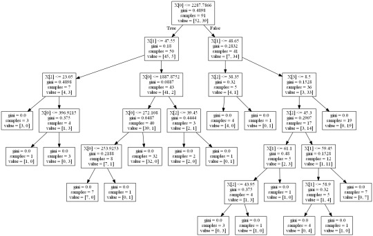
The decision tree analysis was performed to test non-linear relationships among the explanatory variables and a single binary, categorical response variable. The training sample has 91 rows of data and 4 explanatory variables; the testing sample has 61 rows of data, and the same 4 explanatory variables. The decision tree results in 27 true negatives and 16 true positives; and 11 false negatives and 7 false positives. The accuracy score is 70.5%, meaning that the model accurately predicted 70.5% of the internet use rates per country.
1 note
·
View note
Text
Coursera- Machine Learning - Week 1 Assignment
My code:
import pandas as pd import sklearn.metrics from sklearn.model_selection import train_test_split from sklearn.tree import DecisionTreeClassifier
data = pd.read_csv(r'C:\Users\AL58114\Downloads\gapminder.csv', low_memory=False)
data['internetuserate'] = pd.to_numeric(data['internetuserate'], errors='coerce') data['incomeperperson'] = pd.to_numeric(data['incomeperperson'], errors='coerce') data['employrate'] = pd.to_numeric(data['employrate'], errors='coerce') data['femaleemployrate'] = pd.to_numeric(data['femaleemployrate'], errors='coerce') data['polityscore'] = pd.to_numeric(data['polityscore'], errors='coerce')
binarydata = data.copy()
def internetgrp (row): if row['internetuserate'] < data['internetuserate'].median(): return 0 else: return 1
binarydata['internetuserate'] = binarydata.apply (lambda row: internetgrp (row),axis=1)
binarydata_clean = binarydata.dropna()
binarydata_clean.dtypes binarydata_clean.describe()
predictors = binarydata_clean[['incomeperperson','employrate','femaleemployrate','polityscore']]
targets = binarydata_clean.internetuserate
pred_train, pred_test, tar_train, tar_test = train_test_split(predictors, targets, test_size=.4)
print ('Training sample') print (pred_train.shape) print ('') print ('Testing sample') print (pred_test.shape) print ('') print ('Training sample') print (tar_train.shape) print ('') print ('Testing sample') print (tar_test.shape)
classifier=DecisionTreeClassifier() classifier=classifier.fit(pred_train,tar_train)
predictions=classifier.predict(pred_test)
sklearn.metrics.confusion_matrix(tar_test,predictions)
sklearn.metrics.accuracy_score(tar_test, predictions)
from sklearn import tree from io import StringIO from IPython.display import Image out = StringIO() tree.export_graphviz(classifier, out_file=out) import pydotplus graph=pydotplus.graph_from_dot_data(out.getvalue()) Image(graph.create_png())
Results:
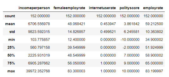
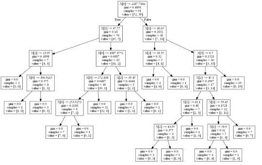
Interpretation:
Decision tree analysis was performed to test non-linear relationships among the explanatory variables and a single binary, categorical response variable. The training sample has 91 rows of data and 4 explanatory variables; the testing sample has 61 rows of data, and the same 4 explanatory variables. The decision tree results in 27 true negatives and 16 true positives; and 11 false negatives and 7 false positives. The accuracy score is 70.5%, meaning that the model accurately predicted 70.5% of the internet use rates per country.
0 notes
Text
Machine Learning for Data Analysis - Week 1
#Load the data and convert the variables to numeric
import pandas as pd from sklearn.model_selection import train_test_split from sklearn.tree import DecisionTreeClassifier import sklearn.metrics
data = pd.read_csv('gapminder.csv', low_memory=False)
data['urbanrate'] = pd.to_numeric(data['urbanrate'], errors='coerce') data['incomeperperson'] = pd.to_numeric(data['incomeperperson'], errors='coerce') data['femaleemployrate'] = pd.to_numeric(data['femaleemployrate'], errors='coerce') data['breastcancerper100th'] = pd.to_numeric(data['breastcancerper100th'], errors='coerce')
#Convert the response variable to binary
binarydata = data.copy()
def urbanGroup (row): if row['urbanrate'] < data['urbanrate'].median(): return 0 else: return 1
binarydata['urbanrate'] = binarydata.apply (lambda row: urbanGroup (row),axis=1)
#Clean the data by discarding NA values
binarydata_clean = binarydata.dropna()
binarydata_clean.dtypes binarydata_clean.describe()
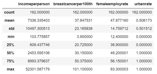
#Split into training and testing sets
predictors = binarydata_clean[['incomeperperson','femaleemployrate','breastcancerper100th']]
targets = binarydata_clean.urbanrate
pred_train, pred_test, tar_train, tar_test = train_test_split(predictors, targets, test_size=.4)
print ('Training sample') print (pred_train.shape) print ('') print ('Testing sample') print (pred_test.shape) print ('') print ('Training sample') print (tar_train.shape) print ('') print ('Testing sample') print (tar_test.shape)
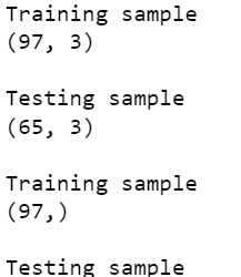
#Build model on the training data
classifier=DecisionTreeClassifier() classifier=classifier.fit(pred_train,tar_train)
predictions=classifier.predict(pred_test)
#Display the confusion matrix
sklearn.metrics.confusion_matrix(tar_test,predictions)

Display the accuracy score
sklearn.metrics.accuracy_score(tar_test, predictions)

#Display the decision tree
from sklearn import tree from io import StringIO from IPython.display import Image from graphviz import Digraph import pydotplus
out = StringIO() tree.export_graphviz(classifier, out_file=out) graph=pydotplus.graph_from_dot_data(out.getvalue()) Image(graph.create_png())
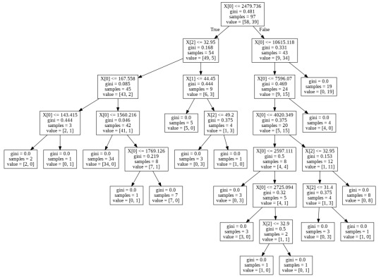
1 note
·
View note
Link
Binary data best website development company in Mohali, India. we provide web development, web design, app development, UI/UX design, digital marketing, ios development, etc. We are focused to create long-lasting relationships with our customers.
contact us:-+91-8699776836 website: https://www.binarydata.in
#best website development company in Mohali#Best Website Development services mohali india#Web design and development in Chandigarh#Web design and development company in india#web design and development services#professional web design and development services
2 notes
·
View notes
Text
RUNNING A RANDOM FOREST:
Machine Learning for Data Analysis
Running a Random Forest
The main drawback to a decision tree is that the tree is highly specific to the dataset it was built on; if you bring in new data to try and predict outcomes, you may not find the same high correlations that your decision tree featured. One method to overcome this is with a random forest. Instead of building one tree from your whole dataset, you subset the data randomly and build a number of trees. Each tree will be different, but the relationships between your variables will tend to appear consistently. In general though, because decision trees are intrinsically connected to the specific data they were built with, decision trees are better as a tool to analyze trends within a known dataset than to create a model for predicting the outcomes of future data.
With those caveats, I decided to build a random forest using the same data as from my previous post, that is, a response variable of internet use rate and explanatory variables of income per person, employment rate, female employment rate, and polity score, from the GapMinder dataset.
Load the data, convert the variables to numeric, convert the response variable to binary, and remove NA values.
In [3]:''' Code for Peer-graded Assignments: Running a Random Forest Course: Data Management and Visualization Specialization: Data Analysis and Interpretation ''' import pandas as pd import numpy as np import matplotlib.pyplot as plt from sklearn.cross_validation import train_test_split import sklearn.metrics from sklearn.ensemble import ExtraTreesClassifier data = pd.read_csv('c:/users/greg/desktop/gapminder.csv', low_memory=False) data['internetuserate'] = pd.to_numeric(data['internetuserate'], errors='coerce') data['incomeperperson'] = pd.to_numeric(data['incomeperperson'], errors='coerce') data['employrate'] = pd.to_numeric(data['employrate'], errors='coerce') data['femaleemployrate'] = pd.to_numeric(data['femaleemployrate'], errors='coerce') data['polityscore'] = pd.to_numeric(data['polityscore'], errors='coerce') binarydata = data.copy() # convert response variable to binarydef internetgrp (row): if row['internetuserate'] < data['internetuserate'].median(): return 0 else: return 1 binarydata['internetuserate'] = binarydata.apply (lambda row: internetgrp (row),axis=1) # Clean the dataset binarydata_clean = binarydata.dropna()
Build the model from the training set
In [10]:predictors = binarydata_clean[['incomeperperson','employrate','femaleemployrate','polityscore']] targets = binarydata_clean.internetuserate pred_train, pred_test, tar_train, tar_test = train_test_split(predictors, targets, test_size=.4) from sklearn.ensemble import RandomForestClassifier classifier_r=RandomForestClassifier(n_estimators=25) classifier_r=classifier_r.fit(pred_train,tar_train) predictions_r=classifier_r.predict(pred_test)
Print the confusion matrix
In [11]:sklearn.metrics.confusion_matrix(tar_test,predictions_r)
Out[11]:array([[22, 5], [10, 24]])
Print the accuracy score
In [12]:sklearn.metrics.accuracy_score(tar_test, predictions_r)
Out[12]:0.75409836065573765
Fit an Extra Trees model to the data
In [13]:model_r = ExtraTreesClassifier() model_r.fit(pred_train,tar_train)
Out[13]:ExtraTreesClassifier(bootstrap=False, class_weight=None, criterion='gini', max_depth=None, max_features='auto', max_leaf_nodes=None, min_samples_leaf=1, min_samples_split=2, min_weight_fraction_leaf=0.0, n_estimators=10, n_jobs=1, oob_score=False, random_state=None, verbose=0, warm_start=False)
Display the Relative Importances of Each Attribute
In [15]:model_r.feature_importances_
Out[15]:array([ 0.44072852, 0.12553198, 0.1665162 , 0.2672233 ])
Run a different number of trees and see the effect of that on the accuracy of the prediction
In [16]:trees=range(50) accuracy=np.zeros(50) for idx in range(len(trees)): classifier_r=RandomForestClassifier(n_estimators=idx + 1) classifier_r=classifier_r.fit(pred_train,tar_train) predictions_r=classifier_r.predict(pred_test) accuracy[idx]=sklearn.metrics.accuracy_score(tar_test, predictions_r) plt.cla() plt.plot(trees, accuracy) plt.ylabel('Accuracy Score') plt.xlabel('Number of Trees') plt.show()
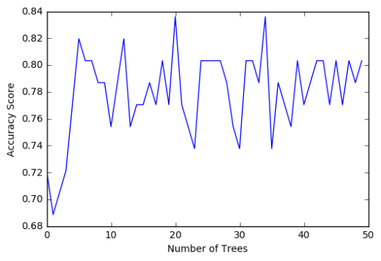
The confusion matrix and accuracy score are similar to that of my previous post (remember, a decision tree is pseudo-randomly created, so results will be similar, but not identical, when run with the same dataset). Examining the relative importance of each attribute is interesting here. As expected, income per person is the most highly correlated with internet use rate, at 54% of the model’s predictive capability. Employment rate (15%) and female employment rate (11%) are less correlated, again, as expected. But polity score, at 20% of the model’s predictive capability, stood out to me because none of the previous models I’ve examined with this dataset have had polity score even near the same level of importance as employment rates. Interesting. Finally, the graph shows that as the number of trees in the forest grows, the accuracy of the model does as well, but only up to about 20 trees. After that, the accuracy stops increasing and instead fluctuates with the random permutations of the subsets of data that were used to create the trees.
0 notes