#chromatic polynomials
Explore tagged Tumblr posts
Visit Tumblr Blog
Explore Tumblr blogs with no restrictions, modern design and the best experience.
Last Seen Tumblr Blogs


Fun Fact
When “GIF” was named word of the year in 2012, Oxford Dictionaries U.S.A. credited Tumblr for pushing the word.
Text
pðltirzzoθzəfməɛŋənb
Pronounced: pthltirzzothzuhfmuhaynguhnb.
Pantheon of: unwholesomeness, insolubility, time, texture, appearance.
Entities
Inrvɪəəoərkrɛaʊəəʌeəb
Pronounced: inrviuhuhouhrkrayowuhuhueuhb Unwholesomeness: perniciousness. Time: geological time. Appearance: hairiness. Legends: group practice, careerism, stem-cell research, brawl. Prophecies: number crunching, jerk, placement, enucleation, talk. Relations: ɪitəvzðftæɛlikisʃəæt (sulfanilic acid), zniɪrɛdkgtðrknɛɪɑrdaɪ (alizarin yellow), oʃinəɪdðɒɑɪstrəfmiŋl (pittance).
Lrtədmertʃnnəinmʊaɪdɪg
Pronounced: lrtuhdmertshnnuhinmooaidig Unwholesomeness: deadliness. Time: musical time. Appearance: disfigurement. Legends: banking game, fraud in law, search, abdominocentesis. Prophecies: human reproductive cloning, ecoterrorism. Relations: ɪitəvzðftæɛlikisʃəæt (cannon cracker).
Mɛðɑiθtwrðɪmtdlɛzbwð
Pronounced: maythahithtwrthimtdlayzbwth Unwholesomeness: jejunity. Time: eternity. Appearance: persona. Legends: acquiring, professional tennis, personification, congregation. Prophecies: wages, hijab, pap test, beating, television program. Relations: ɛŋtiɪnŋtæoəɪæsonnknɪ (ammonia), inrvɪəəoərkrɛaʊəəʌeəb (aldol), ɪitəvzðftæɛlikisʃəæt (turpentine), lrtədmertʃnnəinmʊaɪdɪg (elm).
Oʃinəɪdðɒɑɪstrəfmiŋl
Pronounced: oshinuhidthouahistruhfmingl Unwholesomeness: deadliness. Time: future. Appearance: view. Legends: time, overexposure, conversion. Relations: ənhɪdðswəðnlðgəortɪz (reward).
Vðtʃɪɪɪdʊtismuərutɪɪt
Pronounced: vthtshiiidootismuuhrutiit Unwholesomeness: perniciousness. Time: geological time. Appearance: countenance. Legends: demolition. Prophecies: piracy, course of lectures. Relations: ɪitəvzðftæɛlikisʃəæt (southeast by south), oʃinəɪdðɒɑɪstrəfmiŋl (sorbate), ɛŋtiɪnŋtæoəɪæsonnknɪ (internal revenue), inrvɪəəoərkrɛaʊəəʌeəb (reciprocality).
Zniɪrɛdkgtðrknɛɪɑrdaɪ
Pronounced: zniiraydkgtthrknayiahrdai Unwholesomeness: unhealthfulness. Time: continuum. Appearance: superficies. Legends: exchange, carving, vigilantism. Prophecies: allocution, purge, coup d'etat, strip mining, lockstep.
Ənhɪdðswəðnlðgəortɪz
Pronounced: uhnhidthswuhthnlthguhortiz Unwholesomeness: deadliness. Time: duration. Appearance: view. Legends: shoot, pigsticking, disownment, affairs, self-assertion. Prophecies: swimming meet, withdrawal, deviationism, inscription, electric shock. Relations: ɛŋtiɪnŋtæoəɪæsonnknɪ (shoe leather), lrtədmertʃnnəinmʊaɪdɪg (abruptness), zniɪrɛdkgtðrknɛɪɑrdaɪ (petrochemical), oʃinəɪdðɒɑɪstrəfmiŋl (pinot blanc).
Əɪtmtəsgtzɪŋðmɪlraʊən
Pronounced: uhitmtuhsgtzingthmilrowuhn Unwholesomeness: harmfulness. Time: geological time. Appearance: hairiness. Legends: proclamation, budget cut, contortion, air reconnaissance. Prophecies: obviation, repositing, drip. Relations: ɛŋtiɪnŋtæoəɪæsonnknɪ (homogeneous polynomial), inrvɪəəoərkrɛaʊəəʌeəb (baronetcy).
Ɛŋtiɪnŋtæoəɪæsonnknɪ
Pronounced: ayngtiinngtaouhiasonnkni Unwholesomeness: deadliness. Time: future. Appearance: color. Legends: base on balls, stridulation, stimulation, monte. Relations: inrvɪəəoərkrɛaʊəəʌeəb (chromate), lrtədmertʃnnəinmʊaɪdɪg (omega-6 fatty acid), mɛðɑiθtwrðɪmtdlɛzbwð (reciprocal), zniɪrɛdkgtðrknɛɪɑrdaɪ (linear operator).
Ɪitəvzðftæɛlikisʃəæt
Pronounced: iituhvzthftaaylikisshuhat Unwholesomeness: putrescence. Time: civil time. Appearance: homeliness. Legends: by-election, communications technology, whitewash, random sampling, keynote speech. Prophecies: naturalization, derivation, harakiri, sonic boom, abbreviation. Relations: zniɪrɛdkgtðrknɛɪɑrdaɪ (vinegar).
0 notes
Text
Complexity of calculating, complexity of things
To follow up on this post: we had a complexity axiom that told us something about topology, apparently. I would like to elaborate on this and explain what it's "really" (in my opinion) doing. The topological statement is also, inherently, a complexity question. It's just that, instead of being couched in the usual langauge of minimum complexity of a Turing machine calculating something, it's a statement about the minimum complexity writing down a description of some knot. This is more natural than you might think!
Morally, it's very analogous to the "theorem" that the Hajos number of a graph can be exponentially big (under the complexity "axiom" that coNP != NP). The Hajos number is one way of measuring how hard to build a graph from simpler graphs. You start with complete graphs K_n. Of the steps you're allowed to use, none of them can ever decrease the chromatic number of the graph. It's also been shown you can always build a graph in this way where the chromatic number never changes. That is, the Hajos number sort of asks: how many steps do you need to build this graph, in a way where each step leaves the chromatic number unchanged?
So, if you have a graph that is "simple" by measure of the Hajos number (at most polynomially long), then it means that there's a short proof (a polynomial length sequence of steps to construct it) that it has a certain chromatic number k. This means there is no coloring of k, which is coNP-hard. So you would have a NP way to check coNP questions.
Generally you could imagine other versions of this... like, #3COL is the counting problem that asks how many 3-colorings there are of a graph. This is #P-hard, so if P^{#P} != NP, then this shouldn't be in NP. If I gave you a set of allowed "moves" to do on a graph that always change #3COL in simple ways (e.g. "I'm going to add a degree-one edge, which doubles the number" or "This graph has two distinct components, so I can reduce to counting on each component separately and then multiply"). Then I define the complexity of a graph com(G) as the number of steps it takes to reduce it to the empty graph. P^{#P} != NP would imply that com(G) must grow superpolynomially in the size of G.
I could generalize that somewhat. Instead of reducing to just trivial graphs, I could say, I want to reduce to graphs of small treewidth. This is 'enough' because on graphs of small treewidth, #3COL is easy to compute. Maybe the steps I'm allowed to use won't reduce treewidth, but I'm just sort of asking: can I take a graph and somehow canonicalize it to a graph of small twin-width that has the same number of colorings?
So if I start a graph G and can reach a graph H by applying these moves, then I say that G and H are "equivalent" within this space of moves. The distance(G,H) is how many moves you need to do this. I would be able to solve #3COL quickly on G if I can reduce it to H with only polynomially many moves, and then H has small treewidth. So then the theorem would be,
if there is a constant k such that (for all G, there is an equivalent H, with polynomial distance(G,H), and treewidth(H) <= k), then P^{#P} = NP.
so by flipping that around,
P^{#P} != NP --> for any k, there is some G, for which all equivalent H, either have treewidth(H) > k, or a superpolynomial distance(G,H).
This paper from Freedman is looking at a particularly nice, maybe natural example of this. Here instead of #3COL of a graph, the hard thing to calculate is the Jones polynomial of a knot. The allowed "steps" to change the knot are the standard Reidemeister moves together with Dehn surgery. Instead of talking about graphs of small treewidth, the measure of "complicated" knots is the girth of their plane diagram. The theorem there is
P^{#P} != NP --> for any b and b', there is some D, for which all equivalent D', either have girth(D') > b*log(size(D)) + b', or a superpolynomial distance(G,H).
#math#complexity-theory#coloring#it's funny because it's a tumblr tag so it's “hashtag-coloring” but also we're talking about the counting version of the 3-coloring problem
1 note
·
View note
Text
Chromatic Polynomials & Why They’re Cool
Super Quick Note: This post features LaTeX code, and will be better read directly on my blog, although it should be relatively readable on your dash!
Okay, so what are chromatic polynomials?
Given a graph $G$, a chromatic polynomial of $G$, denoted $\chi_G(k)$ is a polynomial that outputs the number of proper $k$-colorings of $G$, when $k$ is the number of colors we are given.
Okay, so really, what are chromatic polynomials?
Let’s break down the definition. First, let’s talk in general about graphs. What is a graph? A graph is a collection of points called vertices connected by edges. An example of a graph (this graph has a special name: the Petersen graph) is below:
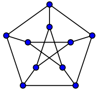
Now, let’s say we want to color the vertices of this graph such that no two adjacent vertices (meaning vertices that are connected by an edge) share the same color. This is called a proper coloring of the graph. Additionally, let’s say that we’re only allowed to use $k$ colors. If we have a proper coloring using $k$ colors, we call it a proper $k$-coloring.
Let’s revisit the definition of our chromatic polynomial. Given our input $k$ is the number of colors, the chromatic polynomial outputs the number of different proper $k$-colorings.
How do we find the chromatic polynomial?
Well, there’s a couple different ways to find them. Let’s look at finding the chromatic polynomial for different complete graphs. (A complete graph $K_n$ is a graph of $n$ vertices where every vertex is adjacent to every other vertex.)
Let’s take a look at the picture below, which shows $K_1$, $K_2$, and $K_3$.
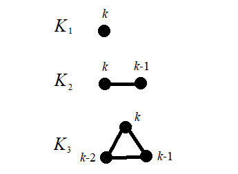
What do all these $k$’s by the vertices mean? Let’s suppose we’re given $k$ colors to color each vertex. Pick a vertex of the complete graph to start at. That vertex has a possible $k$ colors it can be. We’re off to a great start! Now pick a vertex adjacent to the first vertex. Since we already took one color for that vertex, we have $k$-1 remaining colors for the current vertex. We continue this pattern until we’re out of vertices. Then what we’ll do is multiply all the values of the vertices together -- and voila, we have our chromatic polynomial.
For example, consider the $K_3$ above. It’s chromatic polynomial, $\chi_{K_3}(k)$, is equal to $k(k-1)(k-2)$. And in fact, for a general $K_n$, the chromatic polynomial, $\chi_{K_n}(k) = k(k-1)(k-2)\cdots(k-n+1)$. This function will tell us how many proper colorings we can get for $K_n$ given $n$ vertices and $k$ colors! How cool!
The process for finding the chromatic polynomial for other (non-complete) graphs is a bit trickier and hinges on something called the Deletion-Contraction Algorithm, also known as the Fundamental Reduction Theorem. While I won’t get into that in this post, if you’re interested in chromatic polynomials, it’s definitely something to check out.
Okay, but really, why is this cool?
The real “cool factor” of chromatic polynomials comes into play when we talk about why they were even created. Chromatic polynomials were originally created by George David Birkhoff in 1912 in an attempt to prove the Four Color Theorem. If he could show that $\chi_G(4)>0$, where $G$ is planar (that is, it can be drawn with no edge crossings), then the Four Color Theorem would be proven. And while the Four Color Theorem ended up being proven in another way, chromatic polynomials still remain Pretty Damn Cool and are an important aspect of algebraic graph theory.
(I’m also pretty biased, since my current thesis research is regarding graphs whose chromatic polynomials have integer roots.)
Thanks for reading!
I hope all is well with you! As always, feel free to send me a message/ask/reply/whatever with any questions, comments, or concerns! Stay positive! <3
References:
Chromatic Polynomial History
49 notes
·
View notes
Text


Ruth Aaronson Bari, regular major maps of at most 19 regions and their Q-chromials
#4-color theorem#graph theory#George David Birkhoff#Bill Tutte#W. H. Tutte#Tutte polynomial#chromatic polynomial#polynomials#algebra#graph colourability#4-colour theorem#sphere#S2#genus zero#surfaces#manifolds#topology#mathematics#maths#math#Birkhoff#G. D. Birkhoff#Ruth Aaronson Bari#Potts model#spinors#spin networks#networks#network theory#connectivity#connectedness
48 notes
·
View notes
Text
Acton blink lite synching

#Acton blink lite synching free
The application of WFC technology in an off-axis three mirror anastigmatic (TMA) system has been proposed, and the design and optimization of optics, the restoration of degraded images, and the manufacturing of wavefront coded elements have been researched in our previous work. This technology has been applied in many imaging systems to improve performance and/or reduce cost. Wavefront coding ( WFC) is a kind of computational imaging technique that controls defocus and defocus related aberrations of optical systems by introducing a specially designed phase distribution to the pupil function. Moreover, we fabricated a demonstration set assuming the use of a night vision camera in an automobile and showed the effect of the WFC system.Įxperimental study of an off-axis three mirror anastigmatic system with wavefront coding technology. As a result, the effect of the removal of the chromatic aberration of the WFC system was successfully determined. We acquired images of objects using a WFC camera with this lens under the conditions of visible and infrared light. Our original annular phase mask for WFC was inserted to the lens, for which the difference between the focal positions at 400 nm and at 950 nm is 0.10 mm. We perform an experiment of achromatic imaging with wavefront coding ( WFC) using a wide-angle automobile lens. Ohta, Mitsuhiko Sakita, Koichi Shimano, Takeshi Sugiyama, Takashi Shibasaki, Susumu Visible-infrared achromatic imaging by wavefront coding with wide-angle automobile camera
#Acton blink lite synching free
Nevertheless, the best results are obtained by using the trefoil phase-mask, because the decoded image is almost free of artifacts. Numerical results show defocus invariance aberration in all cases. WFC systems were simulated using the cubic, trefoil, and 4 Zernike polynomials phase-masks. In this, the merit function minimizes the mean square error (MSE) between the diffraction limited Modulated Transfer Function (MTF) and the MTF of the system that is wavefront coded with different misfocus. In this paper, the optimization of the phase deviation parameter is done by means of genetic algorithms (GAs). For years, several kinds of PM have been designed to produce a point spread function (PSF) near defocus-invariant. Wavefront Coding ( WFC) systems make use of an aspheric Phase-Mask (PM) and digital image processing to extend the Depth of Field (EDoF) of computational imaging systems. So, you can easily avail their service options free of charge within the warranty period.Optimization of wavefront coding imaging system using heuristic algorithms Acton provides a 6-month warranty period for the skateboard and other in-box accessories.It also prevents toppling over when the skateboard comes to a sudden stop. This ensures that your brakes are functional in regenerating electric power for the wheels. Due to its single hub motor system, Acton includes regenerative braking in this model.In addition to that, 2 side lights are also incorporated for better visibility while commuting. Acton also provides integrated LED lights on its front and back.The construction of this skateboard is pretty sturdy and its 83 mm wheels improve the overall stability and maneuverability of this long board.Some of its other safety considerations are as follows: In addition to that, the Blink S has been certified safe for air travel, so you can easily carry this board with you in cross-country trips. If you are wondering how safe this Acton Blink S is, then you would be glad to know that this model has one of the highest safety ratings from critical reviews in the market.
0 notes
Text
Graphs are actually just one type of object that can define more general structures called matroids. Consider, for example, points on a two-dimensional plane. If more than two points lie on a line in this plane, you can say that those points are “dependent.” Matroids are abstract objects that capture notions like dependence and independence in all sorts of different contexts — from graphs to vector spaces to algebraic fields.
Just as graphs have chromatic polynomials associated with them, there are equations called characteristic polynomials attached to matroids. It was conjectured that the polynomials for these more general objects should also have coefficients that are log concave. But the techniques Huh used to prove Read’s conjecture only worked for showing log concavity for a very narrow class of matroids, such as the matroids that arise from graphs.
With the mathematician Eric Katz, Huh broadened the class of matroids such a proof could apply to. They followed a recipe of sorts. As before, the strategy was to start with the object of interest — here, a matroid — and use it to construct an algebraic variety. From there, they could extract an object called a cohomology ring and use some of its properties to prove log concavity.
There was just one problem. Most matroids don’t have any sort of geometric foundation, which means there’s not actually an algebraic variety to associate to them. Instead, Huh, Katz and the mathematician Karim Adiprasito figured out a way to write down the right cohomology ring straight from the matroid, essentially from scratch. They then showed, using a new set of techniques, that it behaved as if it had come from an actual algebraic variety, even though it hadn’t. In doing so, they proved log concavity for all matroids, resolving the problem known as Rota’s conjecture once and for all. “It’s pretty remarkable that it works,” Baker said.
The work showed that “you don’t need space to do geometry,” Huh said. “That made me really fundamentally rethink what geometry is.” It would also guide him toward a host of other problems, where he continued to push that idea further, allowing him to develop an even broader range of methods.
But for all the specificity the work requires, building the right cohomology ring requires massive amounts of guesswork and groping around in the dark. It was an aspect of the work that Huh particularly enjoyed. “There is no guiding principle … no clearly defined goal,” he said. “You just have to make a guess.”
That lack of intention precisely mirrors how he functions best in his day-to-day life, too. It was as if he’d uncovered a mathematical program that perfectly fit his personality. Once again, he found that “things just happen by themselves,” Huh said.
He dropped out to become a poet – now he’s won a Fields Medal
https://www.quantamagazine.org/june-huh-high-school-dropout-wins-the-fields-medal-20220705/
Comments
1 note
·
View note
Text
(Long) Detailed Proof of Kőnig's Lemma (Explicit, Down to Axiom of Choice)
Kőnig's Lemma states that in an infinite, locally finite, connected graph $G$, there exists an infinite one-way path (a ray). The proof of it in my graph theory book (Introduction to Graph Theory, 4th ed., Wilson) had a sour taste to it, like it was covering something up. So I checked out proofs from other sources, which also seemed to cover up something which felt very close to the foundation (i.e. using the axioms). After looking it up I found out that this is indeed the case, as it results directly from the axiom of dependent choice (DC).
This wasn't a question on an assignment for me or anything, but I wanted to try to give a more detailed, albeit lengthy proof of the lemma with more explicit constructions and play-by-play, highlighting some of the key points and bare bones math going on here (including the general statement of the lemma and the use of DC), to the best of my understanding. I was hoping that anyone with time to spare hands could review or give comment, make sure everything I'm stating things correctly! And of course, I would be happy if this helps anyone in a similar predicament that comes to read this in the future, or helps anyone to appreciate the deeper levels of a simple theorem.
I've enabled the "answer your own question" box so I can post my proof separately, but I encourage/challenge others to do the same and make a detailed construction as an exercise, especially during these times of isolation!
Below I'll prove a similar theorem which uses Kőnig's Lemma in a more general form (but sweeps DC under the rug). It's a good reference because it's easier to understand without a super explicit construction:
Let $G$ be a countable graph such that every finite subgraph of $G$ is $k$-colourable. Then $G$ is $k$-colourable.
Proof
Since $G$ is countable, its vertices are enumerable as $v_1$, $v_2$, $v_3$, etc. Let $G_n$ be the (finite) subgraph induced by vertices $v_0$ through $v_n$. Since each vertex $v_n$ corresponds to a finite induced subgraph $G_n$, there are countably many $G_n$. Since $G_n \subset G_{n+1}$ for all $n$ by construction, the union over all $G_n$ yields $G$. Since each $G_n$ is finite, there are countably many corresponding sets $C_n$ of valid $k$-colourings of $G_n$, each non-empty with a finite number of elements given by the chromatic polynomial of $G_n$, $P_{G_n}(k)$. If we consider a colouring of $G_{n+1}$ and remove vertex $v_{n+1}$, we are left with a valid colouring of $G_n$: removing vertices does not invalidate a colouring. And so this valid colouring of $G_n$ must be an element of $C_n$. In general, for every colouring $c_{n+1} \in C_{n+1}$ of $G_{n+1}$ there is some colouring $c_{ind} \in C_{n}$ such that $c_{ind} \prec c_{n+1}$ (i.e. $c_{ind}$ is induced on $G_n$ by $c_{n+1}$). Kőnig's Lemma states that since there are countably many non-empty $C_n$ that follow these conditions, we must have a countable set of $c_n \in C_n$ such that $c_n \prec c_{n+1}$ for all $n$. If there were not, then all inductive sequences of colourings would terminate at some finite point $t$. If we take $\tau$ to be the maximum such $t$ over all sequences, then $C_{\tau + 1}$ must be empty, contradictory to our assumption that all $G_n$ are $k$-colourable (and in turn that all $C_n$ are non-empty). Therefore there is a countable set of inductive valid $k$-colourings $c_n$, and their union gives us a valid $k$-colouring of $G$.
Thus, $G$ is $k$-colourable. $\blacksquare$
The general form of Kőnig's Lemma can be stated as follows (paraphrasing Infinite Graphs - A Survey, by Nash-Williams, 1967):
Given a countable sequence of finite, non-empty, disjoint sets $S_n$ and a relation $\prec$ on $\bigcup S_n$, if for each element $s_{n+1} \in S_{n+1}$ there exists an $s_n \in S_n$ such that $s_n \prec s_{n+1}$, then there exists a countable sequence of elements $(s_n)$ such that $s_n \prec s_{n+1}$ for all $n$.
The end of the $k$-colouring proof I gave is basically the proof of this theorem. In this general form, the $S_n$ can be thought of as "configuration spaces" (finite sets of valid configurations), and the relation $\prec$ can be thought of as an inductive consistency relation. In the $k$-colouring proof, our configuration spaces are the $C_n$ and they are finite due to the chromatic polynomial of $G_n$, though I didn't explicitly construct them so we can't show that they are disjoint. But as I mentioned, this is still easier to understand without explicit construction. This is because we iterate out $G$ vertex by vertex, and as a result, we get a natural correspondence between the iterated subgraphs and their colourings. In proving the graph theoretic result about the existence of an infinite one-way path, the iteration scheme is not vertex by vertex, and so more explicit construction is needed to make the simple argument as above. That will be in my proof below, and similar methods can be used to construct a more explicit proof of this $k$-colourability result, and one for planarity as well!
from Hot Weekly Questions - Mathematics Stack Exchange
from Blogger https://ift.tt/34nujYj
0 notes
Text
Anritsu MW9076D SM Fiber Optic OTDR
Welcome to a Biomedical Battery specialist of the Anritsu Battery
The Anritsu MW9076 series is a small and lightweight optical time domain reflectometer (mini-OTDR) for measuring loss and locating faults in optical fiber cables at fiber installation and maintenance. It has excellent basic performance specifications including a dynamic range of 45 dB and a world-beating backscatter dead zone of just 8 m. For the best price performance, the series includes four types of main frame, two types of optical channel selector unit and two types of display unit.
Features
•8 m short dead zone
•Simple measurement of chromatic dispersion from one end of optical fiber
•Measurement in 10 s (Full-Auto mode), 0.15 s real-time sweep
•5 cm high resolution, 50,000 sampling points
•8.4 inch TFT-LCD color display with battery such as Anritsu MS2721A Battery, Anritsu MS2724B Battery, Anritsu MS2722C Battery, Anritsu MS2726C Battery, Anritsu MS2711E Battery, Anritsu MS2712EC Battery, Anritsu MT8212E Battery, Anritsu MS2024A Battery, Anritsu MS2026A Battery, Anritsu MS2036A Battery, Anritsu MS2025B Battery, Anritsu MS2026B Battery
Performance and Functions
•High dynamic range
When using a wavelength of 1.55 µm, a point about 190 km distant can be measured.
•Short dead zone
Clearly measure up to near end by 8 m dead zone (back-scatter, SM unit)
•Chromatic dispersion measurement
The MW9076D has a built-in function for measuring chromatic dispersion even outdoors. The chromatic dispersion can be measured automatically over a wide range from 1300 to 1660 nm from one end of the fiber. The dispersion reproducibility is ±0.05 ps/(nm · km)* and the dynamic range is 30 dB. The MW9076D can be operated from an external PC using remote commands to measure the chromatic dispersion. For detail of the chromatic dispersion measurement, refer to the document of “product introduction MW9076 series Optical Time Domain Reflectometer”.
*: Measured with 25 km of 1.3 µm zero-dispersion fiber (ITU-T G.652) at 1550 nm.
•Fresnel reflection
The far-end Fresnel reflection can be measured for four wavelengths (1310/1450/1550/1625 nm).
•Group delay characteristics
The fitting formula supports cubic or quintic Sellmeier, and polynomials can be applied to various types of fibers.
•Chromatic dispersion characteristics
The zero and total dispersion can be displayed along with the delay, dispersion and dispersion slope at 0.1 nm steps.
•High-speed measurement
It takes only 10 seconds to measure and display the waveform and connection loss on one screen. Just one press of the Start key is all that is needed to make measurement.
•Full automatic mode
Measurement results are displayed by simply pressing the Start key. All complicated settings of distance range, pulse width, attenuator, and maker can be automatically executed. Measurement speed in this mode was significantly increased. When the wavelengths are set to ALL, wavelengths are automatically changed.
0 notes
Text
my abstract was accepted!
If anyone’s going to the Trisection Meeting in Indiana at the end of this month-- come see my talk! :) (schedule pending)
Chromatic Polynomials, Counterexamples, and Conjectures
The chromatic polynomial of a graph $G$, denoted $\chi_G(k)$, is the function which to each natural number $k$, returns the number of proper $k$-colorings of $G$. A large family of graphs can have their chromatic polynomials determined by the multiplication principle -- for example, the chromatic polynomial of the complete graph on 4 vertices is $k(k-1)(k-2)(k-3)$, since we can choose any one of the $k$ colors for the first vertex, leaving $k-1$ allowable colors for the second vertex, and so on. The graphs for which this technique works are called chordal graphs, and it is easy to see that the roots of all of their chromatic polynomials are integers. A natural conjecture is the converse, i.e., that having $\chi_G(k)$ with all integer roots implies that $G$ is chordal. This question was open until 1975, when Read found an explicit counterexample. We'll address some refinements of the conjecture, focusing on a specific conjecture by Dong and Koh conditioning the result on the graph's chromatic number.
11 notes
·
View notes
Text
(Chromatic Quasisymmetric Functions and Regular Semisimple) Hessenberg Varieties II
This conference-winning talk was given by John Shareshian at the 2017 Midwest Combinatorics Conference, and if you’re wondering when you missed Part I, the answer is that you didn’t— I did (that was the talk I slept through). The good news is that whatever the first part of the talk was about, missing it didn’t really interfere with the story he was putting on the board (at least until the end, when I was lost for unrelated reasons and so it didn’t matter :P)
As you can probably tell from the title, this is not the most elementary talk that there ever was. I would refer newer readers to my sequence on Schubert varieties, which more or less forms the background for this talk.
------
The star of this talk is the titular Hessenberg varieties, which are a class of subvarieties of the (complete) flag variety. I am not entirely sure whether every Hessenberg variety is a Schubert variety, although there certainly some Hessenberg varieties which are Schubert varieties. In any case, the definition goes as follows:
Definition. A vector $m\in\Bbb N^n$ is called a Hessenberg function if $i\leq m_i\leq m_{i+1}\leq n$ for all $i$. Then, given a Hessenberg function $m$ and a linear transformation $X$ on $\Bbb C^n$, the Hessenberg variety is a subset of the flag variety containing those flags $0\subset F_1\subset\cdots\subset F_{n-1}\subset\Bbb C^n$ which satisfy the additional inclusions $XF_i\subset F_{m_i}$.
Playing with these conditions a bit can be instructive. In the trivial case where $X$ is the identity, we simply recover the flag variety, because the “additional” inclusions are already encoded in the flag. In the other trivial case where the Hessenberg function is $(n,n,n,\cdots, n)$, we also get the flag variety, because the additional inclusions simply say that $X$ must send the subspace somewhere in $\Bbb C^n$ (i.e., they say nothing).
So already we see that this construction is going to be slightly annoying, since we can obtain the same variety in multiple ways. But, pressing onward to the other extreme Hessenberg function $(1,2,3,\dots, n)$, we already start to see interesting behavior. For instance, if
$$ X = \begin{bmatrix} 1 && \\\ & 2 & \\\ && 3 \end{bmatrix}, $$
then the Hessenberg variety is a $\Bbb P^1$ with three special points at which an additional $\Bbb P^1$ has been attached. This is actually not terrible to calculate by hand:
The data of the flag is specified by the single inclusion $F_1\subset F_2$ for $1$-or-$2$-dimensional subspace $F_1$ or $F_2$.
If $F_1$ is not an eigenspace of $X$, then this means that $F_2$ must contain both $F_1$ and the distinct space $XF_1$. Since $F_2$ is two-dimensional, this completely determines $F_2$.
If $F_1$ is an eigenspace of $X$ (of which there are three), then $XF_1=F_1$ and so we must choose another vector to form the other basis element of $F_2$.
Therefore, there is a $\Bbb P^1$ worth of choices (for $F_1$), except that three of those choices give an additional $\Bbb P^1$ worth of choices.
Historically, these were first studied by DeMari and Shayman, and later Procesi, who were primarily interested in applications. In particular, they determined that these varieties are equipped with a torus action with finitely many fixpoints and one-dimensional orbits, and that it is a finite-dimensional complex projective variety. Therefore, the GKM theory applies, and thus the combinatorics appears: calculating the equivariant cohomology is equivalent to calculating splines over a particular graph (generalized in the sense that the underlying ring is $R=\Bbb C[t_1,\dots, t_n]$).
That graph is actually quite easy to describe. For any Hessenberg function $m$, we say that its Hessenberg graph has vertices $\{1,2,3,\dots n\}$, and there is an edge between $i$ and $j$ whenever $i<j\leq m_i$ (or $j<i\leq m_j$; the graph is not directed).
It turns out that the ring of splines on the Hessenberg graph is actually an $\Bbb CS_n$-module, and we can write down its Frobenius character using the chromatic symmetric polynomial of the Hessenberg graph. Thus... something about Schur positivity— look, I don’t get it either. I’ve just heard the words enough to feel confident nodding my head.
Something that I do understand, and seems to be at least slightly nontrivial, is this: the Hessenberg graph depends only on the Hessenberg function, but its ring of splines in principle depends on the entire Hessenberg variety. We have already seen at least one instance in which the variety can be formed with two distinct functions, and hence is associated to two distinct graphs. But since the ring of splines is a purely graph-theoretic construction, it should a priori depend on the choice of graph. It seems to me, therefore, that Hessenberg varieties might serve as a (ridiculously high-tech) machine for finding pairs of graphs with the same ring of splines? It would be kind of fun to chase that idea down...
#math#maths#mathematics#mathema#combinatorics#geometry#geometric combinatorics#algebraic combinatorics#graph theory#mcc#mcc2017#this is also the last talk of mcc2017#but we already did the miscellany so no fanfare on this one :P
2 notes
·
View notes
Text
Chromatic polynomials are definitely a nice thing to learn about and share! :)
hey all :)
slides for my talk this weekend at the MAA Trisection Meeting are available here if you’re interested!!
have a great day!!!
19 notes
·
View notes
Text
Miscellany from the MCC 2015
So... remember that conference that I went to 18 months ago?
Well, I’m going to wrap those posts up, finally XD
(Actually, I procrastinated this so long because my organizational scheme was bad and I thought I had quite a few more posts left, but it turns out there are only four talks that I didn’t already write up. One of them I slept through; the other three I’ll write about here.)
------
Matthew Dyer, Poincaré Series of Coxeter Groups and Multichains in Eulerian Posets.
At the time I wrote this post, I had no idea what a Coxeter group was, and had never seen any algebraic number theory— not even the Brubaker talks that showed up in this conference. So this talk caught me completely unawares. I wasn’t able to understand much of anything and my notation that I copied down contains obvious errors. However, in retrospect: a Poincaré series is a particular type of modular form, and it seems like he was doing something with parabolic subgroups. The relation to Eulerian posets probably comes from the fact that the Bruhat order is an Eulerian poset, but it’s not clear to me at what generality he was attempting to write his results.
Martha Yip, A Categorification of the Chromatic Symmetric Function. She cited Radmila Sazdanovic as a collaborator.
Although my notes for this talk are also subpar, I was able to understand at least a little bit of what was going on, and write down enough that present-me understands even a little bit more :) The chromatic symmetric function for a given graph $G$ is defined as $$ \sum_{\kappa \text{ coloring of } G} x_{\kappa(v_1)}x_{\kappa(v_2)}\cdots x_{\kappa(v_n)}. $$
The goal of the talk was to recognize this function the graded Frobenius character of some homology theory. A hint in this direction is supposedly given by the Murnaghan–Nakayama rule; she said this suggests a plan for usefully turning edges of the graph into vector spaces.
I mentioned in my notes, and so it’s probably worth saying that the Q&A session for Yip’s talk was very lively. It seemed like they had been able to make things work, but hadn’t “explored the territory” much, because she had to answer many of the questions with “I don’t know”. In any case people seemed to be rather excited about it— at the time I wasn’t, but I think that I appreciate the appeal more now.
Aaron Lauve, Characteristic Polynomial of the Antipode for Combinatorial Hopf Algebras. He cited Marcelo Aguiar as a collaborator.
So I don’t have anything to say about this talk, except two tiny remarks. First, Dennis Stanton (professor at UMN, hypergeometric series specialist, and one of the two instructors for the combinatorics class last year) asked if, by choosing a particular Hopf algebra, we could recover the Rogers-Ramanujan identities. Lauve didn’t know, but “he said some things and Stanton seemed happy”.
Second, I wish had managed to take better notes for this talk because I’ve recently become interested in Aguiar’s line of work :)
#math#maths#mathematics#mathema#number theory#coxeter groups#symmetric functions#combinatorics#algebraic combinatorics#mcc#mcc2015
0 notes
Text
Observations from SEICCGTC 2017 Part 6
There were a lot of talks at this conference; while I understood most of them pretty well, there were also many which were not amenable to my taking notes (see Day 1 for the longer explanation). Hence, my usual “Miscellany” posts have become these “Observations”. To keep things brief, I will refrain from giving many background definitions; providing links instead where appropriate.
(More observations: 1 2 3 4 5 6 7 8)
[ When the presenter’s name does not have an associated link, I could not find an academic website for them. ]
------
Jason Brown, Recent Results on Chromatic Polynomials
Here is a fairly established conjecture in graph theory: If $G$ is an $n$-vertex connected graph with chromatic number $k$, then the chromatic polynomial evaluated at any positive integer $m$ satisfies $$\chi_G(m) \leq m(m-1)(m-2)\cdots(m-k+1)\cdot (m-1)^{n-k}.$$ Brown proved that this conjecture is true if $m$ is sufficiently large. This doesn’t reduce the problem to a large case check, though: the bound on $m$ depends on $k$.
In a rather different direction, there have also been recent advances in analyzing the polynomials’ roots, which are generally not real: in fact, random graphs have non-real roots of their chromatic polynomials with probability $1$. Brown showed that if $G$ has chromatic number at least $n-3$, then the real parts of $\chi_G$ are at most $n-1$, and there are roots whose imaginary parts are grow linearly with $n$. Sokal gives a weak estimate for the constant that governs this linearity: the absolute value of the roots (and hence the imaginary parts) are at most $8n$.
In sketching the proof of his real-part result, he went out of his way to mention the Gauss-Lucas theorem as a generalization Rolle’s theorem to the complex plane, which is often useful but underutilized.
Amin Bahmanian, On the Existence of Generalized Designs
A $(n,a,h,\lambda)$-design is an $n$-vertex hypergraph in which every edge has $a$-elements, and every size-$h$ subset belongs to exactly $\lambda$ edges. This is equivalent to producing a decomposition of $\lambda K_n^h$ into $K_a^h$, where $c K_x^h$ is the hypergraph containing $c$ copies of all size-$h$ subsets of the $x$ vertices.
For general parameters $n,a,h$, and $\lambda$, there may not be any designs: indeed there are certain standard divisibility conditions among these numbers which must hold. The rest of the talk that made any sense to me was a history of existence results.
Supposing that the “standard divisibility conditions” hold, then $(n,a,h,\lambda)$-designs exist... whenever $n$ is sufficiently large and $h=2$ (Wilson 70s); for all $a,h$ and at least one $\lambda$ (Teirlinck 80s); for all sufficiently large $n$, where the bound may depend on $a,h$, and $\lambda$ (Keevash 2014).
Also, in the 80s, Rödl showed that for all $a$ and $h$, there is an $(n,a,h,1)$-“almost design”, in a way that Bahmanian left unspecified. And, most recently Bahmanian himself used Keevash’s theorem (or at least the same ideas) to show a “multipartite version”: for all $m,a,h$, and $\lambda$, and all sufficiently large $n$ (possibly depending on $a,h$, and $\lambda$) there is a decomposition of $\lambda K_{n,n,\dots, n}^h$ into copies of $K_{m,m,\dots, m}^h$, where the numbers of $n$’s and $m$’s are both $a$.
[ Previous ] [ Post 6 ] [ Next ]
#math#maths#mathematics#mathema#graph theory#algebraic graph theory#hypergraph theory#bahmanian's talk almost got its own post#but I think if I were to expand on it#I would need to learn quite a bit about design theory#since what's in this post is darn close to the extent of what I know#seiccgtc#seiccgtc2017
0 notes
Note
ah okay! i am actually familiar with chromatically unique graphs but wasn’t sure if that fit in with what you had asked about :) it’s all cool stuff!
my undergrad thesis was on chromatic polynomials :)
Have you done much work with unique determination of graphs? I've been mostly fixated on that topic since I've started working at graph theory things. If you have, do you have a favorite metric for it?
I haven’t worked with that, unfortunately. I’m actually not very familiar with it. If you have any cool papers or resources though, send em my way! I’d love to learn!
15 notes
·
View notes
Note
hey no worries here! i think it’s great you included the link!
my thesis focused on chromatic polynomials that have only integer roots. particularly those of graphs with chromatic number less than or equal to 4. there’s a conjecture that states if a graph has a chromatic polynomial with only integer roots and its chromatic number is less than or equal to 4, it is a chordal graph (no induced cycle of length four or greater)! my thesis explores this conjecture. chromatically unique graphs come in handy in the case where the chromatic number is 3 :)
Have you done much work with unique determination of graphs? I've been mostly fixated on that topic since I've started working at graph theory things. If you have, do you have a favorite metric for it?
I haven’t worked with that, unfortunately. I’m actually not very familiar with it. If you have any cool papers or resources though, send em my way! I’d love to learn!
15 notes
·
View notes