#difference between zeros and ones arrays in python numpy | Explore Tumblr posts and blogs

marialaura-diazpena · 4 years ago

Text

My Programming Journey: Understanding Music Genres with Machine Learning

Artificial Intelligence is used everyday, by regular people and businesses, creating such a positive impact in all kinds of industries and fields that it makes me think that AI is only here to stay and grow, and help society grow with it. AI has evolved considerably in the last decade, currently being able to do things that seem taken out of a Sci-Fi movie, like driving cars, recognizing faces and words (written and spoken), and music genres.

While Music is definitely not the most profitable application of Machine Learning, it has benefited tremendously from Deep Learning and other ML applications. The potential AI possess in the music industry includes automating services and discovering insights and patterns to classify and/or recommend music.

We can be witnesses to this potential when we go to our preferred music streaming service (such as Spotify or Apple Music) and, based on the songs we listen to or the ones we’ve previously saved, we are given playlists of similar songs that we might also like.

Machine Learning’s ability of recognition isn’t just limited to faces or words, but it can also recognize instruments used in music. Music source separation is also a thing, where a song is taken and its original signals are separated from a mixture audio signal. We can also call this Feature Extraction and it is popularly used nowadays to aid throughout the cycle of music from composition and recording to production. All of this is doable thanks to a subfield of Music Machine Learning: Music Information Retrieval (MIR). MIR is needed for almost all applications related to Music Machine Learning. We’ll dive a bit deeper on this subfield.

Music Information Retrieval

Music Information Retrieval (MIR) is an interdisciplinary field of Computer Science, Musicology, Statistics, Signal Processing, among others; the information within music is not as simple as it looks like. MIR is used to categorize, manipulate and even create music. This is done by audio analysis, which includes pitch detection, instrument identification and extraction of harmonic, rhythmic and/or melodic information. Plain information can be easily comprehended (such as tempo (beats per minute), melody, timbre, etc.) and easily calculated through different genres. However, many music concepts considered by humans can’t be perfectly modeled to this day, given there are many factors outside music that play a role in its perception.

Getting Started

I wanted to try something more of a challenge for this post, so I am attempting to Visualize and Classify audio data using the famous GTZAN Dataset to perform an in depth analysis of sound and understand what features we can visualize/extract from this kind of data. This dataset consists of: · A collection of 10 genres with 100 audio (WAV) files each, each having a length of 30 seconds. This collection is stored in a folder called “genres_original”. · A visual representation for each audio file stored in a folder called “images_original”. The audio files were converted to Mel Spectrograms (later explained) to make them able to be classified through neural networks, which take in image representation. · 2 CVS files that contain features of the audio files. One file has a mean and variance computed over multiple features for each song (full length of 30 seconds). The second CVS file contains the same songs but split before into 3 seconds, multiplying the data times 10. For this project, I am yet again coding in Visual Studio Code. On my last project I used the Command Line from Anaconda (which is basically the same one from Windows with the python environment set up), however, for this project I need to visualize audio data and these representations can’t be done in CLI, so I will be running my code from Jupyter Lab, from Anaconda Navigator. Jupyter Lab is a web-based interactive development environment for Jupyter notebooks (documents that combine live runnable code with narrative text, equations, images and other interactive visualizations). If you haven’t installed Anaconda Navigator already, you can find the installation steps on my previous blog post. I would quickly like to mention that Tumblr has a limit of 10 images per post, and this is a lengthy project so I’ll paste the code here instead of uploading code screenshots, and only post the images of the outputs. The libraries we will be using are:

> pandas: a data analysis and manipulation library.

> numpy: to work with arrays.

> seaborn: to visualize statistical data based on matplolib.

> matplotlib.pyplot: a collection of functions to create static, animated and interactive visualizations.

> Sklearn: provides various tools for model fitting, data preprocessing, model selection and evaluation, among others.

· naive_bayes

· linear_model

· neighbors

· tree

· ensemble

· svm

· neural_network

· metrics

· preprocessing

· decomposition

· model_selection

· feature_selection

> librosa: for music and audio analysis to create MIR systems.

· display

> IPython: interactive Python

· display import Audio

> os: module to provide functions for interacting with the operating system.

> xgboost: gradient boosting library

· XGBClassifier, XGBRFClassifier

· plot_tree, plot_importance

> tensorflow:

· Keras

· Sequential and layers

Exploring Audio Data

Sounds are pressure waves, which can be represented by numbers over a time period. We first need to understand our audio data to see how it looks. Let’s begin with importing the libraries and loading the data:

import pandas as pd

import numpy as np

import seaborn as sns

import matplotlib.pyplot as plt

import sklearn

import librosa

import librosa.display

import IPython.display as ipd

from IPython.display import Audio

import os

from sklearn.naive_bayes import GaussianNB

from sklearn.linear_model import SGDClassifier, LogisticRegression

from sklearn.neighbors import KNeighborsClassifier

from sklearn.tree import DecisionTreeClassifier

from sklearn.ensemble import RandomForestClassifier

from sklearn.svm import SVC

from sklearn.neural_network import MLPClassifier

from xgboost import XGBClassifier, XGBRFClassifier

from xgboost import plot_tree, plot_importance

from sklearn.metrics import confusion_matrix, accuracy_score, roc_auc_score, roc_curve

from sklearn import preprocessing

from sklearn.decomposition import PCA

from sklearn.model_selection import train_test_split

from sklearn.feature_selection import RFE

from tensorflow.keras import Sequential

from tensorflow.keras.layers import *

import warnings

warnings.filterwarnings('ignore')

# Loading the data

general_path = 'C:/Users/807930/Documents/Spring 2021/Emerging Trends in Technology/MusicGenre/input/gtzan-database-music-genre-classification/Data'

Now let’s load one of the files (I chose Hit Me Baby One More Time by Britney Spears):

print(list(os.listdir(f'{general_path}/genres_original/')))

#Importing 1 file to explore how our Audio Data looks.

y, sr = librosa.load(f'{general_path}/genres_original/pop/pop.00019.wav')

#Playing the audio

ipd.display(ipd.Audio(y, rate=sr, autoplay=True))

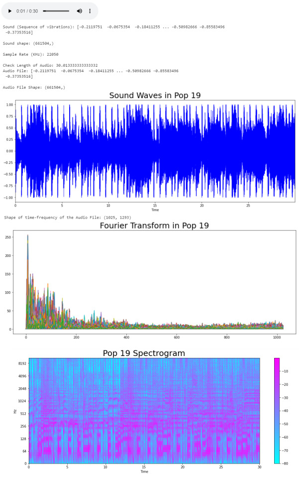
print('Sound (Sequence of vibrations):', y, '\n')

print('Sound shape:', np.shape(y), '\n')

print('Sample Rate (KHz):', sr, '\n')

# Verify length of the audio

print('Check Length of Audio:', 661794/22050)

We took the song and using the load function from the librosa library, we got an array of the audio time series (sound) and the sample rate of sound. The length of the audio is 30 seconds. Now we can trim our audio to remove the silence between songs and use the librosa.display.waveplot function to plot the audio file into a waveform. > Waveform: The waveform of an audio signal is the shape of its graph as a function of time.

# Trim silence before and after the actual audio

audio_file, _ = librosa.effects.trim(y)

print('Audio File:', audio_file, '\n')

print('Audio File Shape:', np.shape(audio_file))

#Sound Waves 2D Representation

plt.figure(figsize = (16, 6))

librosa.display.waveplot(y = audio_file, sr = sr, color = "b");

plt.title("Sound Waves in Pop 19", fontsize = 25);

After having represented the audio visually, we will plot a Fourier Transform (D) from the frequencies and amplitudes of the audio data. > Fourier Transform: A mathematical function that maps the frequency and phase content of local sections of a signal as it changes over time. This means that it takes a time-based pattern (in this case, a waveform) and retrieves the complex valued function of frequency, as a sine wave. The signal is converted into individual spectral components and provides frequency information about the signal.

#Default Fast Fourier Transforms (FFT)

n_fft = 2048 # window size

hop_length = 512 # number audio of frames between STFT columns

# Short-time Fourier transform (STFT)

D = np.abs(librosa.stft(audio_file, n_fft = n_fft, hop_length = hop_length))

print('Shape of time-frequency of the Audio File:', np.shape(D))

plt.figure(figsize = (16, 6))

plt.plot(D);

plt.title("Fourier Transform in Pop 19", fontsize = 25);

The Fourier Transform only gives us information about the frequency values and now we need a visual representation of the frequencies of the audio signal so we can calculate more audio features for our system. To do this we will plot the previous Fourier Transform (D) into a Spectrogram (DB). > Spectrogram: A visual representation of the spectrum of frequencies of a signal as it varies with time.

DB = librosa.amplitude_to_db(D, ref = np.max)

# Creating the Spectrogram

plt.figure(figsize = (16, 6))

librosa.display.specshow(DB, sr = sr, hop_length = hop_length, x_axis = 'time', y_axis = 'log'

cmap = 'cool')

plt.colorbar();

plt.title("Pop 19 Spectrogram", fontsize = 25);

The output:

Audio Features

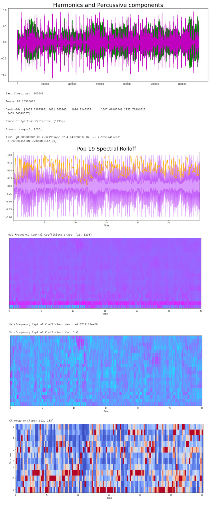
Now that we know what the audio data looks like to python, we can proceed to extract the Audio Features. The features we will need to extract, based on the provided CSV, are: · Harmonics · Percussion · Zero Crossing Rate · Tempo · Spectral Centroid · Spectral Rollof · Mel-Frequency Cepstral Coefficients · Chroma Frequencies Let’s start with the Harmonics and Percussive components:

# Decompose the Harmonics and Percussive components and show Representation

y_harm, y_perc = librosa.effects.hpss(audio_file)

plt.figure(figsize = (16, 6))

plt.plot(y_harm, color = 'g');

plt.plot(y_perc, color = 'm');

plt.title("Harmonics and Percussive components", fontsize = 25);

Using the librosa.effects.hpss function, we are able to separate the harmonics and percussive elements from the audio source and plot it into a visual representation.

Now we can retrieve the Zero Crossing Rate, using the librosa.zero_crossings function.

> Zero Crossing Rate: The rate of sign-changes (the number of times the signal changes value) of the audio signal during the frame.

#Total number of zero crossings

zero_crossings = librosa.zero_crossings(audio_file, pad=False)

print(sum(zero_crossings))

The Tempo (Beats per Minute) can be retrieved using the librosa.beat.beat_track function.

# Retrieving the Tempo in Pop 19

tempo, _ = librosa.beat.beat_track(y, sr = sr)

print('Tempo:', tempo , '\n')

The next feature extracted is the Spectral Centroids. > Spectral Centroid: a measure used in digital signal processing to characterize a spectrum. It determines the frequency area around which most of the signal energy concentrates.

# Calculate the Spectral Centroids

spectral_centroids = librosa.feature.spectral_centroid(audio_file, sr=sr)[0]

print('Centroids:', spectral_centroids, '\n')

print('Shape of Spectral Centroids:', spectral_centroids.shape, '\n')

# Computing the time variable for visualization

frames = range(len(spectral_centroids))

# Converts frame counts to time (seconds)

t = librosa.frames_to_time(frames)

print('Frames:', frames, '\n')

print('Time:', t)

Now that we have the shape of the spectral centroids as an array and the time variable (from frame counts), we need to create a function that normalizes the data. Normalization is a technique used to adjust the volume of audio files to a standard level which allows the file to be processed clearly. Once it’s normalized we proceed to retrieve the Spectral Rolloff.

> Spectral Rolloff: the frequency under which the cutoff of the total energy of the spectrum is contained, used to distinguish between sounds. The measure of the shape of the signal.

# Function that normalizes the Sound Data

def normalize(x, axis=0):

return sklearn.preprocessing.minmax_scale(x, axis=axis)

# Spectral RollOff Vector

spectral_rolloff = librosa.feature.spectral_rolloff(audio_file, sr=sr)[0]

plt.figure(figsize = (16, 6))

librosa.display.waveplot(audio_file, sr=sr, alpha=0.4, color = '#A300F9');

plt.plot(t, normalize(spectral_rolloff), color='#FFB100');

Using the audio file, we can continue to get the Mel-Frequency Cepstral Coefficients, which are a set of 20 features. In Music Information Retrieval, it’s often used to describe timbre. We will employ the librosa.feature.mfcc function.

mfccs = librosa.feature.mfcc(audio_file, sr=sr)

print('Mel-Frequency Ceptral Coefficient shape:', mfccs.shape)

#Displaying the Mel-Frequency Cepstral Coefficients:

plt.figure(figsize = (16, 6))

librosa.display.specshow(mfccs, sr=sr, x_axis='time', cmap = 'cool');

The MFCC shape is (20, 1,293), which means that the librosa.feature.mfcc function computed 20 coefficients over 1,293 frames.

mfccs = sklearn.preprocessing.scale(mfccs, axis=1)

print('Mean:', mfccs.mean(), '\n')

print('Var:', mfccs.var())

plt.figure(figsize = (16, 6))

librosa.display.specshow(mfccs, sr=sr, x_axis='time', cmap = 'cool');

Now we retrieve the Chroma Frequencies, using librosa.feature.chroma_stft. > Chroma Frequencies (or Features): are a powerful tool for analyzing music by categorizing pitches. These features capture harmonic and melodic characteristics of music.

# Increase or decrease hop_length to change how granular you want your data to be

hop_length = 5000

# Chromogram

chromagram = librosa.feature.chroma_stft(audio_file, sr=sr, hop_length=hop_length)

print('Chromogram shape:', chromagram.shape)

plt.figure(figsize=(16, 6))

librosa.display.specshow(chromagram, x_axis='time', y_axis='chroma', hop_length=hop_length, cmap='coolwarm');

The output:

Exploratory Data Analysis

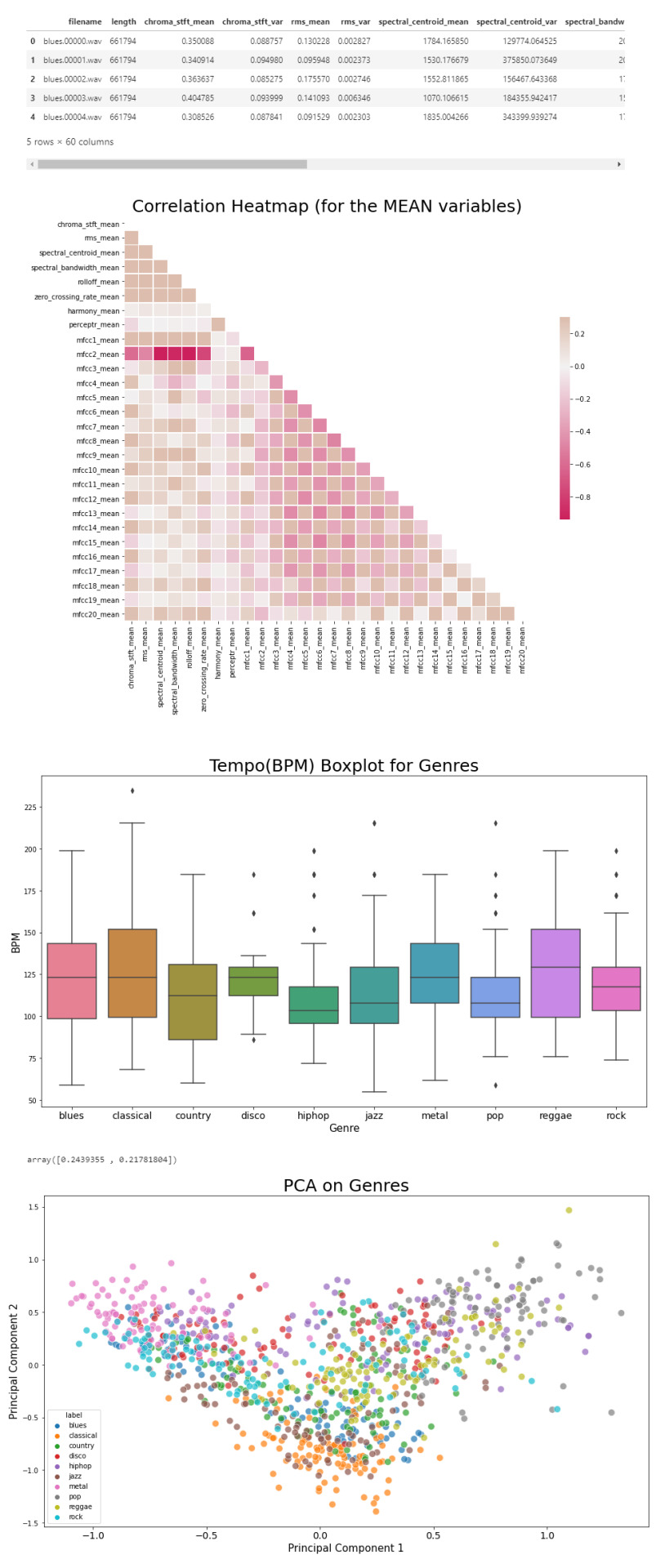
Now that we have a visual understanding of what an audio file looks like, and we’ve explored a good set of features, we can perform EDA, or Exploratory Data Analysis. This is all about getting to know the data and data profiling, summarizing the dataset through descriptive statistics. We can do this by getting a description of the data, using the describe() function or head() function. The describe() function will give us a description of all the dataset rows, and the head() function will give us the written data. We will perform EDA on the csv file, which contains all of the features previously analyzed above, and use the head() function:

# Loading the CSV file

data = pd.read_csv(f'{general_path}/features_30_sec.csv')

data.head()

Now we can create the correlation matrix of the data found in the csv file, using the feature means (average). We do this to summarize our data and pass it into a Correlation Heatmap.

# Computing the Correlation Matrix

spike_cols = [col for col in data.columns if 'mean' in col]

corr = data[spike_cols].corr()

The corr() function finds a pairwise correlation of all columns, excluding non-numeric and null values.

Now we can plot the heatmap:

# Generate a mask for the upper triangle

mask = np.triu(np.ones_like(corr, dtype=np.bool))

# Set up the matplotlib figure

f, ax = plt.subplots(figsize=(16, 11));

# Generate a custom diverging colormap

cmap = sns.diverging_palette(0, 25, as_cmap=True, s = 90, l = 45, n = 5)

# Draw the heatmap with the mask and correct aspect ratio

sns.heatmap(corr, mask=mask, cmap=cmap, vmax=.3, center=0,

square=True, linewidths=.5, cbar_kws={"shrink": .5}

plt.title('Correlation Heatmap (for the MEAN variables)', fontsize = 25)

plt.xticks(fontsize = 10)

plt.yticks(fontsize = 10);

Now we will take the data and, extracting the label(genre) and the tempo, we will draw a Box Plot. Box Plots visually show the distribution of numerical data through displaying percentiles and averages.

# Setting the axis for the box plot

x = data[["label", "tempo"]]

f, ax = plt.subplots(figsize=(16, 9));

sns.boxplot(x = "label", y = "tempo", data = x, palette = 'husl');

plt.title('Tempo(BPM) Boxplot for Genres', fontsize = 25)

plt.xticks(fontsize = 14)

plt.yticks(fontsize = 10);

plt.xlabel("Genre", fontsize = 15)

plt.ylabel("BPM", fontsize = 15)

Now we will draw a Scatter Diagram. To do this, we need to visualize possible groups of genres:

# To visualize possible groups of genres

data = data.iloc[0:, 1:]

y = data['label']

X = data.loc[:, data.columns != 'label']

We use data.iloc to get rows and columns at integer locations, and data.loc to get rows and columns with particular labels, excluding the label column. The next step is to normalize our data:

# Normalization

cols = X.columns

min_max_scaler = preprocessing.MinMaxScaler()

np_scaled = min_max_scaler.fit_transform(X)

X = pd.DataFrame(np_scaled, columns = cols)

Using the preprocessing library, we rescale each feature to a given range. Then we add a fit to data and transform (fit_transform).

We can proceed with a Principal Component Analysis:

# Principal Component Analysis

pca = PCA(n_components=2)

principalComponents = pca.fit_transform(X)

principalDf = pd.DataFrame(data = principalComponents, columns = ['principal component 1', 'principal component 2'])

# concatenate with target label

finalDf = pd.concat([principalDf, y], axis = 1)

PCA is used to reduce dimensionality in data. The fit learns some quantities from the data. Before the fit transform, the data shape was [1000, 58], meaning there’s 1000 rows with 58 columns (in the CSV file there’s 60 columns but two of these are string values, so it leaves with 58 numeric columns).

Once we use the PCA function, and set the components number to 2 we reduce the dimension of our project from 58 to 2. We have found the optimal stretch and rotation in our 58-dimension space to see the layout in two dimensions.

After reducing the dimensional space, we lose some variance(information).

pca.explained_variance_ratio_

By using this attribute we get the explained variance ratio, which we sum to get the percentage. In this case the variance explained is 46.53% .

plt.figure(figsize = (16, 9))

sns.scatterplot(x = "principal component 1", y = "principal component 2", data = finalDf, hue = "label", alpha = 0.7,

s = 100);

plt.title('PCA on Genres', fontsize = 25)

plt.xticks(fontsize = 14)

plt.yticks(fontsize = 10);

plt.xlabel("Principal Component 1", fontsize = 15)

plt.ylabel("Principal Component 2", fontsize = 15)

plt.savefig("PCA Scattert.jpg")

The output:

Genre Classification

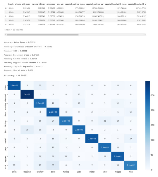
Now we know what our data looks like, the features it has and have analyzed the principal component on all genres. All we have left to do is to build a classifier model that will predict any new audio data input its genre. We will use the CSV with 10 times the data for this.

# Load the data

data = pd.read_csv(f'{general_path}/features_3_sec.csv')

data = data.iloc[0:, 1:]

data.head()

Once again visualizing and normalizing the data.

y = data['label'] # genre variable.

X = data.loc[:, data.columns != 'label'] #select all columns but not the labels

# Normalization

cols = X.columns

min_max_scaler = preprocessing.MinMaxScaler()

np_scaled = min_max_scaler.fit_transform(X)

# new data frame with the new scaled data.

X = pd.DataFrame(np_scaled, columns = cols)

Now we have to split the data for training. Like I did in my previous post, the proportions are (70:30). 70% of the data will be used for training and 30% of the data will be used for testing.

# Split the data for training

X_train, X_test, y_train, y_test = train_test_split(X, y, test_size=0.3, random_state=42)

I tested 7 algorithms but I decided to go with K Nearest-Neighbors because I had previously used it.

knn = KNeighborsClassifier(n_neighbors=19)

knn.fit(X_train, y_train)

preds = knn.predict(X_test)

print('Accuracy', ':', round(accuracy_score(y_test, preds), 5), '\n')

# Confusion Matrix

confusion_matr = confusion_matrix(y_test, preds) #normalize = 'true'

plt.figure(figsize = (16, 9))

sns.heatmap(confusion_matr, cmap="Blues", annot=True,

xticklabels = ["blues", "classical", "country", "disco", "hiphop", "jazz", "metal", "pop", "reggae", "rock"],

yticklabels=["blues", "classical", "country", "disco", "hiphop", "jazz", "metal", "pop", "reggae", "rock"]);

The output:

youtube

References

· https://medium.com/@james_52456/machine-learning-and-the-future-of-music-an-era-of-ml-artists-9be5ef27b83e

· https://www.kaggle.com/andradaolteanu/work-w-audio-data-visualise-classify-recommend/

· https://www.kaggle.com/dapy15/music-genre-classification/notebook

· https://towardsdatascience.com/how-to-start-implementing-machine-learning-to-music-4bd2edccce1f

· https://en.wikipedia.org/wiki/Music_information_retrieval

· https://pandas.pydata.org

· https://scikit-learn.org/

· https://seaborn.pydata.org

· https://matplotlib.org

· https://librosa.org/doc/main/index.html

· https://github.com/dmlc/xgboost

· https://docs.python.org/3/library/os.html

· https://www.tensorflow.org/

· https://www.hindawi.com/journals/sp/2021/1651560/

#Youtube

0 notes

chaj · 8 years ago

Link

via www.pyimagesearch.com

Continuing our series of blog posts on facial landmarks, today we are going to discuss face alignment, the process of:

Identifying the geometric structure of faces in digital images.

Attempting to obtain a canonical alignment of the face based on translation, scale, and rotation.

There are many forms of face alignment.

Some methods try to impose a (pre-defined) 3D model and then apply a transform to the input image such that the landmarks on the input face match the landmarks on the 3D model.

Other, more simplistic methods (like the one discussed in this blog post), rely only on the facial landmarks themselves (in particular, the eye regions) to obtain a normalized rotation, translation, and scale representation of the face.

The reason we perform this normalization is due to the fact that many facial recognition algorithms, including Eigenfaces, LBPs for face recognition, Fisherfaces, and deep learning/metric methods can all benefit from applying facial alignment before trying to identify the face.

Thus, face alignment can be seen as a form of “data normalization”. Just as you may normalize a set of feature vectors via zero centering or scaling to unit norm prior to training a machine learning model, it’s very common to align the faces in your dataset before training a face recognizer.

By performing this process, you’ll enjoy higher accuracy from your face recognition models.

Note: If you’re interested in learning more about creating your own custom face recognizers, be sure to refer to the PyImageSearch Gurus course where I provide detailed tutorials on face recognition.

To learn more about face alignment and normalization, just keep reading.

Looking for the source code to this post? Jump right to the downloads section.

Face alignment with OpenCV and Python

The purpose of this blog post is to demonstrate how to align a face using OpenCV, Python, and facial landmarks.

Given a set of facial landmarks (the input coordinates) our goal is to warp and transform the image to an output coordinate space.

In this output coordinate space, all faces across an entire dataset should:

Be centered in the image.

Be rotated that such the eyes lie on a horizontal line (i.e., the face is rotated such that the eyes lie along the same y-coordinates).

Be scaled such that the size of the faces are approximately identical.

To accomplish this, we’ll first implement a dedicated Python class to align faces using an affine transformation. I’ve already implemented this FaceAligner class in imutils.

Note: Affine transformations are used for rotating, scaling, translating, etc. We can pack all three of the above requirements into a single

cv2.warpAffine

call; the trick is creating the rotation matrix,

We’ll then create an example driver Python script to accept an input image, detect faces, and align them.

Finally, we’ll review the results from our face alignment with OpenCV process.

Implementing our face aligner

The face alignment algorithm itself is based on Chapter 8 of Mastering OpenCV with Practical Computer Vision Projects (Baggio, 2012), which I highly recommend if you have a C++ background or interest. The book provides open-access code samples on GitHub.

Let’s get started by examining our

FaceAligner

implementation and understanding what’s going on under the hood.

Lines 2-5 handle our imports. To read about facial landmarks and our associated helper functions, be sure to check out this previous post.

On Line 7, we begin our

FaceAligner

class with our constructor being defined on Lines 8-20.

Our constructor has 4 parameters:

predictor

: The facial landmark predictor model.

desiredLeftEye

: An optional (x, y) tuple with the default shown, specifying the desired output left eye position. For this variable, it is common to see percentages within the range of 20-40%. These percentages control how much of the face is visible after alignment. The exact percentages used will vary on an application-to-application basis. With 20% you’ll basically be getting a “zoomed in” view of the face, whereas with larger values the face will appear more “zoomed out.”

desiredFaceWidth

: Another optional parameter that defines our desired face with in pixels. We default this value to 256 pixels.

desiredFaceHeight

: The final optional parameter specifying our desired face height value in pixels.

Each of these parameters is set to a corresponding instance variable on Lines 12-15.

Next, let’s decide whether we want a square image of a face, or something rectangular. Lines 19 and 20 check if the

desiredFaceHeight

None

, and if so, we set it to the

desiredFaceWidth

, meaning that the face is square. A square image is the typical case. Alternatively, we can specify different values for both

desiredFaceWidth

and

desiredFaceHeight

to obtain a rectangular region of interest.

Now that we have constructed our

FaceAligner

object, we will next define a function which aligns the face.

This function is a bit long, so I’ve broken it up into 5 code blocks to make it more digestible:

Beginning on Line 22, we define the align function which accepts three parameters:

image

: The RGB input image.

gray

: The grayscale input image.

rect

: The bounding box rectangle produced by dlib’s HOG face detector.

On Lines 24 and 25, we apply dlib’s facial landmark predictor and convert the landmarks into (x, y)-coordinates in NumPy format.

Next, on Lines 28 and 29 we read the

left_eye

and

right_eye

regions from the

FACIAL_LANDMARK_IDXS

dictionary, found in the

helpers.py

script. These 2-tuple values are stored in left/right eye starting and ending indices.

The

leftEyePts

and

rightEyePts

are extracted from the shape list using the starting and ending indices on Lines 30 and 31.

Next, let’s will compute the center of each eye as well as the angle between the eye centroids.

This angle serves as the key component for aligning our image.

The angle of the green line between the eyes, shown in Figure 1 below, is the one that we are concerned about.

Figure 1: Computing the angle between two eyes for face alignment.

To see how the angle is computed, refer to the code block below:

On Lines 34 and 35 we compute the centroid, also known as the center of mass, of each eye by averaging all (x, y) points of each eye, respectively.

Given the eye centers, we can compute differences in (x, y)-coordinates and take the arc-tangent to obtain angle of rotation between eyes.

This angle will allow us to correct for rotation.

To determine the angle, we start by computing the delta in the y-direction,

. This is done by finding the difference between the

rightEyeCenter

and the

leftEyeCenter

on Line 38.

Similarly, we compute

, the delta in the x-direction on Line 39.

Next, on Line 40, we compute the angle of the face rotation. We use NumPy’s

arctan2

function with arguments

and

, followed by converting to degrees while subtracting 180 to obtain the angle.

In the following code block we compute the desired right eye coordinate (as a function of the left eye placement) as well as calculating the scale of the new resulting image.

# import the necessary packages from .helpers import FACIAL_LANDMARKS_IDXS from .helpers import shape_to_np import numpy as np import cv2 class FaceAligner: def __init__(self, predictor, desiredLeftEye=(0.35, 0.35), desiredFaceWidth=256, desiredFaceHeight=None): # store the facial landmark predictor, desired output left # eye position, and desired output face width + height self.predictor = predictor self.desiredLeftEye = desiredLeftEye self.desiredFaceWidth = desiredFaceWidth self.desiredFaceHeight = desiredFaceHeight # if the desired face height is None, set it to be the # desired face width (normal behavior) if self.desiredFaceHeight is None: self.desiredFaceHeight = self.desiredFaceWidth def align(self, image, gray, rect): # convert the landmark (x, y)-coordinates to a NumPy array shape = self.predictor(gray, rect) shape = shape_to_np(shape) # extract the left and right eye (x, y)-coordinates (lStart, lEnd) = FACIAL_LANDMARKS_IDXS["left_eye"] (rStart, rEnd) = FACIAL_LANDMARKS_IDXS["right_eye"] leftEyePts = shape[lStart:lEnd] rightEyePts = shape[rStart:rEnd] # compute the center of mass for each eye leftEyeCenter = leftEyePts.mean(axis=0).astype("int") rightEyeCenter = rightEyePts.mean(axis=0).astype("int") # compute the angle between the eye centroids dY = rightEyeCenter[1] - leftEyeCenter[1] dX = rightEyeCenter[0] - leftEyeCenter[0] angle = np.degrees(np.arctan2(dY, dX)) - 180 # compute the desired right eye x-coordinate based on the # desired x-coordinate of the left eye desiredRightEyeX = 1.0 - self.desiredLeftEye[0] # determine the scale of the new resulting image by taking # the ratio of the distance between eyes in the *current* # image to the ratio of distance between eyes in the # *desired* image dist = np.sqrt((dX ** 2) + (dY ** 2)) desiredDist = (desiredRightEyeX - self.desiredLeftEye[0]) desiredDist *= self.desiredFaceWidth scale = desiredDist / dist

On Line 44, we calculate the desired right eye based upon the desired left eye x-coordinate. We subtract

self.desiredLeftEye[0]

from

1.0

because the

desiredRightEyeX

value should be equidistant from the right edge of the image as the corresponding left eye x-coordinate is from its left edge.

We can then determine the

scale

of the face by taking the ratio of the distance between the eyes in the current image to the distance between eyes in the desired image

First, we compute the Euclidean distance ratio,

dist

, on Line 50.

Next, on Line 51, using the difference between the right and left eye x-values we compute the desired distance,

desiredDist

We update the

desiredDist

by multiplying it by the

desiredFaceWidth

on Line 52. This essentially scales our eye distance based on the desired width.

Finally, our scale is computed by dividing

desiredDist

by our previously calculated

dist

Now that we have our rotation

angle

and

scale

, we will need to take a few steps before we compute the affine transformation. This includes finding the midpoint between the eyes as well as calculating the rotation matrix and updating its translation component:

On Lines 57 and 58, we compute

eyesCenter

, the midpoint between the left and right eyes. This will be used in our rotation matrix calculation. In essence, this midpoint is at the top of the nose and is the point at which we will rotate the face around:

Figure 2: Computing the midpoint (blue) between two eyes. This will serve as the (x, y)-coordinate in which we rotate the face around.

To compute our rotation matrix,

, we utilize

cv2.getRotationMatrix2D

specifying

eyesCenter

angle

, and

scale

(Line 61). Each of these three values have been previously computed, so refer back to Line 40, Line 53, and Line 57 as needed.

A description of the parameters to

cv2.getRotationMatrix2D

follow:

eyesCenter

: The midpoint between the eyes is the point at which we will rotate the face around.

angle

: The angle we will rotate the face to to ensure the eyes lie along the same horizontal line.

scale

: The percentage that we will scale up or down the image, ensuring that the image scales to the desired size.

Now we must update the translation component of the matrix so that the face is still in the image after the affine transform.

On Line 64, we take half of the

desiredFaceWidth

and store the value as

, the translation in the x-direction.

To compute

, the translation in the y-direction, we multiply the

desiredFaceHeight

by the desired left eye y-value,

desiredLeftEye[1]

Using

and

, we update the translation component of the matrix by subtracting each value from their corresponding eyes midpoint value,

eyesCenter

(Lines 66 and 67).

We can now apply our affine transformation to align the face:

For convenience we store the

desiredFaceWidth

and

desiredFaceHeight

into

and

respectively (Line 70).

Then we perform our last step on Lines 70 and 71 by making a call to

cv2.warpAffine

. This function call requires 3 parameters and 1 optional parameter:

image

: The face image.

: The translation, rotation, and scaling matrix.

(w, h)

: The desired width and height of the output face.

flags

: The interpolation algorithm to use for the warp, in this case

INTER_CUBIC

. To read about the other possible flags and image transformations, please consult the OpenCV documentation.

Finally, we return the aligned face on Line 75.

Aligning faces with OpenCV and Python

Now let’s put this alignment class to work with a simple driver script. Open up a new file, name it

align_faces.py

, and let’s get to coding.

On Lines 2-7 we import required packages.

If you do not have

imutils

and/or

dlib

installed on your system, then make sure you install/upgrade them via

pip

$ pip install --upgrade imutils $ pip install --upgrad dlib

Note: If you are using Python virtual environments (as all of my OpenCV install tutorials do), make sure you use the

workon

command to access your virtual environment first, and then install/upgrade

imutils

and

dlib

Using

argparse

on Lines 10-15, we specify 2 required command line arguments:

--shape-predictor

: The dlib facial landmark predictor.

--image

: The image containing faces.

In the next block of code we initialize our HOG-based detector (Histogram of Oriented Gradients), our facial landmark predictor, and our face aligner:

Line 19 initializes our detector object using dlib’s

get_frontal_face_detector

On Line 20 we instantiate our facial landmark predictor using,

--shape-predictor

, the path to dlib’s pre-trained predictor.

We make use of the

FaceAligner

class that we just built in the previous section by initializing a an object,

, on Line 21. We specify a face width of 256 pixels.

Next, let’s load our image and prepare it for face detection:

# import the necessary packages from imutils.face_utils import FaceAligner from imutils.face_utils import rect_to_bb import argparse import imutils import dlib import cv2 # construct the argument parser and parse the arguments ap = argparse.ArgumentParser() ap.add_argument("-p", "--shape-predictor", required=True, help="path to facial landmark predictor") ap.add_argument("-i", "--image", required=True, help="path to input image") args = vars(ap.parse_args()) # initialize dlib's face detector (HOG-based) and then create # the facial landmark predictor and the face aligner detector = dlib.get_frontal_face_detector() predictor = dlib.shape_predictor(args["shape_predictor"]) fa = FaceAligner(predictor, desiredFaceWidth=256) # load the input image, resize it, and convert it to grayscale image = cv2.imread(args["image"]) image = imutils.resize(image, width=800) gray = cv2.cvtColor(image, cv2.COLOR_BGR2GRAY) # show the original input image and detect faces in the grayscale # image cv2.imshow("Input", image) rects = detector(gray, 2)

On Line 24, we load our image specified by the command line argument

–-image

. We resize the image maintaining the aspect ratio on Line 25 to have a width of 800 pixels. We then convert the image to grayscale on Line 26.

Detecting faces in the input image is handled on Line 31 where we apply dlib’s face detector. This function returns

rects

, a list of bounding boxes around the faces our detector has found.

In the next block, we iterate through

rects

, align each face, and display the original and aligned images.

We begin our loop on Line 34.

For each bounding box

rect

predicted by dlib we convert it to the format

(x, y, w, h)

(Line 37).

Subsequently, we resize the box to a width of 256 pixels, maintaining the aspect ratio, on Line 38. We store this original, but resized image, as

faceOrig

On Line 39, we align the image, specifying our image, grayscale image, and rectangle.

Finally, Lines 42 and 43 display the original and corresponding aligned face image to the screen in respective windows.

On Line 44, we wait for the user to press a key with either window in focus, before displaying the next original/aligned image pair.

The process on Lines 35-44 is repeated for all faces detected, then the script exits.

To see our face aligner in action, head to next section.

Face alignment results

Let’s go ahead and apply our face aligner to some example images. Make sure you use the “Downloads” section of this blog post to download the source code + example images.

After unpacking the archive, execute the following command:

$ python align_faces.py \ --shape-predictor shape_predictor_68_face_landmarks.dat \ --image images/example_01.jpg

From there you’ll see the following input image, a photo of myself and my financée, Trisha:

Figure 3: An input image to our OpenCV face aligner.

This image contains two faces, therefore we’ll be performing two facial alignments.

The first is seen below:

Figure 4: Aligning faces with OpenCV.

On the left we have the original detected face. The aligned face is then displayed on the right.

Now for Trisha’s face:

Figure 5: Facial alignment with OpenCV and Python.

Notice how after facial alignment both of our faces are the same scale and the eyes appear in the same output (x, y)-coordinates.

Let’s try a second example:

$ python align_faces.py \ --shape-predictor shape_predictor_68_face_landmarks.dat \ --image images/example_02.jpg

Here I am enjoying a glass of wine on Thanksgiving morning:

Figure 6: An input image to our face aligner.

After detecting my face, it is then aligned as the following figure demonstrates:

Figure 7: Using facial landmarks to align faces in images.

Here is a third example, this one of myself and my father last spring after cooking up a batch of soft shell crabs:

$ python align_faces.py \ --shape-predictor shape_predictor_68_face_landmarks.dat \ --image images/example_03.jpg

Figure 8: Another example input to our face aligner.

My father’s face is first aligned:

Figure 9: Applying facial alignment using OpenCV and Python.

Followed by my own:

Figure 10: Using face alignment to obtain canonical representations of faces.

The fourth example is a photo of my grandparents the last time they visited North Carolina:

$ python align_faces.py \ --shape-predictor shape_predictor_68_face_landmarks.dat \ --image images/example_04.jpg

Figure 11: Inputting an image to our face alignment algorithm.

My grandmother’s face is aligned first:

Figure 12: Performing face alignment using computer vision.

And then my grandfather’s:

Figure 13: Face alignment in unaffected by the person in the photo wearing glasses.

Despite both of them wearing glasses the faces are correctly aligned.

Let’s do one final example:

$ python align_faces.py \ --shape-predictor shape_predictor_68_face_landmarks.dat \ --image images/example_05.jpg

Figure 14: The final example input image to our face aligner.

After applying face detection, Trisha’s face is aligned first:

Figure 15: Facial alignment using facial landmarks.

And then my own:

Figure 16: Face alignment still works even if the input face is rotated.

The rotation angle of my face is detected and corrected, followed by being scaled to the appropriate size.

To demonstrate that this face alignment method does indeed (1) center the face, (2) rotate the face such that the eyes lie along a horizontal line, and (3) scale the faces such that they are approximately identical in size, I’ve put together a GIF animation that you can see below:

Figure 17: An animation demonstrating face alignment across multiple images.

As you can see, the eye locations and face sizes are near identical for every input image.

Summary

In today’s post, we learned how to apply facial alignment with OpenCV and Python. Facial alignment is a normalization technique, often used to improve the accuracy of face recognition algorithms, including deep learning models.

The goal of facial alignment is to transform an input coordinate space to output coordinate space, such that all faces across an entire dataset should:

Be centered in the image.

Be rotated that such the eyes lie on a horizontal line (i.e., the face is rotated such that the eyes lie along the same y-coordinates).

Be scaled such that the size of the faces are approximately identical.

All three goals can be accomplished using an affine transformation. The trick is determining the components of the transformation matrix,

Our facial alignment algorithm hinges on knowing the (x, y)-coordinates of the eyes. In this blog post we used dlib, but you can use other facial landmark libraries as well — the same techniques apply.

Facial landmarks tend to work better than Haar cascades or HOG detectors for facial alignment since we obtain a more precise estimation to eye location (rather than just a bounding box).

If you’re interested in learning more about face recognition and object detection, be sure to take a look at the PyImageSearch Gurus course where I have over 25+ lessons on these topics.

Downloads:

If you would like to download the code and images used in this post, please enter your email address in the form below. Not only will you get a .zip of the code, I’ll also send you a FREE 11-page Resource Guide on Computer Vision and Image Search Engines, including exclusive techniques that I don’t post on this blog! Sound good? If so, enter your email address and I’ll send you the code immediately!

Email address:

The post Face Alignment with OpenCV and Python appeared first on PyImageSearch.

0 notes